![]()

チュートリアル 1: 教師なし/自己教師あり学習法
第3週3日目: 教師なし学習と自己教師あり学習
Neuromatch Academy 提供
コンテンツ作成者: Arna Ghosh, Colleen Gillon, Tim Lillicrap, Blake Richards
コンテンツレビュアー: Atnafu Lambebo, Hadi Vafaei, Khalid Almubarak, Melvin Selim Atay, Kelson Shilling-Scrivo
コンテンツ編集者: Anoop Kulkarni, Spiros Chavlis
制作編集者: Deepak Raya, Gagana B, Spiros Chavlis
チュートリアルの目的
このチュートリアルでは、データの良い表現を学習することの重要性について学びます。
このチュートリアルの具体的な目的:
- 入力データに対して直接(A)およびデータから学習した表現に対して(B)ロジスティック回帰を訓練する。
- 異なるネットワークによって達成された分類性能を比較する。
- 異なるネットワークによって学習された表現を比較する。
- 教師あり学習や従来の教師なし学習法に対する自己教師あり学習の利点を特定する。
# @title Tutorial slides
from IPython.display import IFrame
link_id = "wvt34"
print(f"If you want to download the slides: https://osf.io/download/{link_id}/")
IFrame(src=f"https://mfr.ca-1.osf.io/render?url=https://osf.io/{link_id}/?direct%26mode=render%26action=download%26mode=render", width=854, height=480)
セットアップ
# @title Install dependencies

# @markdown Download dataset, modules, and files needed for the tutorial from GitHub.

# @markdown This cell will download the library from OSF, but you can check out the code in https://github.com/colleenjg/neuromatch_ssl_tutorial.git

import os, sys, shutil, importlib

REPO_PATH = "neuromatch_ssl_tutorial"
download_str = "Downloading"
if os.path.exists(REPO_PATH):
  download_str = "Redownloading"
  shutil.rmtree(REPO_PATH)

# Download from github repo directly
# !git clone git://github.com/colleenjg/neuromatch_ssl_tutorial.git --quiet

from io import BytesIO
from urllib.request import urlopen
from zipfile import ZipFile

zipurl = 'https://osf.io/smqvg/download'
print(f"{download_str} and unzipping the file... Please wait.")
with urlopen(zipurl) as zipresp:
  with ZipFile(BytesIO(zipresp.read())) as zfile:
    zfile.extractall()

# Correct now-broken use of deprecated np.product method
for module in ["data.py", "load.py", "models.py"]:
  with open(f"neuromatch_ssl_tutorial/modules/{module}", "r") as f:
    source = f.read()
    source = source.replace("np.product(", "np.prod(")
    with open(f"neuromatch_ssl_tutorial/modules/{module}", "w") as f:
      f.write(source)

print("Download completed!")
# @title Install and import feedback gadget
from vibecheck import DatatopsContentReviewContainer
def content_review(notebook_section: str):
return DatatopsContentReviewContainer(
"", # No text prompt
notebook_section,
{
"url": "https://pmyvdlilci.execute-api.us-east-1.amazonaws.com/klab",
"name": "neuromatch_dl",
"user_key": "f379rz8y",
},
).render()
feedback_prefix = "W3D3_T1"# Imports
import torch
import torchvision
import numpy as np
import matplotlib.pyplot as plt
# Import modules designed for use in this notebook.
from neuromatch_ssl_tutorial.modules import data, load, models, plot_util
from neuromatch_ssl_tutorial.modules import data, load, models, plot_util
importlib.reload(data)
importlib.reload(load)
importlib.reload(models)
importlib.reload(plot_util)# @title Figure settings
import logging
logging.getLogger('matplotlib.font_manager').disabled = True
import ipywidgets as widgets # Interactive display
%matplotlib inline
%config InlineBackend.figure_format = 'retina'
plt.style.use("https://raw.githubusercontent.com/NeuromatchAcademy/content-creation/main/nma.mplstyle")
plt.rc('axes', unicode_minus=False) # To ensure negatives render correctly with xkcd style
import warnings
warnings.filterwarnings("ignore")# @title Plotting functions
# @markdown Function to plot a histogram of RSM values: `plot_rsm_histogram(rsms, colors)`
def plot_rsm_histogram(rsms, colors, labels=None, nbins=100):
"""
Function to plot histogram based on Representational Similarity Matrices
Args:
rsms: List
List of values within RSM
colors: List
List of colors for histogram
labels: List
List of RSM Labels
nbins: Integer
Specifies number of histogram bins
Returns:
Nothing
"""
fig, ax = plt.subplots(1)
ax.set_title("Histogram of RSM values", y=1.05)
min_val = np.min([np.nanmin(rsm) for rsm in rsms])
max_val = np.max([np.nanmax(rsm) for rsm in rsms])
bins = np.linspace(min_val, max_val, nbins+1)
if labels is None:
labels = [labels] * len(rsms)
elif len(labels) != len(rsms):
raise ValueError("If providing labels, must provide as many as RSMs.")
if len(rsms) != len(colors):
raise ValueError("Must provide as many colors as RSMs.")
for r, rsm in enumerate(rsms):
ax.hist(
rsm.reshape(-1), bins, density=True, alpha=0.4,
color=colors[r], label=labels[r]
)
ax.axvline(x=0, ls="dashed", alpha=0.6, color="k")
ax.set_ylabel("Density")
ax.set_xlabel("Similarity values")
ax.legend()
plt.show()# @title Helper functions
from IPython.display import display, Image # to visualize images
# @markdown Function to set test custom torch RSM function: `test_custom_torch_RSM_fct()`
def test_custom_torch_RSM_fct(custom_torch_RSM_fct):
"""
Function to set test implementation of custom_torch_RSM_fct
Args:
custom_torch_RSM_fct: f_name
Function to test
Returns:
Nothing
"""
rand_feats = torch.rand(100, 1000)
RSM_custom = custom_torch_RSM_fct(rand_feats)
RSM_ground_truth = data.calculate_torch_RSM(rand_feats)
if torch.allclose(RSM_custom, RSM_ground_truth, equal_nan=True):
print("custom_torch_RSM_fct() is correctly implemented.")
else:
print("custom_torch_RSM_fct() is NOT correctly implemented.")
# @markdown Function to set test custom contrastive loss function: `test_custom_contrastive_loss_fct()`
def test_custom_contrastive_loss_fct(custom_simclr_contrastive_loss):
"""
Function to set test implementation of custom_simclr_contrastive_loss
Args:
custom_simclr_contrastive_loss: f_name
Function to test
Returns:
Nothing
"""
rand_proj_feat1 = torch.rand(100, 1000)
rand_proj_feat2 = torch.rand(100, 1000)
loss_custom = custom_simclr_contrastive_loss(rand_proj_feat1, rand_proj_feat2)
loss_ground_truth = models.contrastive_loss(rand_proj_feat1,rand_proj_feat2)
if torch.allclose(loss_custom, loss_ground_truth):
print("custom_simclr_contrastive_loss() is correctly implemented.")
else:
print("custom_simclr_contrastive_loss() is NOT correctly implemented.")# @title Set random seed
# @markdown Executing `set_seed(seed=seed)` you are setting the seed
# For DL its critical to set the random seed so that students can have a
# baseline to compare their results to expected results.
# Read more here: https://pytorch.org/docs/stable/notes/randomness.html
# Call `set_seed` function in the exercises to ensure reproducibility.
import random
import torch
def set_seed(seed=None, seed_torch=True):
"""
Handles variability by controlling sources of randomness
through set seed values
Args:
seed: Integer
Set the seed value to given integer.
If no seed, set seed value to random integer in the range 2^32
seed_torch: Bool
Seeds the random number generator for all devices to
offer some guarantees on reproducibility
Returns:
Nothing
"""
if seed is None:
seed = np.random.choice(2 ** 32)
random.seed(seed)
np.random.seed(seed)
if seed_torch:
torch.manual_seed(seed)
torch.cuda.manual_seed_all(seed)
torch.cuda.manual_seed(seed)
torch.backends.cudnn.benchmark = False
torch.backends.cudnn.deterministic = True
print(f'Random seed {seed} has been set.')
# In case that `DataLoader` is used
def seed_worker(worker_id):
"""
DataLoader will reseed workers following randomness in
multi-process data loading algorithm.
Args:
worker_id: integer
ID of subprocess to seed. 0 means that
the data will be loaded in the main process
Refer: https://pytorch.org/docs/stable/data.html#data-loading-randomness for more details
Returns:
Nothing
"""
worker_seed = torch.initial_seed() % 2**32
np.random.seed(worker_seed)
random.seed(worker_seed)# @title Set device (GPU or CPU). Execute `set_device()`
# especially if torch modules used.
# Inform the user if the notebook uses GPU or CPU.
def set_device():
"""
Set the device. CUDA if available, CPU otherwise
Args:
None
Returns:
Nothing
"""
device = "cuda" if torch.cuda.is_available() else "cpu"
if device != "cuda":
print("WARNING: For this notebook to perform best, "
"if possible, in the menu under `Runtime` -> "
"`Change runtime type.` select `GPU` ")
else:
print("GPU is enabled in this notebook.")
return device# Set global variables
SEED = 2021
set_seed(seed=SEED)
DEVICE = set_device()# @markdown ### Pre-load variables (allows each section to be run independently)
# Section 1
dSprites = data.dSpritesDataset(
os.path.join(REPO_PATH, "dsprites", "dsprites_subset.npz")
)
dSprites_torchdataset = data.dSpritesTorchDataset(
dSprites,
target_latent="shape"
)
train_sampler, test_sampler = data.train_test_split_idx(
dSprites_torchdataset,
fraction_train=0.8,
randst=SEED
)
supervised_encoder = load.load_encoder(REPO_PATH,
model_type="supervised",
verbose=False)
# Section 2
custom_torch_RSM_fct = None # Default is used instead
# Section 3
random_encoder = load.load_encoder(REPO_PATH,
model_type="random",
verbose=False)
# Section 4
vae_encoder = load.load_encoder(REPO_PATH,
model_type="vae",
verbose=False)
# Section 5
invariance_transforms = torchvision.transforms.RandomAffine(
degrees=90,
translate=(0.2, 0.2),
scale=(0.8, 1.2)
)
dSprites_invariance_torchdataset = data.dSpritesTorchDataset(
dSprites,
target_latent="shape",
simclr=True,
simclr_transforms=invariance_transforms
)
# Section 6
simclr_encoder = load.load_encoder(REPO_PATH,
model_type="simclr",
verbose=False)セクション0: はじめに
# @title Video 0: Introduction
from ipywidgets import widgets
from IPython.display import YouTubeVideo
from IPython.display import IFrame
from IPython.display import display


class PlayVideo(IFrame):
  def __init__(self, id, source, page=1, width=400, height=300, **kwargs):
    self.id = id
    if source == 'Bilibili':
      src = f'https://player.bilibili.com/player.html?bvid={id}&page={page}'
    elif source == 'Osf':
      src = f'https://mfr.ca-1.osf.io/render?url=https://osf.io/download/{id}/?direct%26mode=render'
    super(PlayVideo, self).__init__(src, width, height, **kwargs)


def display_videos(video_ids, W=400, H=300, fs=1):
  tab_contents = []
  for i, video_id in enumerate(video_ids):
    out = widgets.Output()
    with out:
      if video_ids[i][0] == 'Youtube':
        video = YouTubeVideo(id=video_ids[i][1], width=W,
                             height=H, fs=fs, rel=0)
        print(f'Video available at https://youtube.com/watch?v={video.id}')
      else:
        video = PlayVideo(id=video_ids[i][1], source=video_ids[i][0], width=W,
                          height=H, fs=fs, autoplay=False)
        if video_ids[i][0] == 'Bilibili':
          print(f'Video available at https://www.bilibili.com/video/{video.id}')
        elif video_ids[i][0] == 'Osf':
          print(f'Video available at https://osf.io/{video.id}')
      display(video)
    tab_contents.append(out)
  return tab_contents


video_ids = [('Youtube', 'Q3b_EqFUI00'), ('Bilibili', 'BV1D64y1s78e')]
tab_contents = display_videos(video_ids, W=854, H=480)
tabs = widgets.Tab()
tabs.children = tab_contents
for i in range(len(tab_contents)):
  tabs.set_title(i, video_ids[i][0])
display(tabs)
# @title Submit your feedback
content_review(f"{feedback_prefix}_Introduction_Video")セクション1: 表現は重要である
所要時間の目安: 約30分
# @title Video 1: Why do representations matter?
from ipywidgets import widgets
from IPython.display import YouTubeVideo
from IPython.display import IFrame
from IPython.display import display


class PlayVideo(IFrame):
  def __init__(self, id, source, page=1, width=400, height=300, **kwargs):
    self.id = id
    if source == 'Bilibili':
      src = f'https://player.bilibili.com/player.html?bvid={id}&page={page}'
    elif source == 'Osf':
      src = f'https://mfr.ca-1.osf.io/render?url=https://osf.io/download/{id}/?direct%26mode=render'
    super(PlayVideo, self).__init__(src, width, height, **kwargs)


def display_videos(video_ids, W=400, H=300, fs=1):
  tab_contents = []
  for i, video_id in enumerate(video_ids):
    out = widgets.Output()
    with out:
      if video_ids[i][0] == 'Youtube':
        video = YouTubeVideo(id=video_ids[i][1], width=W,
                             height=H, fs=fs, rel=0)
        print(f'Video available at https://youtube.com/watch?v={video.id}')
      else:
        video = PlayVideo(id=video_ids[i][1], source=video_ids[i][0], width=W,
                          height=H, fs=fs, autoplay=False)
        if video_ids[i][0] == 'Bilibili':
          print(f'Video available at https://www.bilibili.com/video/{video.id}')
        elif video_ids[i][0] == 'Osf':
          print(f'Video available at https://osf.io/{video.id}')
      display(video)
    tab_contents.append(out)
  return tab_contents


video_ids = [('Youtube', 'lj5uTUo6W88'), ('Bilibili', 'BV1g54y1J7cE')]
tab_contents = display_videos(video_ids, W=854, H=480)
tabs = widgets.Tab()
tabs.children = tab_contents
for i in range(len(tab_contents)):
  tabs.set_title(i, video_ids[i][0])
display(tabs)
# @title Submit your feedback
content_review(f"{feedback_prefix}_Why_do_representations_matter_Video")セクション1.1: dSpritesデータセットの紹介
このチュートリアルでは、公開されているdSpritesデータセットのサブセットを使用して、良い表現を学習することの重要性を調査します。
データセットについての注意: 便宜上、GitHubのこちらで公開されている元の完全なデータセットのサブセットを使用します。
インタラクティブデモ1.1.1: dSpritesデータセットの探索
最初のデモでは、dSpritesデータセットについて理解を深めます。このデータセットは白黒画像で構成されており(使用するサブセットでは合計20,000枚の画像があります)。
データセット内の画像は、以下の潜在変数の値の組み合わせで表現できます:
- 形状 (3種類): 正方形 (1.0)、楕円 (2.0)、ハート (3.0)
- スケール (6段階): 0.5から1.0まで
- 向き (40段階): 0から2まで
- X位置 (32段階): 0から1まで(左から右)
- Y位置 (32段階): 0から1まで(上から下)
結果として、各画像には5つのラベルが付与されています。 潜在変数のそれぞれに対応しています。
まず、data.dSpritesDatasetクラスのインスタンスであるdSpritesオブジェクトにデータセットを読み込みます。
dSprites = data.dSpritesDataset(
    os.path.join(REPO_PATH, "dsprites", "dsprites_subset.npz")
)次に、dSpritesDatasetクラスのメソッドを使って、データセットからいくつかの画像をプロットし、それぞれの潜在変数の値を画像の下に表示します。
インタラクティブデモ: ランダム状態引数randstに任意の整数またはNoneを渡すことで、異なるランダムサンプリングされた画像セットを表示できます。(元の設定はrandst=SEEDです。)
# DEMO: To view different images, set randst to any integer value.
dSprites.show_images(num_images=10, randst=SEED)posXとposYの潜在変数(ボーナス2で最も関連するもの)をよりよく理解するために、注釈付きの画像をプロットします。注釈(赤色)は実際の画像を変更するものではなく、視覚化のためだけに追加されており、以下を示しています:
posXとposYの範囲の端- 各形状の中心点、すなわち
(posX, posY)
形状の位置についての注意: すべての形状の中心は赤い四角で示された領域内に位置しています。posXとposYはこの領域内での形状の中心の相対位置を示しており、posX=0(左端)からposX=1(右端)、posY=0(上端)からposY=1(下端)までです。バッファ領域の外に形状の中心は現れません。このdSpritesデータセットの設計により、異なるスケールや回転の形状がすべて完全に表示されることが保証されています。
# DEMO: To view different images, set randst to any integer value.
dSprites.show_images(num_images=10, randst=SEED, annotations="pos")
セクション1.2: 表現の有無による分類器の訓練
ここでは、dSpritesデータセットの画像の形状潜在変数をデコードするために訓練された2種類の分類器の性能を調査します。
具体的には、1つは画像に直接訓練された分類器、もう1つはエンコーダーネットワークの出力に対して訓練された分類器です。
ここでおよびチュートリアル全体で使用するエンコーダーネットワークは、以下の図に示す多層畳み込みネットワークです。2つの連続した畳み込み層の後に3つの全結合層が続き、層間には平均プーリングとバッチ正規化が使われ、非線形活性化関数としてReLUが用いられています。
分類器層はエンコーダーの特徴量を入力として受け取り、例えばエンコードされた入力画像の形状潜在変数を予測します。
用語についての注意: このチュートリアルでは、表現と特徴量の両方の用語が、エンコーダーネットワークの最終層で学習されるデータ埋め込み(1x84の次元で、赤い破線の枠で示されている)を指し、これが分類器に入力されます。
# @markdown ### Encoder network schematic
Image(filename=os.path.join(REPO_PATH, "images", "feat_encoder_schematic.png"), width=1200)
以下のコードは:
- 関数を使ってランダム処理を行うモジュールにシードを設定し、結果の再現性を確保し、
data.dSpritesTorchDatasetクラスを使ってdSpritesデータセットをtorchデータセットにまとめ、- 関数を使って訓練用とテスト用のサンプラーを初期化し、2つのデータセットを分けています。
# Set the seed before building any dataset/network initializing or training,
# to ensure reproducibility
set_seed(SEED)

# Initialize a torch dataset, specifying the target latent dimension for
# the classifier
dSprites_torchdataset = data.dSpritesTorchDataset(
  dSprites,
  target_latent="shape"
  )

# Initialize a train_sampler and a test_sampler to keep the two sets
# consistently separate
train_sampler, test_sampler = data.train_test_split_idx(
  dSprites_torchdataset,
  fraction_train=0.8,  # 80:20 data split
  randst=SEED
  )

print(f"Dataset size: {len(train_sampler)} training, "
      f"{len(test_sampler)} test images")
インタラクティブデモ1.2.1: 画像に直接ロジスティック回帰分類器を訓練する
以下のコードは:
- 訓練セットの画像に直接ロジスティック回帰を訓練し、形状を分類し、関数を使ってテストセットの画像で性能を評価します。
インタラクティブデモ: num_epochsの値を1から50の間で変えて、訓練回数が増えると性能が向上するか試してみてください。(元の設定はnum_epochs=25です。)
# @title Submit your feedback
content_review(f"{feedback_prefix}_What_models_Video")
# Call this before any dataset/network initializing or training,
# to ensure reproducibility
set_seed(SEED)
num_epochs = 25 # DEMO: Try different numbers of training epochs
# Train a classifier directly on the images
print("Training a classifier directly on the images...")
_ = models.train_classifier(
encoder=None,
dataset=dSprites_torchdataset,
train_sampler=train_sampler,
test_sampler=test_sampler,
freeze_features=True, # There is no feature encoder to train here, anyway
num_epochs=num_epochs,
verbose=True # Print results
)観察すると、画像に直接訓練された分類器は、25エポックの訓練後、テストセットでわずかにチャンスを上回る性能(39.55%)を示しています。
異なる特徴エンコーダーを用いた形状分類結果:
| チャンス | なし(生データ) | |
|---|---|---|
| 33.33% | 39.55% |
コーディング演習1.2.1: エンコーダーと共にロジスティック回帰分類器を訓練する
以下のコードは:
- 上で初期化した同じdSprites torchデータセット(
dSprites_torchdataset)と訓練・テストサンプラー(train_sampler,test_sampler)を使用し、 - 再現性を確保するためにランダム処理を行うサブ構造にシードを設定し、
- 教師ありネットワークで使用するエンコーダーネットワークを
models.EncoderCoreクラスで初期化し、 - 分類器とエンコーダーの訓練に使うエポック数の提案値を設定します(
num_epochs=10)。
演習: を使って、エンコーダーと共に分類器を訓練し、入力画像の形状を分類してください。性能はどうなりますか?
ヒント:
- :
- インタラクティブデモ1.2.1で紹介されています。
freeze_featuresという引数を取ります:Trueに設定するとエンコーダーは固定され、分類器層のみが訓練されます。Falseに設定するとエンコーダーは固定されず、分類器層と共に訓練されます。
def train_supervised_encoder(num_epochs, seed):
  """
  Helper function to train the encoder in a supervised way

  Args:
    num_epochs: Integer
      Number of epochs the supervised encoder is to be trained for
    seed: Integer
      The seed value for the dataset/network

  Returns:
    supervised_encoder: nn.module
      The trained encoder with mentioned parameters/hyperparameters
  """
  # Call this before any dataset/network initializing or training,
  # to ensure reproducibility
  set_seed(seed)

  # Initialize a core encoder network on which the classifier will be added
  supervised_encoder = models.EncoderCore()

  #################################################
  # Fill in missing code below (...),
  # then remove or comment the line below to test your implementation
  raise NotImplementedError("Exercise: Train a supervised encoder and classifier.")
  #################################################
  # Train an encoder and classifier on the images, using models.train_classifier()
  print("Training a supervised encoder and classifier...")
  _ = models.train_classifier(
      encoder=...,
      dataset=...,
      train_sampler=...,
      test_sampler=...,
      freeze_features=...,
      num_epochs=num_epochs,
      verbose=...  # print results
      )

  return supervised_encoder


num_epochs = 10  # Proposed number of training epochs
## Uncomment below to test your function
# supervised_encoder = train_supervised_encoder(num_epochs=num_epochs, seed=SEED)
エンコーダーと分類器の訓練10エポック後のネットワーク性能(チャンス: 33.33%):
訓練精度: 100.00%
テスト精度: 98.70%
# @title Submit your feedback
content_review(f"{feedback_prefix}_Logistic_regression_classifier_Exercise")
しかし、エンコーダーネットワークと共に訓練された分類器は、わずか10エポックの訓練後にテストセットで非常に高い分類精度(約98.70%)を達成します。
異なる特徴エンコーダーを用いた形状分類結果:
| チャンス | なし(生データ) | 教師あり | |
|---|---|---|---|
| 33.33% | 39.55% | 98.70% |
セクション2: 教師あり学習は不変な表現を誘導する
所要時間の目安: 約20分
# @title Video 2: Supervised Learning and Invariance
from ipywidgets import widgets
from IPython.display import YouTubeVideo
from IPython.display import IFrame
from IPython.display import display


class PlayVideo(IFrame):
  def __init__(self, id, source, page=1, width=400, height=300, **kwargs):
    self.id = id
    if source == 'Bilibili':
      src = f'https://player.bilibili.com/player.html?bvid={id}&page={page}'
    elif source == 'Osf':
      src = f'https://mfr.ca-1.osf.io/render?url=https://osf.io/download/{id}/?direct%26mode=render'
    super(PlayVideo, self).__init__(src, width, height, **kwargs)


def display_videos(video_ids, W=400, H=300, fs=1):
  tab_contents = []
  for i, video_id in enumerate(video_ids):
    out = widgets.Output()
    with out:
      if video_ids[i][0] == 'Youtube':
        video = YouTubeVideo(id=video_ids[i][1], width=W,
                             height=H, fs=fs, rel=0)
        print(f'Video available at https://youtube.com/watch?v={video.id}')
      else:
        video = PlayVideo(id=video_ids[i][1], source=video_ids[i][0], width=W,
                          height=H, fs=fs, autoplay=False)
        if video_ids[i][0] == 'Bilibili':
          print(f'Video available at https://www.bilibili.com/video/{video.id}')
        elif video_ids[i][0] == 'Osf':
          print(f'Video available at https://osf.io/{video.id}')
      display(video)
    tab_contents.append(out)
  return tab_contents


video_ids = [('Youtube', 'ZQka4k8ZOs0'), ('Bilibili', 'BV1d54y1E76W')]
tab_contents = display_videos(video_ids, W=854, H=480)
tabs = widgets.Tab()
tabs.children = tab_contents
for i in range(len(tab_contents)):
  tabs.set_title(i, video_ids[i][0])
display(tabs)
# @title Submit your feedback
content_review(f"{feedback_prefix}_Supervised_learning_and_invariance_Video")セクション2.1: 表現類似性行列(RSM)の検証
エンコーダーネットワークが学習した表現を調べるために、**表現類似性行列(RSM)**を使用します。これらの行列では、エンコーダーの表現が各画像ペア間でどれだけ類似しているかをプロットし、表現空間の全体構造を明らかにします。
コサイン類似度についての注意: ここでは表現の類似度の尺度としてコサイン類似度を用いています。コサイン類似度は2つのベクトル間の角度を測定し、正規化された内積と考えることができます。
コーディング演習2.1.1: RSMを計算する関数を完成させる
以下のコードは:
- 特徴量からRSMを計算する関数の骨組みを示し、
- カスタム関数を解答実装と比較してテストします。
演習: の実装を完成させてください。
ヒント:
- :
- 1つの入力引数を取ります:
features(2次元torchテンソル): 特徴行列(項目数×特徴数)
- 1つの出力を返します:
rsm(2次元torchテンソル): 類似度行列(項目数×項目数)
- を使用します。
- 1つの入力引数を取ります:
- :
- 順に3つの引数を取ります:
x1(torchテンソル),x2(torchテンソル),dim(整数)
x1とx2の間の類似度をdim次元に沿って返します。
- 順に3つの引数を取ります:
詳細なヒント:
- を使って、
featuresのすべての可能なペアの項目間の類似度を測るには:featuresの2つのバージョンをそれぞれx1とx2に渡します。x1とx2で特徴量の次元が同じ位置にあることを確認し、その次元をdimで指定します。- すべてのペアの類似度を得るために、
x1とx2で**項目の次元が直交(異なる位置)**していることを確認します。 - これを実現するために、長さ1の次元(シングルトン次元)を使うことを忘れないでください。
def custom_torch_RSM_fct(features):
  """
  Custom function to calculate representational similarity matrix (RSM) of a feature
  matrix using pairwise cosine similarity.

  Args:
    features: 2D torch.Tensor
      Feature matrix of size (nbr items x nbr features)

  Returns:
    rsm: 2D torch.Tensor
      Similarity matrix of size (nbr items x nbr items)
  """

  num_items, num_features = features.shape

  #################################################
  # Fill in missing code below (...),
  # Complete the function below given the specific guidelines.
  # Use torch.nn.functional.cosine_similarity()
  # then remove or comment the line below to test your function
  raise NotImplementedError("Exercise: Implement RSM calculation.")
  #################################################
  # EXERCISE: Implement RSM calculation
  rsm = ...

  if not rsm.shape == (num_items, num_items):
    raise ValueError(f"RSM should be of shape ({num_items}, {num_items})")

  return rsm


## Test implementation by comparing output to solution implementation
# test_custom_torch_RSM_fct(custom_torch_RSM_fct)
custom_torch_RSM_fct()は正しく実装されています。
# @title Submit your feedback
content_review(f"{feedback_prefix}_Function_that_calculates_RSMs_Exercise")
インタラクティブデモ 2.1.1: 監督型ネットワークエンコーダの潜在次元ごとのRSMのプロット
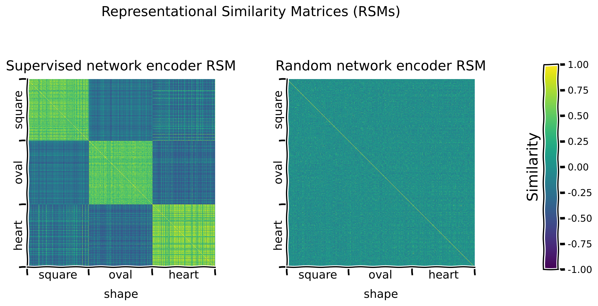
このデモでは、監督型ネットワークエンコーダによって生成されたテストセット画像の表現に対するRSMを計算します。
以下のコードは:
- を使って、指定された潜在次元(例:
sorting_latent="shape")に基づいて行と列をソートしたテストセットのRSMを計算し、プロットします。
インタラクティブデモ: 現在の例では、RSMの行と列は shape 潜在次元に沿って整理されています。他の潜在次元("scale"、"orientation"、"posX"、または "posY")に沿って整理してみて、異なるパターンが現れるかどうかを確認してください。(元の設定は sorting_latent="shape" です。)
sorting_latent = "shape"  # DEMO: Try sorting by different latent dimensions
print("Plotting RSMs...")
_ = models.plot_model_RSMs(
    encoders=[supervised_encoder],  # We pass the trained supervised_encoder
    dataset=dSprites_torchdataset,
    sampler=test_sampler,  # We want to see the representations on the held out test set
    titles=["Supervised network encoder RSM"],  # Plot title
    sorting_latent=sorting_latent,
    )
# @title Submit your feedback
content_review(f"{feedback_prefix}_Supervised_network_encoder_RSM_Interactive_Demo")議論 2.1.1: エンコーダが異なる画像をどのように表現しているか、RSMはどのようなパターンを示していますか?
A. 左上から右下に伸びる黄色(最大類似度色)の対角線は何を表していますか?
B. 類似した潜在値を共有する画像のペア(例:2つのハート画像)と、そうでない画像のペア(例:ハートと四角形の画像)を比較したとき、どのようなパターンが観察されますか?
C. いくつかの形状は他よりも類似してエンコードされているように見えますか?
D. いくつかの潜在次元は他よりも明確なRSMパターンを示していますか?それはなぜでしょうか?
# @markdown #### Supporting images for Discussion response examples for 2.1.1
Image(filename=os.path.join(REPO_PATH, "images", "rsms_supervised_encoder_10ep_bs1000_seed2021.png"), width=1200)# @title Submit your feedback
content_review(f"{feedback_prefix}_What_patterns_do_the_RSMs_reveal_Discussion")セクション 3: ランダム射影はあまりうまく機能しない
所要時間の目安:約20分
# @title Video 3: Random Representations
from ipywidgets import widgets
from IPython.display import YouTubeVideo
from IPython.display import IFrame
from IPython.display import display


class PlayVideo(IFrame):
  def __init__(self, id, source, page=1, width=400, height=300, **kwargs):
    self.id = id
    if source == 'Bilibili':
      src = f'https://player.bilibili.com/player.html?bvid={id}&page={page}'
    elif source == 'Osf':
      src = f'https://mfr.ca-1.osf.io/render?url=https://osf.io/download/{id}/?direct%26mode=render'
    super(PlayVideo, self).__init__(src, width, height, **kwargs)


def display_videos(video_ids, W=400, H=300, fs=1):
  tab_contents = []
  for i, video_id in enumerate(video_ids):
    out = widgets.Output()
    with out:
      if video_ids[i][0] == 'Youtube':
        video = YouTubeVideo(id=video_ids[i][1], width=W,
                             height=H, fs=fs, rel=0)
        print(f'Video available at https://youtube.com/watch?v={video.id}')
      else:
        video = PlayVideo(id=video_ids[i][1], source=video_ids[i][0], width=W,
                          height=H, fs=fs, autoplay=False)
        if video_ids[i][0] == 'Bilibili':
          print(f'Video available at https://www.bilibili.com/video/{video.id}')
        elif video_ids[i][0] == 'Osf':
          print(f'Video available at https://osf.io/{video.id}')
      display(video)
    tab_contents.append(out)
  return tab_contents


video_ids = [('Youtube', 'LVM7Fm5T6Fs'), ('Bilibili', 'BV1Jf4y15789')]
tab_contents = display_videos(video_ids, W=854, H=480)
tabs = widgets.Tab()
tabs.children = tab_contents
for i in range(len(tab_contents)):
  tabs.set_title(i, video_ids[i][0])
display(tabs)
# @title Submit your feedback
content_review(f"{feedback_prefix}_Random_representations_Video")セクション 3.1: ランダムエンコーダのRSMを調べる
教師ありネットワークエンコーダのRSMで観察されるパターンが自明なものかどうかを判断するために、未学習エンコーダのランダム射影からも同様のパターンが現れるかを調査します。
コーディング演習 3.1.1: 異なる潜在次元に沿ったランダムネットワークエンコーダのRSMをプロットする
この演習では、セクション 2.1 と同じ解析をランダムエンコーダで繰り返します。
以下のコードは:
models.EncoderCoreクラスを使ってランダムネットワーク用のエンコーダネットワークを初期化し、- 行と列をソートする潜在次元(
sorting_latent="shape")を提案します。
演習:
- 教師ありネットワークエンコーダとランダムネットワークエンコーダのRSMを、 を使って可視化してください。
- 異なる潜在次元(
"scale"、"orientation"、"posX"、または"posY")に沿って整理されたRSMを可視化し、教師ありエンコーダネットワークとランダムエンコーダネットワークで観察されるパターンを比較してください。
ヒント: は インタラクティブデモ 2.1.1 で紹介されています。
def plot_rsms(seed):
  """
  Helper function to plot Representational Similarity Matrices (RSMs)

  Args:
    seed: Integer
      The seed value for the dataset/network

  Returns:
    random_encoder: nn.module
      The encoder with mentioned parameters/hyperparameters
  """
  # Call this before any dataset/network initializing or training,
  # to ensure reproducibility
  set_seed(seed)

  # Initialize a core encoder network that will not get trained
  random_encoder = models.EncoderCore()

  # Try sorting by different latent dimensions
  sorting_latent = "shape"

  #################################################
  # Fill in missing code below (...),
  # then remove or comment the line below to test your implementation
  raise NotImplementedError("Exercise: Plot RSMs.")
  #################################################
  # Plot RSMs
  print("Plotting RSMs...")
  _ = models.plot_model_RSMs(
      encoders=[..., ...],  # Pass both encoders
      dataset=...,
      sampler=...,  # To see the representations on the held out test set
      titles=["Supervised network encoder RSM",
              "Random network encoder RSM"],  # Plot titles
      sorting_latent=sorting_latent,
      )

  return random_encoder


## Uncomment below to test your function
# random_encoder = plot_rsms(seed=SEED)出力例:
# @title Submit your feedback
content_review(f"{feedback_prefix}_Plotting_a_random_network_encoder_Exercise")
ディスカッション 3.1.1: これらのRSMを比較することで、訓練済みエンコーダ表現とランダムエンコーダ表現の潜在的価値について何が明らかになるか?
A. ランダムネットワークエンコーダのRSMには、どのようなパターンが見られるか?
B. どのエンコーダネットワークが意味のある表現を生成する可能性が最も高いか?
# @markdown #### Supporting images for Discussion response examples for 3.1.1: All random encoder RSMs
Image(filename=os.path.join(REPO_PATH, "images", "rsms_random_encoder_0ep_bs0_seed2021.png"), width=1000)# @title Submit your feedback
content_review(f"{feedback_prefix}_Trained_vs_Random_encoder_Discussion")コーディング演習 3.1.2: ランダムネットワークエンコーダによって生成された表現を用いたロジスティック回帰の分類性能評価
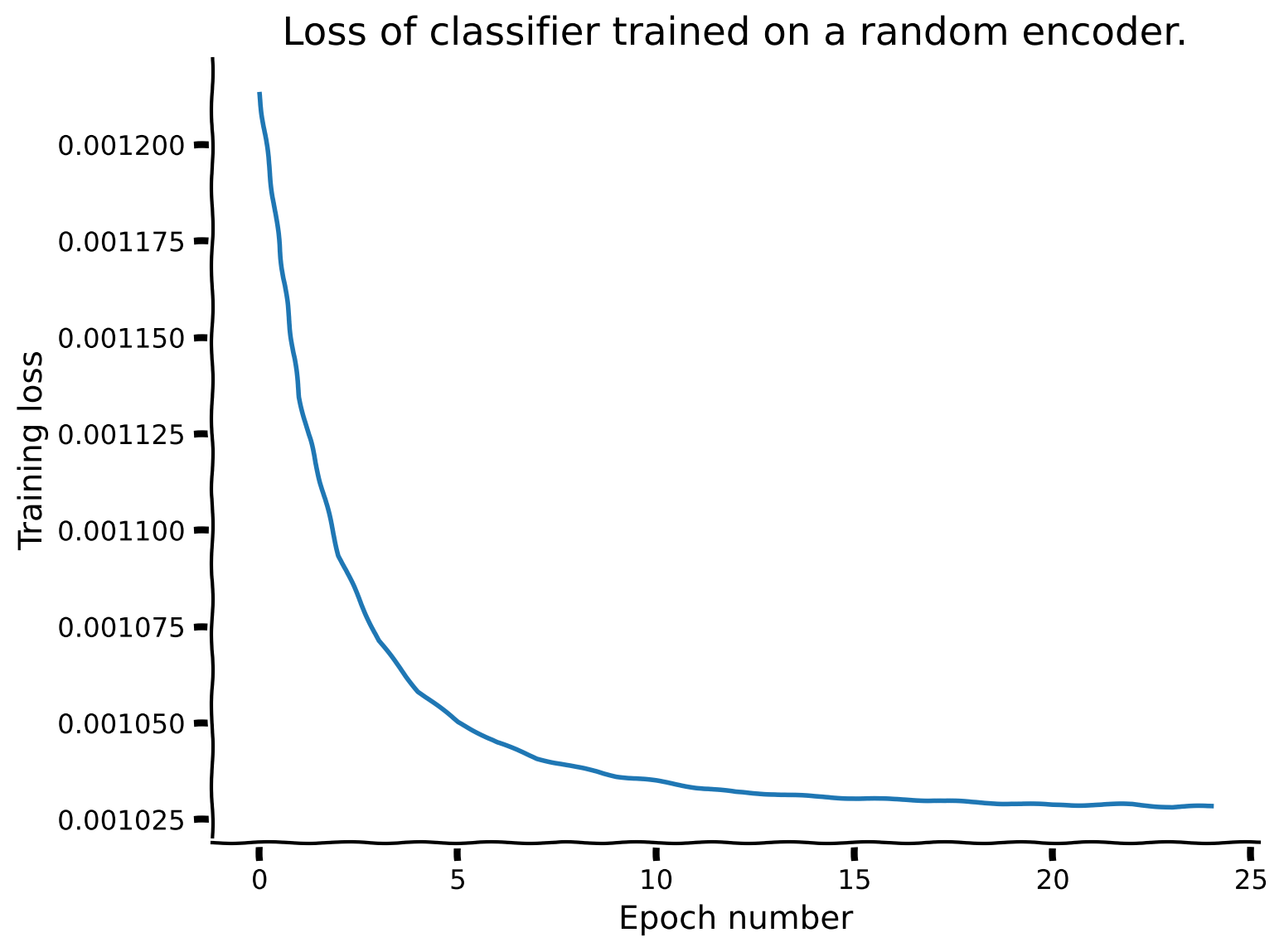
この演習では、セクション1.2と同様の分析をランダムエンコーダネットワークで繰り返します。重要なのは、今回はエンコーダのパラメータを凍結し (freeze_features=True を設定)、訓練中に更新しないことです。事前に適切な訓練エポック数の提案を与えられる代わりに、訓練損失の配列を用いて適切な値を選択します。
以下のコードは:
- ランダムエンコーダネットワークの上にロジスティック回帰を訓練し、形状に基づいて画像を分類します。
- を用いてテストセット画像での性能を評価します。この際、
freeze_features=Trueによりエンコーダは訓練されず、分類器のみが訓練されることを保証します。
演習:
- 分類器を訓練するエポック数を設定してください。
- モデル訓練時に返される訓練損失配列 (
random_loss_array、すなわち各エポックでの訓練損失) をプロットしてください。 - 訓練損失の推移に基づき、必要ならば分類器の訓練エポック数を増やして再実行してください。
def plot_loss(num_epochs, seed):
  """
  Helper function to plot the loss function of the random-encoder

  Args:
    num_epochs: Integer
      Number of the epochs the random encoder is to be trained for
    seed: Integer
      The seed value for the dataset/network

  Returns:
    random_loss_array: List
      Loss per epoch
  """
  # Call this before any dataset/network initializing or training,
  # to ensure reproducibility
  set_seed(seed)

  # Train classifier on the randomly encoded images
  print("Training a classifier on the random encoder representations...")
  _, random_loss_array, _, _ = models.train_classifier(
      encoder=random_encoder,
      dataset=dSprites_torchdataset,
      train_sampler=train_sampler,
      test_sampler=test_sampler,
      freeze_features=True,  # Keep the encoder frozen while training the classifier
      num_epochs=num_epochs,
      verbose=True  # Print results
      )
  #################################################
  # Fill in missing code below (...),
  # then remove or comment the line below to test your implementation
  raise NotImplementedError("Exercise: Plot loss array.")
  #################################################
  # Plot the loss array
  fig, ax = plt.subplots()
  ax.plot(...)
  ax.set_title(...)
  ax.set_xlabel(...)
  ax.set_ylabel(...)

  return random_loss_array


## Set a reasonable number of training epochs
num_epochs = 25
## Uncomment below to test your plot
# random_loss_array = plot_loss(num_epochs=num_epochs, seed=SEED)
分類器訓練25エポック後のネットワーク性能(偶然の確率: 33.33%):
訓練精度: 46.02%
テスト精度: 44.67%
出力例:
# @title Submit your feedback
content_review(f"{feedback_prefix}_Evaluating_the_classification_performance_Exercise")
ネットワークの損失は25エポック時点で比較的安定しており、その時点で分類器はテストデータセットに対して44.67%の精度を示しています。
異なる特徴エンコーダを用いた形状分類の結果:
| チャンス | なし(生データ) | 教師あり | ランダム | |
|---|---|---|---|---|
| 33.33% | 39.55% | 98.70% | 44.67% |
議論 3.1.2: dSpritesのようなデータセットでランダム射影を使用した場合の潜在的な影響について何が言えるか?
A. 画像に直接学習した分類器と比較して、分類器の性能はどうか?
B. エンコーダとともに学習した分類器(教師ありエンコーダ)と比較して、分類器の性能はどうか?
C. これらの異なる性能の違いは何によって説明できるか?
# @title Submit your feedback
content_review(f"{feedback_prefix}_Random_projections_with_dSprites_Discussion")
セクション 4: 生成的アプローチによる表現学習は失敗することがある
所要時間の目安: 約30分
# @title Video 4: Generative models
from ipywidgets import widgets
from IPython.display import YouTubeVideo
from IPython.display import IFrame
from IPython.display import display


class PlayVideo(IFrame):
  def __init__(self, id, source, page=1, width=400, height=300, **kwargs):
    self.id = id
    if source == 'Bilibili':
      src = f'https://player.bilibili.com/player.html?bvid={id}&page={page}'
    elif source == 'Osf':
      src = f'https://mfr.ca-1.osf.io/render?url=https://osf.io/download/{id}/?direct%26mode=render'
    super(PlayVideo, self).__init__(src, width, height, **kwargs)


def display_videos(video_ids, W=400, H=300, fs=1):
  tab_contents = []
  for i, video_id in enumerate(video_ids):
    out = widgets.Output()
    with out:
      if video_ids[i][0] == 'Youtube':
        video = YouTubeVideo(id=video_ids[i][1], width=W,
                             height=H, fs=fs, rel=0)
        print(f'Video available at https://youtube.com/watch?v={video.id}')
      else:
        video = PlayVideo(id=video_ids[i][1], source=video_ids[i][0], width=W,
                          height=H, fs=fs, autoplay=False)
        if video_ids[i][0] == 'Bilibili':
          print(f'Video available at https://www.bilibili.com/video/{video.id}')
        elif video_ids[i][0] == 'Osf':
          print(f'Video available at https://osf.io/{video.id}')
      display(video)
    tab_contents.append(out)
  return tab_contents


video_ids = [('Youtube', 'NUittg0EKSM'), ('Bilibili', 'BV1YP4y147UT')]
tab_contents = display_videos(video_ids, W=854, H=480)
tabs = widgets.Tab()
tabs.children = tab_contents
for i in range(len(tab_contents)):
  tabs.set_title(i, video_ids[i][0])
display(tabs)
# @title Submit your feedback
content_review(f"{feedback_prefix}_Generative_models_Video")セクション 4.1: 変分オートエンコーダのRSMを調べる
次に、ラベル付きデータがない場合にネットワークがどのような表現を学習できるかを問います。この質問に答えるために、まず生成モデル、すなわち**変分オートエンコーダ(VAE)**を見ていきます。
生成モデルは通常、教師ありモデルよりも多くの学習が必要なため、ここではネットワークを事前学習する代わりに、300エポックの事前学習済みのモデルを読み込みます。重要なのは、エンコーダは上記の教師ありおよびランダムの例で使われたものと同じアーキテクチャを共有していることです。
以下のコードは:
- 入力画像の再構成という生成タスクに対して、潜在空間におけるカルバック・ライブラー情報量(KLD)最小化制約のもとで学習された完全な変分オートエンコーダ(VAE)ネットワーク(エンコーダとデコーダ)のパラメータを、 と を使って読み込みます。
# Call this before any dataset/network initializing or training,
# to ensure reproducibility
set_seed(SEED)

# Load VAE encoder and decoder pre-trained on the reconstruction and KLD tasks
vae_encoder = load.load_encoder(REPO_PATH, model_type="vae")
vae_decoder = load.load_vae_decoder(REPO_PATH)
インタラクティブデモ 4.1.1: 事前学習済みVAEエンコーダとデコーダを用いた再構成例のプロット
このデモでは、テストセットから画像をサンプリングし、 を使って再構成の品質を確認します。
インタラクティブデモ: test_sampler.indices の値を変えてテストデータセットの異なる画像をプロットしてみましょう。(初期設定は indices=test_sampler.indices[:10] です。)
models.plot_vae_reconstructions(
    vae_encoder,  # Pre-trained encoder
    vae_decoder,  # Pre-trained decoder
    dataset=dSprites_torchdataset,
    indices=test_sampler.indices[:10],  # DEMO: Select different indices to plot from the test set
    title="VAE test set image reconstructions",
    )
# @title Submit your feedback
content_review(f"{feedback_prefix}_Pretrained_VAE_Interactive_Demo")議論 4.1.1: VAEは再構成タスクでどのような性能を示すか?
A. ネットワークはどの潜在特徴をよく保持し、どの特徴はあまり保持していないように見えるか?
B. 再構成性能に基づいて、異なるRSMで何が見られると予想されるか?
再構成品質についての注意: このVAEネットワークは、畳み込みエンコーダ(我々のコアエンコーダネットワーク)と逆畳み込みデコーダを用いた基本的なVAE損失を使っています。そのため、より高度なVAEであれば克服できるような再構成形状のぼやけが生じることがあります。
# @title Submit your feedback
content_review(f"{feedback_prefix}_VAE_on_the_reconstruction_task_Discussion")
インタラクティブデモ 4.1.2: 異なる潜在次元に沿って整理したVAEエンコーダRSMの可視化
事前学習済みVAEエンコーダネットワークのRSMを、これまでに生成したエンコーダRSMと比較します。
インタラクティブデモ: 異なる潜在次元("scale"、"orientation"、"posX"、"posY")に沿って整理したRSMを可視化し、異なるエンコーダネットワークで観察されるパターンを比較しましょう。(初期設定は sorting_latent="shape" です。)
sorting_latent = "shape"  # DEMO: Try sorting by different latent dimensions
print("Plotting RSMs...")
_ = models.plot_model_RSMs(
    encoders=[supervised_encoder, random_encoder, vae_encoder],  # Pass all three encoders
    dataset=dSprites_torchdataset,
    sampler=test_sampler,  # To see the representations on the held out test set
    titles=["Supervised network encoder RSM", "Random network encoder RSM",
            "VAE network encoder RSM"],  # Plot titles
    sorting_latent=sorting_latent,
    )
# @title Submit your feedback
content_review(f"{feedback_prefix}_VAE_encoder_RSMs_Interactive_Demo")議論 4.1.2: VAEのような生成モデルが意味のある表現空間を構築できる能力について何が言えるか?
A. 事前学習済みVAEエンコーダRSMを異なる潜在次元に沿ってソートしたときにどのような構造が観察され、それはVAEエンコーダが学習した特徴空間について何を示唆しているか?
B. 事前学習済みVAEエンコーダRSMは教師ありおよびランダムエンコーダネットワークのRSMと比べてどうか?
C. これらの異なるRSMは何によって説明できるか?
D. 事前学習済みVAEエンコーダは、他のエンコーダネットワークと比べて形状分類タスクでどの程度の性能を示すと予想されるか?
E. 事前学習済みVAEエンコーダは、別の潜在次元の予測により適している可能性はあるか?
# @markdown #### Supporting images for Discussion response examples for 4.1.2: All VAE encoder RSMs
Image(filename=os.path.join(REPO_PATH, "images", "rsms_vae_encoder_300ep_bs500_seed2021.png"), width=1000)# @title Submit your feedback
content_review(f"{feedback_prefix}_Construct_a_meaningful_representation_space_Discussion")コーディング演習 4.1.2: 事前学習済みVAEネットワークエンコーダが生成する表現に基づくロジスティック回帰の分類性能評価
事前学習済みVAEエンコーダは既にパラメータが学習されているため、分類器の学習時には freeze_features=True を設定してエンコーダのパラメータを固定します。
演習:
- 分類器を学習させるエポック数を設定する。
- を使って、エンコーダとともに入力画像の形状を分類する分類器を学習させる。
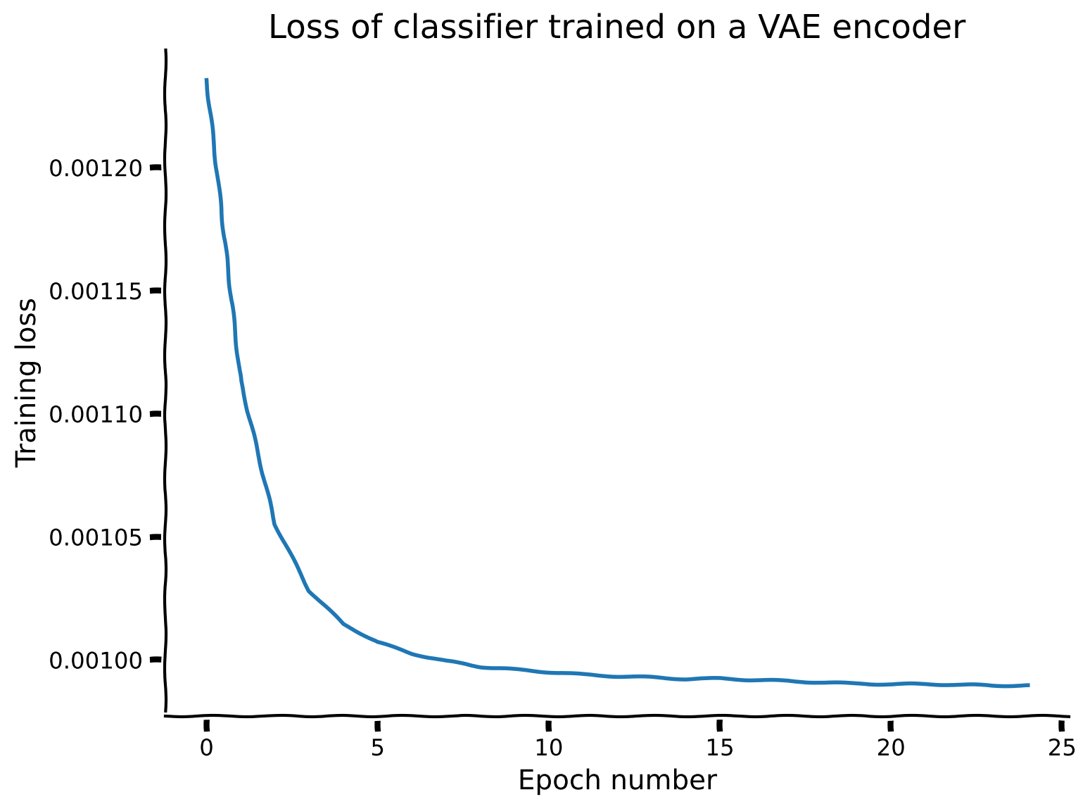
- モデル学習時に返される損失配列をプロットし、必要に応じて学習エポック数を調整する。
ヒント: は インタラクティブデモ 1.2.1 で紹介されています。
def vae_train_loss(num_epochs, seed):
  """
  Helper function to plot the train loss of the variational autoencoder (VAE)

  Args:
    num_epochs: Integer
      Number of the epochs the VAE is to be trained for
    seed: Integer
      The seed value for the dataset/network

  Returns:
    vae_loss_array: List
      Loss per epoch
  """
  # Call this before any dataset/network initializing or training,
  # to ensure reproducibility
  set_seed(seed)
  #################################################
  # Fill in missing code below (...),
  # then remove or comment the line below to test your implementation
  raise NotImplementedError("Exercise: Train a classifer on the pre-trained VAE encoder representations.")
  #################################################
  # Train an encoder and classifier on the images, using models.train_classifier()
  print("Training a classifier on the pre-trained VAE encoder representations...")
  _, vae_loss_array, _, _ = models.train_classifier(
      encoder=...,
      dataset=...,
      train_sampler=...,
      test_sampler=...,
      freeze_features=..., # Keep the encoder frozen while training the classifier
      num_epochs=...,
      verbose=... # Print results
      )
  #################################################
  # Fill in missing code below (...),
  # then remove or comment the line below to test your implementation
  raise NotImplementedError("Exercise: Plot the VAE classifier training loss.")
  #################################################
  # Plot the VAE classifier training loss.
  fig, ax = plt.subplots()
  ax.plot(...)
  ax.set_title(...)
  ax.set_xlabel(...)
  ax.set_ylabel(...)

  return vae_loss_array


# Set a reasonable number of training epochs
num_epochs = 25
## Uncomment below to test your function
# vae_loss_array = vae_train_loss(num_epochs=num_epochs, seed=SEED)
分類器の学習を25エポック行った後のネットワーク性能(チャンス: 33.33%):
訓練精度: 46.48%
テスト精度: 45.75%
出力例:
# @title Submit your feedback
content_review(f"{feedback_prefix}_Evaluate_performance_using_pretrained_VAE_Exercise")
ネットワークの損失は25エポックでかなり安定しており、その時点で分類器はテストデータセットに対して45.75%の精度を示しています。
異なる特徴エンコーダを用いた形状分類結果:
| チャンス | なし(生データ) | 教師あり | ランダム | VAE | |
|---|---|---|---|---|---|
| 33.33% | 39.55% | 98.70% | 44.67% | 45.75% |
セクション5: 不変性のための自己教師あり学習の現代的アプローチ
所要時間の目安: 約10分
# @title Video 5: Modern Approach in Self-supervised Learning
from ipywidgets import widgets
from IPython.display import YouTubeVideo
from IPython.display import IFrame
from IPython.display import display


class PlayVideo(IFrame):
  def __init__(self, id, source, page=1, width=400, height=300, **kwargs):
    self.id = id
    if source == 'Bilibili':
      src = f'https://player.bilibili.com/player.html?bvid={id}&page={page}'
    elif source == 'Osf':
      src = f'https://mfr.ca-1.osf.io/render?url=https://osf.io/download/{id}/?direct%26mode=render'
    super(PlayVideo, self).__init__(src, width, height, **kwargs)


def display_videos(video_ids, W=400, H=300, fs=1):
  tab_contents = []
  for i, video_id in enumerate(video_ids):
    out = widgets.Output()
    with out:
      if video_ids[i][0] == 'Youtube':
        video = YouTubeVideo(id=video_ids[i][1], width=W,
                             height=H, fs=fs, rel=0)
        print(f'Video available at https://youtube.com/watch?v={video.id}')
      else:
        video = PlayVideo(id=video_ids[i][1], source=video_ids[i][0], width=W,
                          height=H, fs=fs, autoplay=False)
        if video_ids[i][0] == 'Bilibili':
          print(f'Video available at https://www.bilibili.com/video/{video.id}')
        elif video_ids[i][0] == 'Osf':
          print(f'Video available at https://osf.io/{video.id}')
      display(video)
    tab_contents.append(out)
  return tab_contents


video_ids = [('Youtube', 'hUWcsSFWZyw'), ('Bilibili', 'BV1Bv411n7zP')]
tab_contents = display_videos(video_ids, W=854, H=480)
tabs = widgets.Tab()
tabs.children = tab_contents
for i in range(len(tab_contents)):
  tabs.set_title(i, video_ids[i][0])
display(tabs)
# @title Submit your feedback
content_review(f"{feedback_prefix}_Modern_approach_in_Selfsupervised_Learning_Video")セクション5.1: 不変表現学習のさまざまな選択肢の検討
ここでは、dSpritesのようなデータセットに対して不変な形状表現を学習するいくつかの方法を見ていきます。
インタラクティブデモ5.1.1: 不変性学習に使えるいくつかの画像変換の可視化
以下のコードは:
torchvision.transforms.RandomAffineクラスを使ってinvariance_transformsという変換セットを初期化し、invariance_transformsを入力として受け取り、呼び出されたときに変換を適用するtorchデータセットdSprites_invariance_torchdatasetにdSpritesデータセットをまとめ、data.dSpritesTorchDatasetのメソッドを使って画像とその変換後の例をいくつか表示します。
torchvision.transforms.RandomAffineクラスは、以下の引数を設定することで、画像変換時にどの種類の変換をどの範囲でサンプリングするかを事前に決められます:
degrees: 回転の絶対最大角度(度)translate: x方向の幅の最大移動割合とy方向の高さの最大移動割合scale: 最小から最大のスケーリング係数
インタラクティブデモ: 変換パラメータのいくつかの組み合わせを試し、同じ画像の変換ペアを可視化してみましょう。(元の設定はdegrees=90、translate=(0.2, 0.2)、scale=(0.8, 1.2)です。)
# Call this before any dataset/network initializing or training,
# to ensure reproducibility
set_seed(SEED)

# DEMO: Try some random affine data augmentations combinations to apply to the images
invariance_transforms = torchvision.transforms.RandomAffine(
    degrees=90,
    translate=(0.2, 0.2),  # (in x, in y)
    scale=(0.8, 1.2)   # min to max scaling
    )

# Initialize a simclr-specific torch dataset
dSprites_invariance_torchdataset = data.dSpritesTorchDataset(
    dSprites,
    target_latent="shape",
    simclr=True,
    simclr_transforms=invariance_transforms
    )

# Show a few example of pairs of image augmentations
_ = dSprites_invariance_torchdataset.show_images(randst=SEED)
# @title Submit your feedback
content_review(f"{feedback_prefix}_Image_transformations_Interactive_Demo")セクション6: ターゲットネットワークを用いた変換に対する不変性の学習方法
所要時間の目安: 約40分
# @title Video 6: Data Transformations
from ipywidgets import widgets
from IPython.display import YouTubeVideo
from IPython.display import IFrame
from IPython.display import display


class PlayVideo(IFrame):
  def __init__(self, id, source, page=1, width=400, height=300, **kwargs):
    self.id = id
    if source == 'Bilibili':
      src = f'https://player.bilibili.com/player.html?bvid={id}&page={page}'
    elif source == 'Osf':
      src = f'https://mfr.ca-1.osf.io/render?url=https://osf.io/download/{id}/?direct%26mode=render'
    super(PlayVideo, self).__init__(src, width, height, **kwargs)


def display_videos(video_ids, W=400, H=300, fs=1):
  tab_contents = []
  for i, video_id in enumerate(video_ids):
    out = widgets.Output()
    with out:
      if video_ids[i][0] == 'Youtube':
        video = YouTubeVideo(id=video_ids[i][1], width=W,
                             height=H, fs=fs, rel=0)
        print(f'Video available at https://youtube.com/watch?v={video.id}')
      else:
        video = PlayVideo(id=video_ids[i][1], source=video_ids[i][0], width=W,
                          height=H, fs=fs, autoplay=False)
        if video_ids[i][0] == 'Bilibili':
          print(f'Video available at https://www.bilibili.com/video/{video.id}')
        elif video_ids[i][0] == 'Osf':
          print(f'Video available at https://osf.io/{video.id}')
      display(video)
    tab_contents.append(out)
  return tab_contents


video_ids = [('Youtube', 'g6IxiUXubhM'), ('Bilibili', 'BV1H64y1t7ag')]
tab_contents = display_videos(video_ids, W=854, H=480)
tabs = widgets.Tab()
tabs.children = tab_contents
for i in range(len(tab_contents)):
  tabs.set_title(i, video_ids[i][0])
display(tabs)
# @title Submit your feedback
content_review(f"{feedback_prefix}_Data_Transformations_Video")セクション6.1: 画像変換を用いた自己教師あり学習(SSL)ネットワークでの特徴不変表現の学習
ここでは、SimCLRという特定のタイプのSSLアルゴリズムで学習したエンコーダネットワークが、どのように不変性を獲得するかを、選択する変換の違いによって比較します。具体的には、SimCLRで事前学習したエンコーダネットワークが、学習した表現を用いて訓練した分類器の性能にどのように影響するかを観察します。
コーディング演習6.1.1: SimCLR損失関数の完成
以下のコードは:
- SimCLRネットワークのコントラスト損失を計算する関数の骨組みを示し、
- カスタム関数を解答実装と比較し、
- SimCLRを数エポック訓練します。
演習:
- の実装を完成させ、
- カスタム損失関数でSimCLRを数エポック訓練した後の損失をプロットしてください。
詳細ヒント:
- :
- 2つの入力引数を取ります:
proj_feat1(2D torch Tensor): 1つ目の画像拡張の射影特徴(バッチサイズ x 特徴サイズ)proj_feat2(2D torch Tensor): 2つ目の画像拡張の射影特徴(バッチサイズ x 特徴サイズ)
- すべての画像拡張ペアの類似度行列
similarity_matrixを計算します。 similarity_matrixのインデックス指定に使う正例と負例の指標を特定します:pos_sample_indicators(2D torch Tensor): 正例画像ペアの位置を1、それ以外を0で示すテンソル(バッチサイズ×2 x バッチサイズ×2)neg_sample_indicators(2D torch Tensor): 負例画像ペアの位置を1、それ以外を0で示すテンソル(バッチサイズ×2 x バッチサイズ×2)
- 指標を用いて
similarity_matrixから値を取り出し、コントラスト損失の2つの部分を計算します:numerator: 正例ペアの類似度行列値から計算denominator: 負例ペアの類似度行列値から計算
- 2つの入力引数を取ります:
def custom_simclr_contrastive_loss(proj_feat1, proj_feat2, temperature=0.5):
  """
  Returns contrastive loss, given sets of projected features, with positive
  pairs matched along the batch dimension.

  Args:
    Required:
      proj_feat1: 2D torch.Tensor
        Projected features for first image with augmentations (size: batch_size x feat_size)
      proj_feat2: 2D torch.Tensor
        Projected features for second image with augmentations (size: batch_size x feat_size)
    Optional:
      temperature: Float
        relaxation temperature (default: 0.5)
        l2 normalization along with temperature effectively weights different
        examples, and an appropriate temperature can help the model learn from hard negatives.
  Returns:
    loss: Float
      Mean contrastive loss
  """
  device = proj_feat1.device

  if len(proj_feat1) != len(proj_feat2):
    raise ValueError(f"Batch dimension of proj_feat1 ({len(proj_feat1)}) "
                     f"and proj_feat2 ({len(proj_feat2)}) should be same")

  batch_size = len(proj_feat1) # N
  z1 = torch.nn.functional.normalize(proj_feat1, dim=1)
  z2 = torch.nn.functional.normalize(proj_feat2, dim=1)

  proj_features = torch.cat([z1, z2], dim=0) # 2N x projected feature dimension
  similarity_matrix = torch.nn.functional.cosine_similarity(
      proj_features.unsqueeze(1), proj_features.unsqueeze(0), dim=2
      ) # dim: 2N x 2N

  # Initialize arrays to identify sets of positive and negative examples, of
  # shape (batch_size * 2, batch_size * 2), and where
  # 0 indicates that 2 images are NOT a pair (either positive or negative, depending on the indicator type)
  # 1 indices that 2 images ARE a pair (either positive or negative, depending on the indicator type)
  pos_sample_indicators = torch.roll(torch.eye(2 * batch_size), batch_size, 1).to(device)
  neg_sample_indicators = (torch.ones(2 * batch_size) - torch.eye(2 * batch_size)).to(device)

  #################################################
  # Fill in missing code below (...),
  # then remove or comment the line below to test your function
  raise NotImplementedError("Exercise: Implement SimCLR loss.")
  #################################################
  # Implement the SimClr loss calculation
  # Calculate the numerator of the Loss expression by selecting the appropriate elements from similarity_matrix.
  # Use the pos_sample_indicators tensor
  numerator = ...

  # Calculate the denominator of the Loss expression by selecting the appropriate elements from similarity_matrix,
  # and summing over pairs for each item.
  # Use the neg_sample_indicators tensor
  denominator = ...

  if (denominator < 1e-8).any(): # Clamp to avoid division by 0
    denominator = torch.clamp(denominator, 1e-8)

  loss = torch.mean(-torch.log(numerator / denominator))

  return loss


## Uncomment below to test your function
# test_custom_contrastive_loss_fct(custom_simclr_contrastive_loss)
custom_simclr_contrastive_loss() は正しく実装されています。
# @title Submit your feedback
content_review(f"{feedback_prefix}_SimCLR_loss_function_Exercise")
これでカスタムコントラスト損失を用いてSimCLRエンコーダを数エポック訓練できます。
# Call this before any dataset/network initializing or training,
# to ensure reproducibility
set_seed(SEED)

# Train SimCLR for a few epochs
print("Training a SimCLR encoder with the custom contrastive loss...")
num_epochs = 5
_, test_simclr_loss_array = models.train_simclr(
    encoder=models.EncoderCore(),
    dataset=dSprites_invariance_torchdataset,
    train_sampler=train_sampler,
    num_epochs=num_epochs,
    loss_fct=custom_simclr_contrastive_loss
    )

# Plot SimCLR loss over a few epochs.
fig, ax = plt.subplots()
ax.plot(test_simclr_loss_array)
ax.set_title("SimCLR network loss")
ax.set_xlabel("Epoch number")
_ = ax.set_ylabel("Training loss")自己教師ありモデルは通常、教師ありモデルよりも多くの訓練を必要とするため、ここでは完全に事前学習する代わりに、60エポック事前学習済みのモデルを読み込みます。エンコーダは、上記の教師あり、ランダム、VAEの例と同じアーキテクチャを共有しています。
以下のコードは:
- を使ってSimCLRコントラストタスクで事前学習済みのSimCLRネットワークのパラメータを読み込みます。
# Load SimCLR encoder pre-trained on the contrastive loss
simclr_encoder = load.load_encoder(REPO_PATH, model_type="simclr")
インタラクティブデモ6.1.1: 事前学習済みSimCLRエンコーダの表現で訓練したロジスティック回帰の分類性能評価
事前学習済みSimCLRエンコーダはVAEエンコーダと同様に、パラメータがすでに学習済みなので、分類器訓練時にはfreeze_features=Trueで凍結します。
分類器の訓練とテストはdSprites_invariance_torchdatasetではなくdSprites_torchdatasetで行います。これは、拡張画像ではなく実際のdSprites画像での分類器性能を評価したいためです。
インタラクティブデモ: 分類器の訓練エポック数を変えて試してみましょう。(元の設定はnum_epochs=10です。)
# Call this before any dataset/network initializing or training,
# to ensure reproducibility
set_seed(SEED)

print("Training a classifier on the pre-trained SimCLR encoder representations...")
_, simclr_loss_array, _, _ = models.train_classifier(
    encoder=simclr_encoder,
    dataset=dSprites_torchdataset,
    train_sampler=train_sampler,
    test_sampler=test_sampler,
    freeze_features=True,  # Keep the encoder frozen while training the classifier
    num_epochs=10,  # DEMO: Try different numbers of epochs
    verbose=True
    )

fig, ax = plt.subplots()
ax.plot(simclr_loss_array)
ax.set_title("Loss of classifier trained on a SimCLR encoder.")
ax.set_xlabel("Epoch number")
_ = ax.set_ylabel("Training loss")
分類器訓練10エポック後のネットワーク性能(チャンス: 33.33%):
訓練精度: 97.83%
テスト精度: 97.53%
# @title Submit your feedback
content_review(f"{feedback_prefix}_Evaluate_performance_using_pretrained_SimCLR_Interactive_Demo")
上記の変換を用いたネットワークは、15エポックの分類器訓練後にテストデータセットで97.53%の精度を示します。
異なる特徴エンコーダを用いた形状分類結果:
| チャンス | なし(生データ) | 教師あり | ランダム | VAE | SimCLR | |
|---|---|---|---|---|---|---|
| 33.33% | 39.55% | 98.70% | 44.67% | 45.75% | 97.53% |
セクション7: バイアスのあるデータセットからの自己教師あり学習に関する倫理的考察
# @title Video 7: Un/Self-Supervised Learning
from ipywidgets import widgets
from IPython.display import YouTubeVideo
from IPython.display import IFrame
from IPython.display import display


class PlayVideo(IFrame):
  def __init__(self, id, source, page=1, width=400, height=300, **kwargs):
    self.id = id
    if source == 'Bilibili':
      src = f'https://player.bilibili.com/player.html?bvid={id}&page={page}'
    elif source == 'Osf':
      src = f'https://mfr.ca-1.osf.io/render?url=https://osf.io/download/{id}/?direct%26mode=render'
    super(PlayVideo, self).__init__(src, width, height, **kwargs)


def display_videos(video_ids, W=400, H=300, fs=1):
  tab_contents = []
  for i, video_id in enumerate(video_ids):
    out = widgets.Output()
    with out:
      if video_ids[i][0] == 'Youtube':
        video = YouTubeVideo(id=video_ids[i][1], width=W,
                             height=H, fs=fs, rel=0)
        print(f'Video available at https://youtube.com/watch?v={video.id}')
      else:
        video = PlayVideo(id=video_ids[i][1], source=video_ids[i][0], width=W,
                          height=H, fs=fs, autoplay=False)
        if video_ids[i][0] == 'Bilibili':
          print(f'Video available at https://www.bilibili.com/video/{video.id}')
        elif video_ids[i][0] == 'Osf':
          print(f'Video available at https://osf.io/{video.id}')
      display(video)
    tab_contents.append(out)
  return tab_contents


video_ids = [('Youtube', 'NT006a6nkyg'), ('Bilibili', 'BV1mP4y1473E')]
tab_contents = display_videos(video_ids, W=854, H=480)
tabs = widgets.Tab()
tabs.children = tab_contents
for i in range(len(tab_contents)):
  tabs.set_title(i, video_ids[i][0])
display(tabs)
# @title Submit your feedback
content_review(f"{feedback_prefix}_Un_self_supervised_learning_Video")セクション7.1: バイアスのあるデータセットでモデルを訓練した場合の影響
モデルがバイアスのあるデータセットで訓練されると、そのバイアスを再現する表現エンコーディングを学習しやすくなり、適切に一般化できなくなり、バイアスをさらに拡散する可能性が高まります。
ここでは、訓練データセットのバイアスのあるサブセットでモデルを訓練した場合の影響を調べます。具体的には、train_sampler_biasedという訓練データセットサンプラーを導入し、以下のみをサンプリングします:
- 画像の左側に中心がある場合の四角形(posX: 0〜0.3)、
- 画像の中央に中心がある場合の楕円(posX: 0.35〜0.65)、
- 画像の右側に中心がある場合のハート(posX: 0.7〜1.0)。
このサンプリングバイアスは、元のデータセットにはないshapeとposXの相関を導入します。
その後、各モデルを上記のように訓練し、バイアスのないデータセットでテストしたときの性能を観察します。
データセットサイズについての注意: このバイアス付きサンプリングは訓練データセットのサイズを大幅に減少させます(約6分の1)。したがって、ここでの結果をチュートリアルの前の結果と比較するのは公平ではありません。このため、対照として、train_sampler_bias_ctrlというバイアスのないサンプラーでも同じサンプル数だけ訓練を行います。
# Call this before any dataset/network initializing or training,
# to ensure reproducibility
set_seed(SEED)

bias_type = "shape_posX_spaced"  # Name of bias

# Initialize a biased training sampler and an unbiased test sampler
train_sampler_biased, test_sampler_for_biased = data.train_test_split_idx(
    dSprites_torchdataset,
    fraction_train=0.95,  # 95:5 Split to partially compensate for loss of training examples due to bias
    randst=SEED,
    train_bias=bias_type
    )

# Initialize a control, unbiased training sampler and an unbiased test sampler
train_sampler_bias_ctrl, test_sampler_for_bias_ctrl = data.train_test_split_idx(
    dSprites_torchdataset,
    fraction_train=0.95,
    randst=SEED,
    train_bias=bias_type,
    control=True
    )

print(f"Biased dataset: {len(train_sampler_biased)} training, "
      f"{len(test_sampler_for_biased)} test images")
print(f"Bias control dataset: {len(train_sampler_bias_ctrl)} training, "
f"{len(test_sampler_for_bias_ctrl)} test images")train_sampler_biasedでサンプリングした画像をプロットし、shapeとposXが相関しているパターンを観察します。
バイアスをより視覚的に理解するために、赤色で以下の注釈を付けてプロットします:
- 3つの
posX区間の境界線 - 各形状の中心(
posX,posY)
print("Plotting first 20 images from the biased training dataset.\n")
dSprites.show_images(indices=train_sampler_biased.indices[:20], annotations="posX_quadrants")train_sampler_bias_ctrlでサンプリングした画像もプロットし、対照データセットにバイアスパターンが現れないことを視覚的に確認します。
こちらも注釈は視覚化のためだけに追加しています。
print("Plotting sample images from the bias control training dataset.\n")
dSprites.show_images(indices=train_sampler_bias_ctrl.indices[:20], annotations="posX_quadrants")
# @markdown ### Function to run full training procedure
# @markdown (from initializing and pretraining encoders to training classifiers):
# @markdown `full_training_procedure(train_sampler, test_sampler)`
def full_training_procedure(train_sampler, test_sampler, title=None,
dataset_type="biased", verbose=True):
"""
Funtion to load pretrained VAE and SimCLR encoders
Args:
train_sampler: torch.Tensor
Training Data
test_sampler: torch.Tensor
Test Data
title: String
Title
dataset_type: String
Specifies if the expected model type is biased/bias-controlled
verbose: Boolean
If true, the shell shows all lines in the script in execution
Returns:
Nothing
"""
if dataset_type not in ["biased", "bias_ctrl"]:
raise ValueError("Expected model_type to be 'biased' or 'bias_ctrl', "
f"but found {model_type}.")
supervised_encoder = models.EncoderCore()
random_encoder = models.EncoderCore()
# Load pre-trained VAE
vae_encoder = load.load_encoder(
REPO_PATH, model_type="vae", dataset_type=dataset_type,
verbose=verbose
)
# Load pre-trained SimCLR encoder
simclr_encoder = load.load_encoder(
REPO_PATH, model_type="simclr", dataset_type=dataset_type,
verbose=verbose
)
encoders = [supervised_encoder, random_encoder, vae_encoder, simclr_encoder]
freeze_features = [False, True, True, True]
encoder_labels = ["supervised", "random", "VAE", "SimCLR"]
num_clf_epochs = [80, 30, 30, 30]
print(f"\nTraining supervised encoder and classifier for {num_clf_epochs[0]} "
f"epochs, and all other classifiers for {num_clf_epochs[1]} epochs each.")
_ = models.train_encoder_clfs_by_fraction_labelled(
encoders=encoders,
dataset=dSprites_torchdataset,
train_sampler=train_sampler,
test_sampler=test_sampler,
num_epochs=num_clf_epochs,
freeze_features=freeze_features,
subset_seed=SEED,
encoder_labels=encoder_labels,
title=title,
verbose=verbose
)ここでは、バイアスのある訓練データサンプラー(とバイアスのない対照サンプラー)を用いて、異なるモデルの性能を観察します。データセットが小さいため、エンコーダと分類器の事前学習および訓練エポック数を増やします。
まずはバイアスのない対照サンプラーで、データセットサイズに応じた分類性能の目安を確認しましょう。
# Call this before any dataset/network initializing or training,
# to ensure reproducibility
set_seed(SEED)

print("Training all models using the control, unbiased training dataset\n")
full_training_procedure(
    train_sampler_bias_ctrl, test_sampler_for_bias_ctrl,
    title="Classifier performances with control, unbiased training dataset",
    dataset_type="bias_ctrl"  # For loading correct pre-trained networks
    )
フルデータセットの場合と似たパターンが観察されますが、ほとんどの性能がやや低下しています。これは、(A) 訓練データセットが小さいこと、(B) 時間効率のためにエポック数を少なくしていることが原因と考えられます。
同じパラメータで、バイアスのある訓練データサンプラーで分析を繰り返します。
# Call this before any dataset/network initializing or training,
# to ensure reproducibility
set_seed(SEED)

print("Training all models using the biased training dataset\n")
full_training_procedure(
    train_sampler_biased, test_sampler_for_biased,
    title="Classifier performances with biased training dataset",
    dataset_type="biased"  # For loading correct pre-trained networks
    )
興味深いことに、SimCLRネットワークエンコーダは唯一良好な性能を示すだけでなく、この特定のデータセットとバイアス条件下では対照性能(同じテストデータセットを用いたもの)を上回っています。
_性能向上についての注意: SimCLRエンコーダのこの性能向上は、事前学習損失曲線(ここでは示していません)にも反映されており、バイアス付きデータセットで訓練したエンコーダはバイアスなし訓練セットよりも速く学習しています。データセットのバイアスにより変動性が減り、コントラストタスクが容易になって、少ないエポックで良い特徴空間を学習できた可能性があります。
議論7.1.1: バイアスのある訓練データセットに対して異なるモデルはどのように対処するか?
A. バイアスのある訓練データセットに最も影響を受けやすいモデルと最も影響を受けにくいモデルはどれか?
B. テストセットのどのタイプの画像が性能低下の主な原因となっているか?
C. なぜ特定のモデルはここで導入されたバイアスに対してより頑健なのか?
D. モデルが良いデータ表現を学習する能力に対する訓練セットのバイアスの悪影響を軽減するためにどのような方法が考えられるか?
# @title Submit your feedback
content_review(f"{feedback_prefix}_Biased_training_dataset_Discussion")
議論7.1.2: これらの原則はより一般的にどのように適用されるか?
自己教師あり学習(SSL)がネットワークの良いデータ表現学習能力を向上させることを見てきました。本チュートリアルでは、以下のような単純化されたデータセットで例を示しました:
(1) すべての画像の潜在次元が既知で、
(2) 全データセットの潜在次元間の結合確率分布がわかり、
(3) バイアス付きデータセットに導入されたバイアスの性質が正確にわかっている(詳細はボーナス2参照)。
そのため、事前学習エンコーダが下流の分類タスクに適した良い特徴空間を学習するようなデータ拡張を設計するのは比較的簡単です。
実際の応用では、より複雑または困難なデータセットに対して、
A. SSLを用いて良いデータ表現を学習するためにどのような原則を適用できるか?例えば、
B. dSpritesに比べて新しいデータセットでSSLを適用する際にどのような課題があるか?
C. 音声データセットのような非視覚的データセットに対してはどのような拡張を使うか?また、本チュートリアルでは主にSimCLRという1種類のSSLを扱いましたが、明示的なデータ拡張を使わないSSLも存在します。
D. 時系列データに対してどのようなSSLタスクを実装できるか?例えば、脳波記録から睡眠段階を予測したい場合、睡眠段階が時間的にゆっくり変化することを利用してどのようなSSLタスクを構築できるか?
# @title Submit your feedback
content_review(f"{feedback_prefix}_General_Principles_Discussion")
まとめ
# @title Video 8: Conclusion
from ipywidgets import widgets
from IPython.display import YouTubeVideo
from IPython.display import IFrame
from IPython.display import display


class PlayVideo(IFrame):
  def __init__(self, id, source, page=1, width=400, height=300, **kwargs):
    self.id = id
    if source == 'Bilibili':
      src = f'https://player.bilibili.com/player.html?bvid={id}&page={page}'
    elif source == 'Osf':
      src = f'https://mfr.ca-1.osf.io/render?url=https://osf.io/download/{id}/?direct%26mode=render'
    super(PlayVideo, self).__init__(src, width, height, **kwargs)


def display_videos(video_ids, W=400, H=300, fs=1):
  tab_contents = []
  for i, video_id in enumerate(video_ids):
    out = widgets.Output()
    with out:
      if video_ids[i][0] == 'Youtube':
        video = YouTubeVideo(id=video_ids[i][1], width=W,
                             height=H, fs=fs, rel=0)
        print(f'Video available at https://youtube.com/watch?v={video.id}')
      else:
        video = PlayVideo(id=video_ids[i][1], source=video_ids[i][0], width=W,
                          height=H, fs=fs, autoplay=False)
        if video_ids[i][0] == 'Bilibili':
          print(f'Video available at https://www.bilibili.com/video/{video.id}')
        elif video_ids[i][0] == 'Osf':
          print(f'Video available at https://osf.io/{video.id}')
      display(video)
    tab_contents.append(out)
  return tab_contents


video_ids = [('Youtube', 'tvZzYfi_bTI'), ('Bilibili', 'BV1Tq4y1X7e1')]
tab_contents = display_videos(video_ids, W=854, H=480)
tabs = widgets.Tab()
tabs.children = tab_contents
for i in range(len(tab_contents)):
  tabs.set_title(i, video_ids[i][0])
display(tabs)
# @title Submit your feedback
content_review(f"{feedback_prefix}_Conclusion_Video")ボーナス1: 自己教師ありネットワークは表現の不変性を学習する
所要時間の目安: 約20分
# @title Video 9: Invariant Representations
from ipywidgets import widgets
from IPython.display import YouTubeVideo
from IPython.display import IFrame
from IPython.display import display


class PlayVideo(IFrame):
  def __init__(self, id, source, page=1, width=400, height=300, **kwargs):
    self.id = id
    if source == 'Bilibili':
      src = f'https://player.bilibili.com/player.html?bvid={id}&page={page}'
    elif source == 'Osf':
      src = f'https://mfr.ca-1.osf.io/render?url=https://osf.io/download/{id}/?direct%26mode=render'
    super(PlayVideo, self).__init__(src, width, height, **kwargs)


def display_videos(video_ids, W=400, H=300, fs=1):
  tab_contents = []
  for i, video_id in enumerate(video_ids):
    out = widgets.Output()
    with out:
      if video_ids[i][0] == 'Youtube':
        video = YouTubeVideo(id=video_ids[i][1], width=W,
                             height=H, fs=fs, rel=0)
        print(f'Video available at https://youtube.com/watch?v={video.id}')
      else:
        video = PlayVideo(id=video_ids[i][1], source=video_ids[i][0], width=W,
                          height=H, fs=fs, autoplay=False)
        if video_ids[i][0] == 'Bilibili':
          print(f'Video available at https://www.bilibili.com/video/{video.id}')
        elif video_ids[i][0] == 'Osf':
          print(f'Video available at https://osf.io/{video.id}')
      display(video)
    tab_contents.append(out)
  return tab_contents


video_ids = [('Youtube', 'f8FCk519-lI'), ('Bilibili', 'BV1Ry4y1L7Hz')]
tab_contents = display_videos(video_ids, W=854, H=480)
tabs = widgets.Tab()
tabs.children = tab_contents
for i in range(len(tab_contents)):
  tabs.set_title(i, video_ids[i][0])
display(tabs)
# @title Submit your feedback
content_review(f"{feedback_prefix}_Invariant_Representations_Bonus_Video")ボーナス1.1: SimCLRネットワーク表現におけるデータ変換の不変性への影響
事前学習済みSimCLRネットワークエンコーダにデータ変換を加えた場合の不変性への影響を観察します。
ボーナスインタラクティブデモ1.1.1: 異なる潜在次元に沿って整理したSimCLRネットワークエンコーダのRSMの可視化
事前学習済みSimCLRエンコーダのRSMを、これまで生成したエンコーダRSMと比較します。
ここでもdSprites_invariance_torchdatasetではなくdSprites_torchdatasetを渡します。これは実際のdSprites画像のRSMに興味があるためです。
インタラクティブデモ: RSMを異なる潜在次元("scale"、"orientation"、"posX"、"posY")に沿って可視化し、異なるエンコーダネットワークで観察されるパターンを比較しましょう。(元の設定はsorting_latent="shape"です。)
sorting_latent = "shape"  # DEMO: Try sorting by different latent dimensions
print("Plotting RSMs...")
_ = models.plot_model_RSMs(
    encoders=[supervised_encoder, vae_encoder, simclr_encoder],
    dataset=dSprites_torchdataset,
    sampler=test_sampler,  # To see the representations on the held out test set
    titles=["Supervised network encoder RSM", "VAE network encoder RSM",
            "SimCLR network encoder RSM"],  # Plot titles
    sorting_latent=sorting_latent
    )
# @title Submit your feedback
content_review(f"{feedback_prefix}_SimCLR_network_encoder_RSMs_Bonus_Interactive_Demo")ボーナス議論1.1.1: SimCLRのようなコントラストモデルが意味のある表現空間を構築できる能力について何が言えるか?
A. 事前学習済みSimCLRエンコーダのRSM(異なる潜在次元でソート)と教師ありおよび事前学習済みVAEエンコーダのRSMはどう比較されるか?
B. これらの異なるRSMは何によって説明されるか?
C. いくつかのエンコーダが他よりも持つ利点は何か?
D. SimCLRエンコーダがコントラストタスクで良い性能を示すことは、下流の分類タスクでの良い性能を保証するか?
E. 例えば、下流タスクがorientation予測の場合、SimCLRエンコーダの事前学習をどのように変更できるか?
# @markdown #### Supporting images for Discussion response examples for Bonus 1.1.1: All SimCLR encoder RSMs
Image(filename=os.path.join(REPO_PATH, "images", "rsms_simclr_encoder_60ep_bs1000_deg90_trans0-2_scale0-8to1-2_seed2021.png"), width=1000)# @title Submit your feedback
content_review(f"{feedback_prefix}_Contrastive_models_Bonus_Discussion")ボーナス2: 表現の崩壊を避ける
# @title Video 10: Avoiding Representational Collapse
from ipywidgets import widgets
from IPython.display import YouTubeVideo
from IPython.display import IFrame
from IPython.display import display


class PlayVideo(IFrame):
  def __init__(self, id, source, page=1, width=400, height=300, **kwargs):
    self.id = id
    if source == 'Bilibili':
      src = f'https://player.bilibili.com/player.html?bvid={id}&page={page}'
    elif source == 'Osf':
      src = f'https://mfr.ca-1.osf.io/render?url=https://osf.io/download/{id}/?direct%26mode=render'
    super(PlayVideo, self).__init__(src, width, height, **kwargs)


def display_videos(video_ids, W=400, H=300, fs=1):
  tab_contents = []
  for i, video_id in enumerate(video_ids):
    out = widgets.Output()
    with out:
      if video_ids[i][0] == 'Youtube':
        video = YouTubeVideo(id=video_ids[i][1], width=W,
                             height=H, fs=fs, rel=0)
        print(f'Video available at https://youtube.com/watch?v={video.id}')
      else:
        video = PlayVideo(id=video_ids[i][1], source=video_ids[i][0], width=W,
                          height=H, fs=fs, autoplay=False)
        if video_ids[i][0] == 'Bilibili':
          print(f'Video available at https://www.bilibili.com/video/{video.id}')
        elif video_ids[i][0] == 'Osf':
          print(f'Video available at https://osf.io/{video.id}')
      display(video)
    tab_contents.append(out)
  return tab_contents


video_ids = [('Youtube', 'fS2BAKVdpIY'), ('Bilibili', 'BV1Gv411E7xe')]
tab_contents = display_videos(video_ids, W=854, H=480)
tabs = widgets.Tab()
tabs.children = tab_contents
for i in range(len(tab_contents)):
  tabs.set_title(i, video_ids[i][0])
display(tabs)
# @title Submit your feedback
content_review(f"{feedback_prefix}_Avoiding_Representational_Collapse_Bonus_Video")ボーナス2.1: SimCLRコントラスト損失で負例の数を減らした場合の影響
上記のコントラスト損失実装で見たように、コントラスト損失でニューラルネットワークを訓練する戦略として、大きなバッチサイズ(ここでは1,000例)を使い、バッチ内の異なる画像の表現を互いの負例として用います。つまり、バッチサイズ1,000なら各画像は1つの正例ペア(対応する拡張画像)と999の負例ペア(自身以外のすべての画像、対応拡張も含む)を持ち、これにより類似度分布の良い推定が可能になります。
負例を少なくした場合の影響を観察するため、負例ペア数をneg_pairs=2に設定して事前学習したSimCLRネットワークを使います。このパラメータは損失計算時に各画像で利用する負例ペアを2つだけに制限します。
以下のコードは:
- を使って、負例ペアを2つだけ使ってSimCLRコントラストタスクで事前学習したSimCLRネットワークのパラメータを読み込み、
- 比較のためにいくつかのネットワークエンコーダのRSMをプロットします。
# Call this before any dataset/network initializing or training,
# to ensure reproducibility
set_seed(SEED)

# Load SimCLR encoder pre-trained on the contrastive loss
simclr_encoder_neg_pairs = load.load_encoder(
    REPO_PATH, model_type="simclr", neg_pairs=2
    )
ボーナスコーディング演習2.1.1: 異なる潜在次元に沿って整理したネットワークエンコーダRSMの可視化と類似度ヒストグラムのプロット
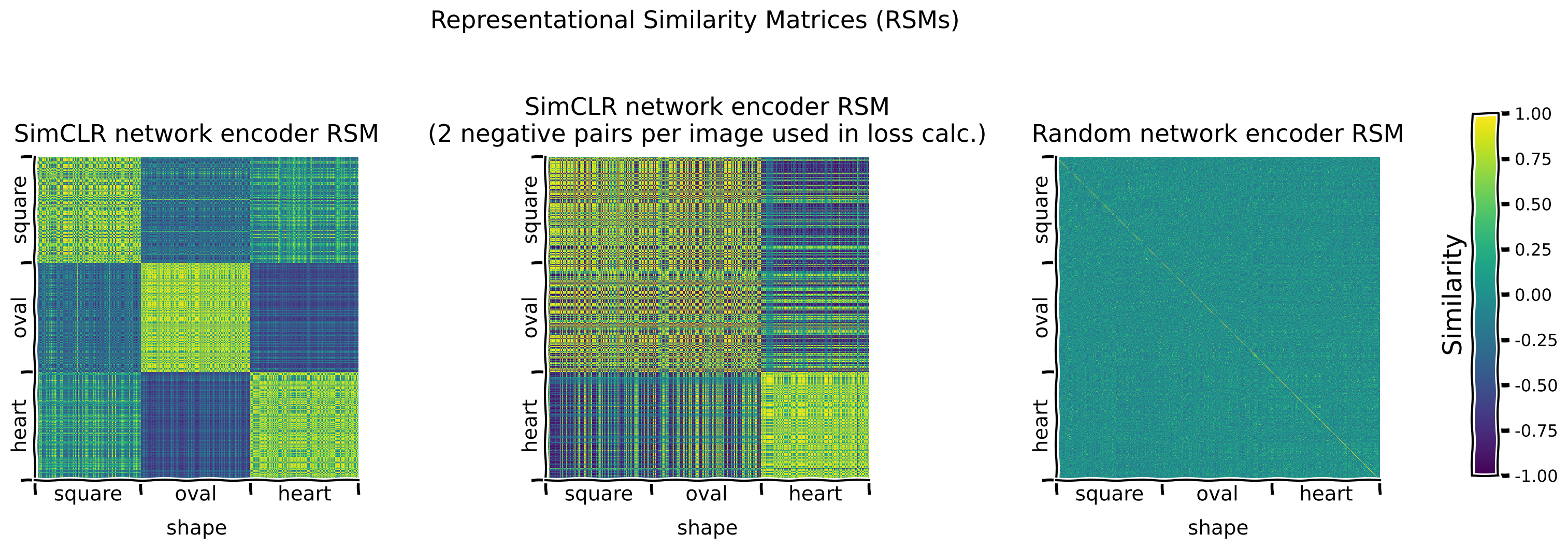
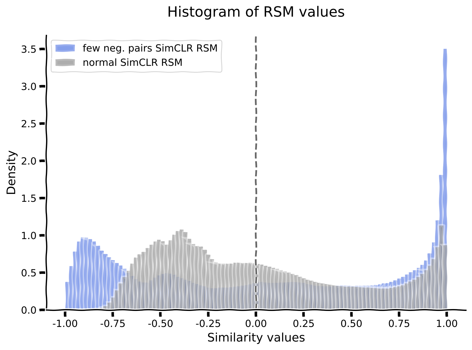
負例ペアを2つだけ使って事前学習したSimCLRエンコーダのRSMを、通常のSimCLRエンコーダとランダムエンコーダのRSMと比較します。比較のために、両者のRSM値のヒストグラムもプロットします。
演習:
shape潜在次元に沿ってRSMを可視化し、異なるエンコーダで観察されるパターンを比較する。- 通常のSimCLRと2-neg-pair SimCLRエンコーダのRSM値のヒストグラムをプロットする。
ヒント:
- は各エンコーダのRSMのデータ行列を返します。
def rsms_and_histogram_plot():
  """
  Function to plot Representational Similarity Matrices (RSMs) and Histograms

  Args:
    None

  Returns:
    Nothing
  """
  sorting_latent = "shape" # Exercise: Try sorting by different latent dimensions
  # EXERCISE: Visualize RSMs for the normal SimCLR, 2-neg-pair SimCLR and random network encoders.
  print("Plotting RSMs...")
  simclr_rsm, simclr_neg_pairs_rsm, random_rsm = models.plot_model_RSMs(
      encoders=[simclr_encoder, simclr_encoder_neg_pairs, random_encoder],
      dataset=dSprites_torchdataset,
      sampler=test_sampler, # To see the representations on the held out test set
      titles=["SimCLR network encoder RSM",
              f"SimCLR network encoder RSM\n(2 negative pairs per image used in loss calc.)",
              "Random network encoder RSM"], # Plot titles
      sorting_latent=sorting_latent
      )
  #################################################
  # Fill in missing code below (...),
  # then remove or comment the line below to test your implementation
  raise NotImplementedError("Exercise: Plot histogram.")
  #################################################
  # Plot a histogram of RSM values for both SimCLR encoders.
  plot_rsm_histogram(
      [..., ...],
      colors=[...],
      labels=[..., ...],
      nbins=100
      )


## Uncomment below to test your code
# rsms_and_histogram_plot()出力例:
# @title Submit your feedback
content_review(f"{feedback_prefix}_Visualizing_the_network_encoder_RSMs_Bonus_Exercise")
ボーナスインタラクティブデモ2.1.1: 負例ペア数を制限して事前学習したSimCLRエンコーダの表現で訓練したロジスティック回帰の分類性能評価
2-neg-pair SimCLRエンコーダもパラメータは事前学習済みなので、分類器訓練時にはfreeze_features=Trueで凍結します。
インタラクティブデモ: 分類器の訓練エポック数を変えて試してみましょう。(元の設定はnum_epochs=25です。)
# Call this before any dataset/network initializing or training,
# to ensure reproducibility
set_seed(SEED)
print("Training a classifier on the representations learned by the SimCLR "
      "network encoder pre-trained\nusing only 2 negative pairs per image "
      "for the loss calculation...")
_, simclr_neg_pairs_loss_array, _, _ = models.train_classifier(
    encoder=simclr_encoder_neg_pairs,
    dataset=dSprites_torchdataset,
    train_sampler=train_sampler,
    test_sampler=test_sampler,
    freeze_features=True,  # Keep the encoder frozen while training the classifier
    num_epochs=50,  # DEMO: Try different numbers of epochs
    verbose=True
    )

# Plot the loss array
fig, ax = plt.subplots()
ax.plot(simclr_neg_pairs_loss_array)
ax.set_title(("Loss of classifier trained on a SimCLR encoder\n"
"trained with 2 negative pairs only."))
ax.set_xlabel("Epoch number")
_ = ax.set_ylabel("Training loss")
ボーナス議論2.1.1: SimCLRのようなモデルのコントラスト損失計算における負例ペアの重要性について何が言えるか?
A. 負例ペア数を変えるとネットワークのRSMはどう変わるか?
B. 負例ペアが非常に少ない場合、エンコーダの事前学習後の形状分類器の性能はどうなるか?
C. 直感的に、負例ペアはコントラストモデルが学習する特徴空間の形成にどのような役割を果たし、正例ペアの役割とどう関係するか?
# @markdown #### Supporting images for Discussion response examples for Bonus 2.1.1: All SimCLR encoder (2 neg. pairs) RSMs
Image(filename=os.path.join(REPO_PATH, "images", "rsms_simclr_encoder_2neg_60ep_bs1000_deg90_trans0-2_scale0-8to1-2_seed2021.png"), width=1000)# @title Submit your feedback
content_review(f"{feedback_prefix}_Negative_pairs_in_computing_the_contrastive_loss_Bonus_Discussion")# @title Submit your feedback
content_review(f"{feedback_prefix}_SimCLR_network_encoder_pretrained_with_only_a_few_negative_pairs_Bonus_Interactive_Demo")SimCLRエンコーダの事前学習で使用する負例ペア数を減らした結果、分類器の訓練を50エポック行ってもテストデータセットでの分類精度は66.75%に低下しました。
異なる特徴エンコーダを用いた形状分類結果:
| チャンス | なし(生データ) | 教師あり | ランダム | VAE | SimCLR | SimCLR(負例ペア少数) | |
|---|---|---|---|---|---|---|---|
| 33.33% | 39.55% | 98.70% | 44.67% | 45.75% | 97.53% | 66.75% |
ボーナス3: 良い表現は少数ショット学習を可能にする
# @title Video 11: Few-shot Supervised Learning
from ipywidgets import widgets
from IPython.display import YouTubeVideo
from IPython.display import IFrame
from IPython.display import display


class PlayVideo(IFrame):
  def __init__(self, id, source, page=1, width=400, height=300, **kwargs):
    self.id = id
    if source == 'Bilibili':
      src = f'https://player.bilibili.com/player.html?bvid={id}&page={page}'
    elif source == 'Osf':
      src = f'https://mfr.ca-1.osf.io/render?url=https://osf.io/download/{id}/?direct%26mode=render'
    super(PlayVideo, self).__init__(src, width, height, **kwargs)


def display_videos(video_ids, W=400, H=300, fs=1):
  tab_contents = []
  for i, video_id in enumerate(video_ids):
    out = widgets.Output()
    with out:
      if video_ids[i][0] == 'Youtube':
        video = YouTubeVideo(id=video_ids[i][1], width=W,
                             height=H, fs=fs, rel=0)
        print(f'Video available at https://youtube.com/watch?v={video.id}')
      else:
        video = PlayVideo(id=video_ids[i][1], source=video_ids[i][0], width=W,
                          height=H, fs=fs, autoplay=False)
        if video_ids[i][0] == 'Bilibili':
          print(f'Video available at https://www.bilibili.com/video/{video.id}')
        elif video_ids[i][0] == 'Osf':
          print(f'Video available at https://osf.io/{video.id}')
      display(video)
    tab_contents.append(out)
  return tab_contents


video_ids = [('Youtube', 'okrvQDeN2cc'), ('Bilibili', 'BV1BP4y147fs')]
tab_contents = display_videos(video_ids, W=854, H=480)
tabs = widgets.Tab()
tabs.children = tab_contents
for i in range(len(tab_contents)):
  tabs.set_title(i, video_ids[i][0])
display(tabs)
# @title Submit your feedback
content_review(f"{feedback_prefix}_FewShot_Supervised_learning_Bonus_Video")ボーナス3.1: ラベル付き例が少ない場合にエンコーダを事前学習する利点
これまで使ってきたおもちゃデータセットdSpritesは5つの異なる次元に沿って完全にラベル付けされていますが、多くのデータセットはそうではありません。非常に大きなデータセットでもラベルがほとんどない場合があります。
最後に、ラベル付き画像が少数しかない場合に各モデルがどのように性能を発揮するかを調べます。このシナリオでは、訓練データの異なる割合(0.01〜1.0)で分類器を訓練し、テストセットでの性能を評価します。
異なるエンコーダタイプについては:
- 教師ありエンコーダ: 教師ありエンコーダはラベル付きでしか訓練できないため、ランダムエンコーダから始めて、許可されたラベル付き画像の割合で分類タスクをエンドツーエンドで訓練します。
注意: ネットワークをエンドツーエンドで訓練するため、エポック数を多くし、グラフでは"*"で示します。 - ランダムエンコーダ: 定義上、ランダムエンコーダは未訓練です。
- VAEエンコーダ: 生成モデルとしてラベルなしデータで事前学習できるため、全データセットで再構成タスクで事前学習したVAEエンコーダを使い、その後許可されたラベル付き画像の割合で分類器層を訓練します。
- SimCLRエンコーダ: SSLモデルとしてラベルなしデータで事前学習できるため、全データセットでコントラストタスクで事前学習したSimCLRエンコーダを使い、その後許可されたラベル付き画像の割合で分類器層を訓練します。
_訓練エポック数について: 以下のエポック数は全訓練データセット使用時のものです。訓練データの割合が減るにつれて、訓練エポック数は補正して増やします。例えば、10エポック指定なら0.1割合の分類器は約30エポック訓練します。また、時間の都合で上記よりやや少なめのエポック数を使います。
ボーナスインタラクティブデモ3.1.1: フルラベル付きデータセットの一部だけを使って異なるエンコーダの分類器を訓練
このデモでは、フルラベル付きデータセットの4〜6個の割合を選択して分類器を訓練します。
インタラクティブデモ: labelled_fractions引数に0.01〜1.0の間の4〜6個の割合をリストで指定し、各エンコーダの分類器を訓練してください。
# Call this before any dataset/network initializing or training,
# to ensure reproducibility
set_seed(SEED)

new_supervised_encoder = models.EncoderCore()  # New, random supervised encoder

_ = models.train_encoder_clfs_by_fraction_labelled(
    encoders=[new_supervised_encoder, random_encoder, vae_encoder, simclr_encoder],
    dataset=dSprites_torchdataset,
    train_sampler=train_sampler,
    test_sampler=test_sampler,
    labelled_fractions=[0.01],  # DEMO: select 4-6 fractions to run
    num_epochs=[20, 8, 8, 8],  # Train the supervised network (end-to-end) for more epochs
    freeze_features=[False, True, True, True],  # Only train new supervised network end-to-end
    subset_seed=SEED,
    encoder_labels=["supervised", "random", "VAE", "SimCLR"],
    title="Performance of classifiers trained\nwith different network encoders",
    verbose=True
    )
# @title Submit your feedback
content_review(f"{feedback_prefix}_Use_a_fraction_of_the_labelled_dataset_Bonus_Interactive_Demo")ボーナス議論3.1.1: 異なる条件下でのエンコーダタイプの利点と欠点について何が言えるか?
A. ラベル付きデータの量によって最も影響を受けやすいモデルと最も影響を受けにくいモデルはどれか?
B. なぜ異なるモデルが異なる影響を受けるのか?
# @markdown #### Supporting images for Discussion response examples for Bonus 3.1.1: Classifier performances for various fractions of labelled data
Image(filename=os.path.join(REPO_PATH, "images", "labelled_fractions.png"), width=600)# @title Submit your feedback
content_review(f"{feedback_prefix}_Advantages_and_disadvantages_of_encoders_Bonus_Discussion")