チュートリアル 2: 拡散モデル

第2週, 4日目: 生成モデル

Neuromatch Academy 提供

コンテンツ作成者: Binxu Wang

コンテンツレビュアー: Shaonan Wang, Dongrui Deng, Dora Zhiyu Yang, Adrita Das

コンテンツ編集者: Shaonan Wang

制作編集者: Spiros Chavlis

チュートリアルの目標

拡散生成モデルの基本的な考え方を理解する：スコアを用いて拡散過程の逆転を可能にする。
データのノイズ除去を学習することでスコア関数を学ぶ。
特定の分布を生成するためのスコア学習を実践的に体験する。

# @title Tutorial slides
from IPython.display import IFrame
link_id = "j89qg"
print(f"If you want to download the slides: https://osf.io/download/{link_id}/")
IFrame(src=f"https://mfr.ca-1.osf.io/render?url=https://osf.io/{link_id}/?direct%26mode=render%26action=download%26mode=render", width=854, height=480)

セットアップ

# @title Install dependencies

# @title Install and import feedback gadget


from vibecheck import DatatopsContentReviewContainer
def content_review(notebook_section: str):
    return DatatopsContentReviewContainer(
        "",  # No text prompt
        notebook_section,
        {
            "url": "https://pmyvdlilci.execute-api.us-east-1.amazonaws.com/klab",
            "name": "neuromatch_dl",
            "user_key": "f379rz8y",
        },
    ).render()


feedback_prefix = "W2D4_T2"

# Imports
import random
import torch
import torch.nn as nn
import numpy as np
import matplotlib.pyplot as plt
import seaborn as sns
from matplotlib.animation import FuncAnimation
from IPython.display import HTML

# @title Figure settings
import logging
logging.getLogger('matplotlib.font_manager').disabled = True

import ipywidgets as widgets  # interactive display
%config InlineBackend.figure_format = 'retina'
plt.style.use("https://raw.githubusercontent.com/NeuromatchAcademy/content-creation/main/nma.mplstyle")

# @title Plotting functions
import logging
import pandas as pd
import matplotlib.lines as mlines
logging.getLogger('matplotlib.font_manager').disabled = True
plt.rcParams['axes.unicode_minus'] = False
# You may have functions that plot results that aren't
# particularly interesting. You can add these here to hide them.

def plotting_z(z):
  """This function multiplies every element in an array by a provided value

  Args:
    z (ndarray): neural activity over time, shape (T, ) where T is number of timesteps

   """

  fig, ax = plt.subplots()

  ax.plot(z)
  ax.set(
      xlabel='Time (s)',
      ylabel='Z',
      title='Neural activity over time'
      )


def kdeplot(pnts, label="", ax=None, titlestr=None, handles=[], color="", **kwargs):
  if ax is None:
    ax = plt.gca()#figh, axs = plt.subplots(1,1,figsize=[6.5, 6])
  sns.kdeplot(x=pnts[:,0], y=pnts[:,1], ax=ax, label=label, color=color, **kwargs)
  handles.append(mlines.Line2D([], [], color=color, label=label))
  if titlestr is not None:
    ax.set_title(titlestr)


def quiver_plot(pnts, vecs, *args, **kwargs):
  plt.quiver(pnts[:, 0], pnts[:,1], vecs[:, 0], vecs[:, 1], *args, **kwargs)


def gmm_pdf_contour_plot(gmm, xlim=None,ylim=None,ticks=100,logprob=False,label=None,**kwargs):
    if xlim is None:
        xlim = plt.xlim()
    if ylim is None:
        ylim = plt.ylim()
    xx, yy = np.meshgrid(np.linspace(*xlim, ticks), np.linspace(*ylim, ticks))
    pdf = gmm.pdf(np.dstack((xx,yy)))
    if logprob:
        pdf = np.log(pdf)
    plt.contour(xx, yy, pdf, **kwargs,)


def visualize_diffusion_distr(x_traj_rev, leftT=0, rightT=-1, explabel=""):
  if rightT == -1:
    rightT = x_traj_rev.shape[2]-1
  figh, axs = plt.subplots(1,2,figsize=[12,6])
  sns.kdeplot(x=x_traj_rev[:,0,leftT], y=x_traj_rev[:,1,leftT], ax=axs[0])
  axs[0].set_title("Density of Gaussian Prior of $x_T$\n before reverse diffusion")
  plt.axis("equal")
  sns.kdeplot(x=x_traj_rev[:,0,rightT], y=x_traj_rev[:,1,rightT], ax=axs[1])
  axs[1].set_title(f"Density of $x_0$ samples after {rightT} step reverse diffusion")
  plt.axis("equal")
  plt.suptitle(explabel)
  return figh

# @title Set random seed

# @markdown Executing `set_seed(seed=seed)` you are setting the seed

# For DL its critical to set the random seed so that students can have a
# baseline to compare their results to expected results.
# Read more here: https://pytorch.org/docs/stable/notes/randomness.html

# Call `set_seed` function in the exercises to ensure reproducibility.
import random
import torch

def set_seed(seed=None, seed_torch=True):
  """
  Function that controls randomness. NumPy and random modules must be imported.

  Args:
    seed : Integer
      A non-negative integer that defines the random state. Default is `None`.
    seed_torch : Boolean
      If `True` sets the random seed for pytorch tensors, so pytorch module
      must be imported. Default is `True`.

  Returns:
    Nothing.
  """
  if seed is None:
    seed = np.random.choice(2 ** 32)
  random.seed(seed)
  np.random.seed(seed)
  if seed_torch:
    torch.manual_seed(seed)
    torch.cuda.manual_seed_all(seed)
    torch.cuda.manual_seed(seed)
    torch.backends.cudnn.benchmark = False
    torch.backends.cudnn.deterministic = True

  print(f'Random seed {seed} has been set.')


# In case that `DataLoader` is used
def seed_worker(worker_id):
  """
  DataLoader will reseed workers following randomness in
  multi-process data loading algorithm.

  Args:
    worker_id: integer
      ID of subprocess to seed. 0 means that
      the data will be loaded in the main process
      Refer: https://pytorch.org/docs/stable/data.html#data-loading-randomness for more details

  Returns:
    Nothing
  """
  worker_seed = torch.initial_seed() % 2**32
  np.random.seed(worker_seed)
  random.seed(worker_seed)

# @title Set device (GPU or CPU). Execute `set_device()`
# especially if torch modules used.

# Inform the user if the notebook uses GPU or CPU.

def set_device():
  """
  Set the device. CUDA if available, CPU otherwise

  Args:
    None

  Returns:
    Nothing
  """
  device = "cuda" if torch.cuda.is_available() else "cpu"
  if device != "cuda":
    print("WARNING: For this notebook to perform best, "
        "if possible, in the menu under `Runtime` -> "
        "`Change runtime type.`  select `GPU` ")
  else:
    print("GPU is enabled in this notebook.")

  return device

SEED = 2021
set_seed(seed=SEED)
DEVICE = set_device()

セクション 1: スコアと拡散の理解

メモ: スコアベースモデルと拡散モデルの違い

この分野では、スコアベースモデルと拡散モデルはしばしば同義で使われます。元々は半独立に開発されたため、表記や定式化が異なっています。

拡散モデルは離散的なマルコフ連鎖を前向き過程として用い、目的関数は潜在モデルの証拠下限（ELBO）から導出されます。
スコアベースモデルは通常、連続時間の確率微分方程式（SDE）を用い、目的関数はノイズ除去スコアマッチングから導出されます。

最終的に、これらは一方が他方の離散化であることから同等であることが判明しました。ここでは、この要約に似た概念的にシンプルな連続時間の枠組みに焦点を当てます。

# @title Video 1: Intro and Principles
from ipywidgets import widgets
from IPython.display import YouTubeVideo
from IPython.display import IFrame
from IPython.display import display


class PlayVideo(IFrame):
  def __init__(self, id, source, page=1, width=400, height=300, **kwargs):
    self.id = id
    if source == 'Bilibili':
      src = f'https://player.bilibili.com/player.html?bvid={id}&page={page}'
    elif source == 'Osf':
      src = f'https://mfr.ca-1.osf.io/render?url=https://osf.io/download/{id}/?direct%26mode=render'
    super(PlayVideo, self).__init__(src, width, height, **kwargs)


def display_videos(video_ids, W=400, H=300, fs=1):
  tab_contents = []
  for i, video_id in enumerate(video_ids):
    out = widgets.Output()
    with out:
      if video_ids[i][0] == 'Youtube':
        video = YouTubeVideo(id=video_ids[i][1], width=W,
                             height=H, fs=fs, rel=0)
        print(f'Video available at https://youtube.com/watch?v={video.id}')
      else:
        video = PlayVideo(id=video_ids[i][1], source=video_ids[i][0], width=W,
                          height=H, fs=fs, autoplay=False)
        if video_ids[i][0] == 'Bilibili':
          print(f'Video available at https://www.bilibili.com/video/{video.id}')
        elif video_ids[i][0] == 'Osf':
          print(f'Video available at https://osf.io/{video.id}')
      display(video)
    tab_contents.append(out)
  return tab_contents


video_ids = [('Youtube', 'a9uLb8Pf4pM'), ('Bilibili', 'BV1kV411g7gy')]
tab_contents = display_videos(video_ids, W=854, H=480)
tabs = widgets.Tab()
tabs.children = tab_contents
for i in range(len(tab_contents)):
  tabs.set_title(i, video_ids[i][0])
display(tabs)

# @title Submit your feedback
content_review(f"{feedback_prefix}_Intro_and_Principles_Video")

# @title Video 2: Math Behind Diffusion
from ipywidgets import widgets
from IPython.display import YouTubeVideo
from IPython.display import IFrame
from IPython.display import display


class PlayVideo(IFrame):
  def __init__(self, id, source, page=1, width=400, height=300, **kwargs):
    self.id = id
    if source == 'Bilibili':
      src = f'https://player.bilibili.com/player.html?bvid={id}&page={page}'
    elif source == 'Osf':
      src = f'https://mfr.ca-1.osf.io/render?url=https://osf.io/download/{id}/?direct%26mode=render'
    super(PlayVideo, self).__init__(src, width, height, **kwargs)


def display_videos(video_ids, W=400, H=300, fs=1):
  tab_contents = []
  for i, video_id in enumerate(video_ids):
    out = widgets.Output()
    with out:
      if video_ids[i][0] == 'Youtube':
        video = YouTubeVideo(id=video_ids[i][1], width=W,
                             height=H, fs=fs, rel=0)
        print(f'Video available at https://youtube.com/watch?v={video.id}')
      else:
        video = PlayVideo(id=video_ids[i][1], source=video_ids[i][0], width=W,
                          height=H, fs=fs, autoplay=False)
        if video_ids[i][0] == 'Bilibili':
          print(f'Video available at https://www.bilibili.com/video/{video.id}')
        elif video_ids[i][0] == 'Osf':
          print(f'Video available at https://osf.io/{video.id}')
      display(video)
    tab_contents.append(out)
  return tab_contents


video_ids = [('Youtube', 'qDXPZqYm-1g'), ('Bilibili', 'BV19a4y1c7We')]
tab_contents = display_videos(video_ids, W=854, H=480)
tabs = widgets.Tab()
tabs.children = tab_contents
for i in range(len(tab_contents)):
  tabs.set_title(i, video_ids[i][0])
display(tabs)

# @title Submit your feedback
content_review(f"{feedback_prefix}_Math_behind_diffusion_Video")

セクション 1.1: 拡散過程

このセクションでは、前向き拡散過程を理解し、拡散がどのようにデータを「ノイズ」へと変換するかの直感を得ます。

このチュートリアルでは、拡散文献でよく知られる分散爆発型SDE（Variance Exploding SDE, VPSDE）としても知られる過程を使用します。

d\mathbf x=g(t)d\mathbf w

ここで、 $d\mathbf w$ はウィーナー過程の微分であり、ガウスランダムノイズのようなものです。 $g(t)$ は時刻 $t$ の拡散係数です。コード内では、次のように離散化できます。

\mathbf{x}_{t+\Delta t} = \mathbf{x}_{t}+g(t) \sqrt{\Delta t} z_t

ここで、 $z_t\sim \mathcal{N} (0,I)$ は独立同分布（i.i.d.）の正規乱数です。

初期状態 $\mathbf{x}_0$ が与えられたとき、 $\mathbf{x}_t$ の条件付き分布は $\mathbf x_0$ を中心としたガウス分布です：

p(\mathbf{x}_t\mid \mathbf{x}_0) = \mathcal N(\mathbf{x}_t;\mathbf{x}_0,\sigma_t^2 I)

ここで注目すべきは、時刻 $t$ での積分されたノイズスケールである $\sigma_t$ です。 $I$ は単位行列を表します。

\sigma_t^2=\int_0^t g^2(\tau)d\tau

初期状態全体で周辺化すると、 $\mathbf x_t$ の分布は $p_t(x_t)$ となり、初期データ分布 $p_0(\mathbf x_0)$ にガウス分布を畳み込んだ形となり、データがぼやけていきます。

p_t(\mathbf{x}_t) = \int_{\mathbf x_0} p_0(\mathbf x_0)\mathcal N(\mathbf{x}_t;\mathbf{x}_0,\sigma_t^2 I) d\mathbf x_0

インタラクティブデモ 1.1: 拡散の可視化

ここでは、順方向拡散を経る分布 $p_t(\mathbf{x})$ の密度の変化を調べます。この場合、 $g(t)=\lambda^{t}$ とします。

# @title 1D diffusion process
@widgets.interact
def diffusion_1d_forward(Lambda=(0, 50, 1), ):
  np.random.seed(0)
  timesteps = 100
  sampleN = 200
  t = np.linspace(0, 1, timesteps)
  # Generate random normal samples for the Wiener process
  dw = np.random.normal(0, np.sqrt(t[1] - t[0]), size=(len(t), sampleN))  # Three-dimensional array for multiple trajectories
  # Sample initial positions from a bimodal distribution
  x0 = np.concatenate((np.random.normal(-5, 1, size=(sampleN//2)),
                       np.random.normal(5, 1, size=(sampleN - sampleN//2))), axis=-1)
  # Compute the diffusion process for multiple trajectories
  x = np.cumsum((Lambda**t[:,None]) * dw, axis=0) + x0.reshape(1,sampleN)  # Broadcasting x0 to match the shape of dw
  # Plot the diffusion process
  plt.plot(t, x[:,:sampleN//2], alpha=0.1, color="r") # traj from first mode
  plt.plot(t, x[:,sampleN//2:], alpha=0.1, color="b") # traj from second mode
  plt.xlabel('Time')
  plt.ylabel('x')
  plt.title('Diffusion Process with $g(t)=\lambda^{t}$'+f' $\lambda$={Lambda}')
  plt.grid(True)
  plt.show()

# @title 2D diffusion process
# @markdown (the animation takes a while to render)
Lambda = 26  # @param {type:"slider", min:1, max:50, step:1}
timesteps = 50
sampleN = 200
t = np.linspace(0, 1, timesteps)
# Generate random normal samples for the Wiener process
dw = np.random.normal(0, np.sqrt(t[1] - t[0]), size=(len(t), 2, sampleN))  # Three-dimensional array for multiple trajectories
# Sample initial positions from a bimodal distribution
x0 = np.concatenate((np.random.normal(-2, .2, size=(2,sampleN//2)),
                     np.random.normal(2, .2, size=(2,sampleN - sampleN//2))),
                    axis=-1)
# Compute the diffusion process for multiple trajectories
x = np.cumsum((Lambda**t)[:, None, None] * dw, axis=0) + x0[None, :, :]  # Broadcasting x0 to match the shape of dw

fig, ax = plt.subplots(figsize=(6, 6))
ax.set_xlim(-25, 25)
ax.set_ylim(-25, 25)
ax.axis("image")
# Create an empty scatter plot
scatter1 = ax.scatter([], [], color="r", alpha=0.5)
scatter2 = ax.scatter([], [], color="b", alpha=0.5)
# Update function for the animation
def update(frame):
  ax.set_title(f'Time Step: {frame}')
  scatter1.set_offsets(x[frame, :, :sampleN//2].T)
  scatter2.set_offsets(x[frame, :, sampleN//2:].T)
  return scatter1, scatter2

# Create the animation
animation = FuncAnimation(fig, update, frames=range(timesteps), interval=100, blit=True)
# Display the animation
plt.close()  # Prevents displaying the initial static plot
HTML(animation.to_html5_video()) #  to_jshtml

# @title Submit your feedback
content_review(f"{feedback_prefix}_Visualizing_Diffusion_Interactive_Demo")

セクション 1.2: スコアとは何か

拡散モデルの大きなアイデアは、拡散過程を逆転させるために**「スコア」関数**を使うことです。では、スコアとは何で、その直感は何でしょうか？

スコアとは、対数データ分布の勾配であり、データの確率を増加させる方向を示します。

\mathbf{s}(\mathbf{x})=\nabla \log p(\mathbf{x})

コーディング演習 1.2: ガウス混合モデルのスコア

この演習では、ガウス混合モデルのスコア関数を調べ、その幾何学的な直感を深めます。

# @title  Custom Gaussian Mixture class
# @markdown *Execute this cell to define the class Gaussian Mixture Model for our exercise*

from scipy.stats import multivariate_normal

class GaussianMixture:
  def __init__(self, mus, covs, weights):
    """
    mus: a list of K 1d np arrays (D,)
    covs: a list of K 2d np arrays (D, D)
    weights: a list or array of K unnormalized non-negative weights, signifying the possibility of sampling from each branch.
      They will be normalized to sum to 1. If they sum to zero, it will err.
    """
    self.n_component = len(mus)
    self.mus = mus
    self.covs = covs
    self.precs = [np.linalg.inv(cov) for cov in covs]
    self.weights = np.array(weights)
    self.norm_weights = self.weights / self.weights.sum()
    self.RVs = []
    for i in range(len(mus)):
      self.RVs.append(multivariate_normal(mus[i], covs[i]))
    self.dim = len(mus[0])

  def add_component(self, mu, cov, weight=1):
    self.mus.append(mu)
    self.covs.append(cov)
    self.precs.append(np.linalg.inv(cov))
    self.RVs.append(multivariate_normal(mu, cov))
    self.weights.append(weight)
    self.norm_weights = self.weights / self.weights.sum()
    self.n_component += 1

  def pdf_decompose(self, x):
    """
      probability density (PDF) at $x$.
    """
    component_pdf = []
    prob = None
    for weight, RV in zip(self.norm_weights, self.RVs):
        pdf = weight * RV.pdf(x)
        prob = pdf if prob is None else (prob + pdf)
        component_pdf.append(pdf)
    component_pdf = np.array(component_pdf)
    return prob, component_pdf

  def pdf(self, x):
    """
      probability density (PDF) at $x$.
    """
    prob = None
    for weight, RV in zip(self.norm_weights, self.RVs):
        pdf = weight * RV.pdf(x)
        prob = pdf if prob is None else (prob + pdf)
    # component_pdf = np.array([rv.pdf(x) for rv in self.RVs]).T
    # prob = np.dot(component_pdf, self.norm_weights)
    return prob

  def score(self, x):
    """
    Compute the score $\nabla_x \log p(x)$ for the given $x$.
    """
    component_pdf = np.array([rv.pdf(x) for rv in self.RVs]).T
    weighted_compon_pdf = component_pdf * self.norm_weights[np.newaxis, :]
    participance = weighted_compon_pdf / weighted_compon_pdf.sum(axis=1, keepdims=True)

    scores = np.zeros_like(x)
    for i in range(self.n_component):
      gradvec = - (x - self.mus[i]) @ self.precs[i]
      scores += participance[:, i:i+1] * gradvec

    return scores

  def score_decompose(self, x):
    """
    Compute the grad to each branch for the score $\nabla_x \log p(x)$ for the given $x$.
    """
    component_pdf = np.array([rv.pdf(x) for rv in self.RVs]).T
    weighted_compon_pdf = component_pdf * self.norm_weights[np.newaxis, :]
    participance = weighted_compon_pdf / weighted_compon_pdf.sum(axis=1, keepdims=True)

    gradvec_list = []
    for i in range(self.n_component):
      gradvec = - (x - self.mus[i]) @ self.precs[i]
      gradvec_list.append(gradvec)
      # scores += participance[:, i:i+1] * gradvec

    return gradvec_list, participance

  def sample(self, N):
    """ Draw N samples from Gaussian mixture
    Procedure:
      Draw N samples from each Gaussian
      Draw N indices, according to the weights.
      Choose sample between the branches according to the indices.
    """
    rand_component = np.random.choice(self.n_component, size=N, p=self.norm_weights)
    all_samples = np.array([rv.rvs(N) for rv in self.RVs])
    gmm_samps = all_samples[rand_component, np.arange(N),:]
    return gmm_samps, rand_component, all_samples

例: ガウス混合モデル

# Gaussian mixture
mu1 = np.array([0, 1.0])
Cov1 = np.array([[1.0, 0.0], [0.0, 1.0]])

mu2 = np.array([2.0, -1.0])
Cov2 = np.array([[2.0, 0.5], [0.5, 1.0]])

gmm = GaussianMixture([mu1, mu2],[Cov1, Cov2], [1.0, 1.0])

# @title Visualize log density
show_samples = True  # @param {type:"boolean"}
np.random.seed(42)
gmm_samples, _, _ = gmm.sample(5000)
plt.figure(figsize=[8, 8])
plt.scatter(gmm_samples[:, 0],
            gmm_samples[:, 1],
            s=10,
            alpha=0.4 if show_samples else 0.0)
gmm_pdf_contour_plot(gmm, cmap="Greys", levels=20, logprob=True)
plt.title("log density of gaussian mixture $\log p(x)$")
plt.axis("image")
plt.show()

# @title Visualize Score
set_seed(2023)
gmm_samps_few, _, _ = gmm.sample(200)
scorevecs_few = gmm.score(gmm_samps_few)
gradvec_list, participance = gmm.score_decompose(gmm_samps_few)

# @title Score for Gaussian mixture
plt.figure(figsize=[8, 8])
quiver_plot(gmm_samps_few, scorevecs_few,
            color="black", scale=25, alpha=0.7, width=0.003,
            label="score of GMM")
gmm_pdf_contour_plot(gmm, cmap="Greys")
plt.title("Score vector field $\\nabla\log p(x)$ for Gaussian Mixture")
plt.axis("image")
plt.legend()
plt.show()

# @title Score for each Gaussian mode
plt.figure(figsize=[8, 8])
quiver_plot(gmm_samps_few, gradvec_list[0],
            color="blue", alpha=0.4, scale=45,
            label="score of gauss mode1")
quiver_plot(gmm_samps_few, gradvec_list[1],
            color="orange", alpha=0.4, scale=45,
            label="score of gauss mode2")
gmm_pdf_contour_plot(gmm.RVs[0], cmap="Blues")
gmm_pdf_contour_plot(gmm.RVs[1], cmap="Oranges")
plt.title("Score vector field $\\nabla\log p(x)$ for individual Gaussian modes")
plt.axis("image")
plt.legend()
plt.show()

# @title Compare Score of individual mode with that of the mixture.
plt.figure(figsize=[8, 8])
quiver_plot(gmm_samps_few, gradvec_list[0]*participance[:, 0:1],
            color="blue", alpha=0.6, scale=25,
            label="weighted score of gauss mode1")
quiver_plot(gmm_samps_few, gradvec_list[1]*participance[:, 1:2],
            color="orange", alpha=0.6, scale=25,
            label="weighted score of gauss mode2")
quiver_plot(gmm_samps_few, scorevecs_few, color="black", scale=25, alpha=0.7,
            width=0.003, label="score of GMM")
gmm_pdf_contour_plot(gmm.RVs[0], cmap="Blues")
gmm_pdf_contour_plot(gmm.RVs[1], cmap="Oranges")
plt.title("Score vector field $\\nabla\log p(x)$ of mixture")
plt.axis("image")
plt.legend()
plt.show()

考えてみよう！1.2: スコアは何を教えてくれるか？

スコアの大きさと方向は一般的に何を示しているでしょうか？

多峰性分布の場合、個々のモードのスコアは全体のスコアとどのように関係しているでしょうか？

2分間静かに考え、その後グループで約10分間議論してください。

解答を見る$

# @title Submit your feedback
content_review(f"{feedback_prefix}_What_does_score_tell_us_Discussion")

セクション 1.3: 逆拡散

スコア関数について直感を得たので、これで拡散過程を逆転させる準備が整いました！

確率過程の文献に次のような結果があります。

d\mathbf{x} = g(t)d \mathbf{w}

という順方向過程があるとき、次の過程（逆SDE）がその時間反転になります：

d\mathbf{x} = -g^2(t) \nabla_\mathbf{x} \log p_t(\mathbf{x}) dt + g(t) d \mathbf{w}.

ここで時間 $t$ は逆方向に進みます。

時間反転：順方向SDEの解は $t=0\to T$ の分布列 $p_t(\mathbf{x})$ です。逆SDEを初期分布 $p_T(\mathbf{x})$ で開始すると、その解は同じ分布列 $p_t(\mathbf{x})$ ですが、時間が $t=T\to 0$ に逆転します。

注意： この結果の一般形は、このチュートリアルの最後のボーナスセクションを参照してください。

含意この時間反転は拡散モデルの基盤です。興味深い分布を $p_0(\mathbf x)$ として用い、順方向拡散でノイズと結びつけます。

その後、ノイズからサンプリングし、逆拡散過程を通じてデータに戻すことができます。

コーディング演習 1.3: スコア関数が拡散の逆転を可能にする

ここでは、知識を実践に移し、スコア関数が実際に逆拡散と初期分布の回復を可能にすることを確かめます。

次のセルでは、逆拡散方程式の離散化を実装します：

\mathbf{x}_{t-\Delta t} = \mathbf{x}_t + g(t)^2 s(\mathbf{x}_t, t)\Delta t + g(t)\sqrt{\Delta t} \mathbf{z}_t

ここで $\mathbf{z}_t \sim \mathcal{N}(\mathbf{0}, I)$ 、 $g(t)=\lambda^t$ です。

実際、これは拡散モデルの最も単純なバージョンのサンプリング方程式です。

# @markdown Helper functions: `sigma_t_square` and `diffuse_gmm`
def sigma_t_square(t, Lambda):
    """Compute the noise variance \sigma_t^2 of the conditional distribution
    for forward process with g(t)=\lambda^t

    Formula
      \sigma_t^2 = \frac{\sigma^{2\lambda} - 1}{2 \ln(\lambda)}

    Args:
      t (scalar or ndarray): time
      Lambda (scalar): Lambda

    Returns:
      sigma_t^2
    """
    return (Lambda**(2 * t) - 1) / (2 * np.log(Lambda))


def sigma_t(t, Lambda):
    """Compute the noise std \sigma_t of the conditional distribution
    for forward process with g(t)=\lambda^t

    Formula
      \sigma_t =\sqrt{ \frac{\sigma^{2\lambda} - 1}{2 \ln(\lambda)}}

    Args:
      t (scalar or ndarray): time
      Lambda (scalar): Lambda

    Returns:
      sigma_t
    """
    return np.sqrt((Lambda**(2 * t) - 1) / (2 * np.log(Lambda)))


def diffuse_gmm(gmm, t, Lambda):
  """ Teleport a Gaussian Mixture distribution to $t$ by diffusion forward process

  The distribution p_t(x) (still a Gaussian mixture)
    following the forward diffusion SDE
  """
  sigma_t_2 = sigma_t_square(t, Lambda)  # variance
  noise_cov = np.eye(gmm.dim) * sigma_t_2
  covs_dif = [cov + noise_cov for cov in gmm.covs]
  return GaussianMixture(gmm.mus, covs_dif, gmm.weights)

def reverse_diffusion_SDE_sampling_gmm(gmm, sampN=500, Lambda=5, nsteps=500):
  """ Using exact score function to simulate the reverse SDE to sample from distribution.

  gmm: Gausian Mixture model class defined above
  sampN: Number of samples to generate
  Lambda: the $\lambda$ used in the diffusion coefficient $g(t)=\lambda^t$
  nsteps: how many discrete steps do we use to
  """
  # initial distribution $N(0,sigma_T^2 I)$
  sigmaT2 = sigma_t_square(1, Lambda)
  xT = np.sqrt(sigmaT2) * np.random.randn(sampN, 2)
  x_traj_rev = np.zeros((*xT.shape, nsteps, ))
  x_traj_rev[:,:,0] = xT
  dt = 1 / nsteps
  for i in range(1, nsteps):
    # note the time fly back $t$
    t = 1 - i * dt

    # Sample the Gaussian noise $z ~ N(0, I)$
    eps_z = np.random.randn(*xT.shape)

    # Transport the gmm to that at time $t$ and
    gmm_t = diffuse_gmm(gmm, t, Lambda)
    #################################################
    ## TODO for students: implement the reverse SDE equation below
    raise NotImplementedError("Student exercise: implement the reverse SDE equation")
    #################################################
    # Compute the score at state $x_t$ and time $t$, $\nabla \log p_t(x_t)$
    score_xt = gmm_t.score(...)
    # Implement the one time step update equation
    x_traj_rev[:, :, i] = x_traj_rev[:, :, i-1] + ...

  return x_traj_rev


## Uncomment the code below to test your function
# set_seed(42)
# x_traj_rev = reverse_diffusion_SDE_sampling_gmm(gmm, sampN=2500, Lambda=10, nsteps=200)
# x0_rev = x_traj_rev[:, :, -1]
# gmm_samples, _, _ = gmm.sample(2500)

# figh, axs = plt.subplots(1, 1, figsize=[6.5, 6])
# handles = []
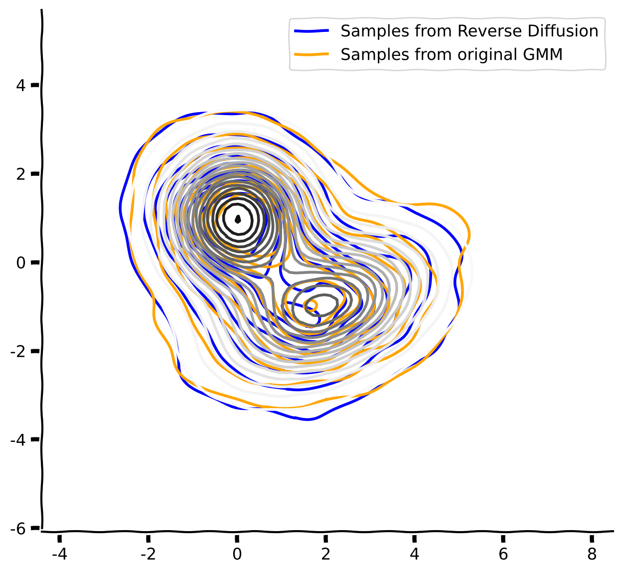
# kdeplot(x0_rev, "Samples from Reverse Diffusion", ax=axs, handles=handles, color="blue")
# kdeplot(gmm_samples, "Samples from original GMM", ax=axs, handles=handles, color="orange")
# gmm_pdf_contour_plot(gmm, cmap="Greys", levels=20)  # the exact pdf contour of gmm
# plt.legend(handles=handles)
# figh.show()

解答を見る$

出力例:

# @title Submit your feedback
content_review(f"{feedback_prefix}_Score_enables_Reversal_of_Diffusion_Exercise")

セクション2: ノイズ除去によるスコアの学習

これまでに、スコア関数が拡散過程の時間反転を可能にすることを理解しました。しかし、分布の解析的な形がない場合、どうやって推定するのでしょうか？

実際のデータセットでは、密度はもちろんスコアにもアクセスできません。しかし、サンプル集合 $\{x_i\}$ はあります。スコアを推定する方法は「ノイズ除去スコアマッチング」と呼ばれます。

上の目的関数（ノイズ除去スコアマッチング、DSM）を最適化することは、下の目的関数（明示的スコアマッチング、ESM）を最適化することと同値であり、これはスコアモデルと真の時間依存スコアの平均二乗誤差（MSE）を最小化します。

J_{DSM}(\theta)=\mathbb E_{x\sim p_0(x)\\\tilde x\sim p_t(\tilde x\mid x)}\|s_\theta(\tilde x)-\nabla_\tilde x\log p_t(\tilde x\mid x)\|^2\\ J_{ESM}(\theta)=\mathbb E_{\tilde x\sim p_t(\tilde x)}\|s_\theta(\tilde x)-\nabla_\tilde x\log p_t(\tilde x)\|^2

どちらの場合も、最適な $s_\theta(x)$ は真のスコア $\nabla_\tilde x\log p_t(\tilde x)$ と同じになります。両者の目的関数は最適解に関して同値です。

順方向過程の条件付き分布 $p_t(\tilde x\mid x)= \mathcal N(x,\sigma^2_t I)$ を利用すると、目的関数はさらに簡単になります。

\mathbb E_{x\sim p_0(x)}\mathbb E_{z\sim \mathcal N(0,I)}\|s_\theta(x+\sigma_t z)+\frac{1}{\sigma_t}z\|^2

すべての $t$ やノイズレベルに対してスコアモデルを学習するために、目的関数は $t\in[\epsilon,1]$ の全時間にわたって積分され、異なる時間に対して重み $\gamma_t$ が付けられます：

\int_\epsilon^1dt \gamma_t\mathbb E_{x\sim p_0(x)}\mathbb E_{z\sim \mathcal N(0,I)}\|s_\theta(x+\sigma_t z, t)+\frac{1}{\sigma_t}z\|^2

ここでは単純な例として、重みを $\gamma_t=\sigma_t^2$ とし、高ノイズ期間( $t\sim 1$ )を低ノイズ期間( $t\sim 0$ )より強調しています：

\int_\epsilon^1dt \mathbb E_{x\sim p_0(x)}\mathbb E_{z\sim \mathcal N(0,I)}\|\sigma_t s_\theta(x+\sigma_t z, t)+z\|^2

平たく言うと、この目的関数は以下の手順を行っています：

訓練分布からクリーンデータ $x$ をサンプリングする $x\sim p_0(x)$
同じ形状の独立同分布ガウスノイズ $z\sim \mathcal N(0,I)$ をサンプリングする
時間 $t$ （またはノイズスケール）をサンプリングし、ノイズ付データ $\tilde x=x+\sigma_t z$ を作成する
ニューラルネットワークで $(\tilde x,t)$ におけるスケールされたノイズを予測し、MSE $\|\sigma_ts_\theta(\tilde x,t)+z\|^2$ を最小化する

拡散モデルは急速に発展している分野で、多様な定式化があります。論文を読むときは怖がらないでください！すべては同じ本質の異なる表現です。

多くの論文（stable diffusionを含む）では、 $-\sigma_t$ をスコアモデルに吸収し、目的関数は $\|\tilde s_\theta(x+\sigma_t z, t)-z\|^2$ の形になり、ノイズをノイズ付サンプルから推定する、つまりノイズ除去の性質を強調します。
- 本ノートブックとコードでは $\|\sigma_t s_\theta(x+\sigma_t z, t)+z\|^2$ の形を使い、スコアの一致を強調しています。
別の種類の順方向過程（分散保存型SDE）では、信号を $\alpha_t$ でスケールダウンしノイズを加えます。その場合、目的関数は $\|\tilde s_\theta(\alpha_t x+\sigma_t z, t)-z\|^2$ の形になります。
最適な重み関数 $\gamma_t$ や切断点 $\epsilon$ はまだ研究が進んでいる分野です。実際の拡散モデルでは多くのヒューリスティックな設定があります。最近の論文を参照してください：

考えてみよう 2: ノイズ除去目的関数

多峰分布のスコアの解釈についての議論を思い出してください。これがノイズ除去目的関数とどう結びつくでしょうか？

原理的には、スコアマッチングの目的関数を0に最適化できますか？なぜでしょう？

2分間静かに考え、その後グループで約10分間議論してください。

解答を見る$

# @title Submit your feedback
content_review(f"{feedback_prefix}_Denoising_objective_Discussion")

コーディング演習 2: ノイズ除去スコアマッチング目的関数の実装

この演習では、DSM目的関数を実装します。

def loss_fn(model, x, sigma_t_fun, eps=1e-5):
  """The loss function for training score-based generative models.

  Args:
    model: A PyTorch model instance that represents a
      time-dependent score-based model.
      it takes x, t as arguments.
    x: A mini-batch of training data.
    sigma_t_fun: A function that gives the standard deviation of the conditional dist.
        p(x_t | x_0)
    eps: A tolerance value for numerical stability, sample t uniformly from [eps, 1.0]
  """
  random_t = torch.rand(x.shape[0], device=x.device) * (1. - eps) + eps
  z = torch.randn_like(x)
  std = sigma_t_fun(random_t, )
  perturbed_x = x + z * std[:, None]
  #################################################
  ## TODO for students: Implement the denoising score matching eq.
  raise NotImplementedError("Student exercise: say what they should have done")
  #################################################
  # use the model to predict score at x_t and t
  score = model(..., ...)
  # implement the loss \|\sigma_t s_\theta(x+\sigma_t z, t) + z\|^2
  loss = ...
  return loss

解答を見る$

正しく実装された損失関数は以下のテストを通過します。

単一の0データ点からなるデータセットでは、解析的スコアは $\mathbf s(\mathbf x,t)=-\mathbf x/\sigma_t^2$ です。この場合、解析的スコアはゼロ損失を持つことをテストします。

# @title Test loss function
sigma_t_test = lambda t: sigma_t(t, Lambda=10)
score_analyt_test = lambda x_t, t: - x_t / sigma_t_test(t)[:, None]**2
x_test = torch.zeros(10, 2)
loss = loss_fn(score_analyt_test, x_test, sigma_t_test, eps=1e-3)
print(f"The loss is zero: {torch.allclose(loss, torch.zeros(1))}")

# @title Submit your feedback
content_review(f"{feedback_prefix}_Implementing_Denoising_Score_Matching_Objective_Exercise")

# @title Define utils functions (Neural Network, and data sampling)
import torch.nn.functional as F
from torch.optim import Adam, SGD
from torch.nn.modules.loss import MSELoss
from tqdm.notebook import trange, tqdm

class GaussianFourierProjection(nn.Module):
  """Gaussian random features for encoding time steps.
  Basically it multiplexes a scalar `t` into a vector of `sin(2 pi k t)` and `cos(2 pi k t)` features.
  """
  def __init__(self, embed_dim, scale=30.):
    super().__init__()
    # Randomly sample weights during initialization. These weights are fixed
    # during optimization and are not trainable.
    self.W = nn.Parameter(torch.randn(embed_dim // 2) * scale, requires_grad=False)
  def forward(self, t):
    t_proj = t[:, None] * self.W[None, :] * 2 * np.pi
    return torch.cat([torch.sin(t_proj), torch.cos(t_proj)], dim=-1)

class ScoreModel_Time(nn.Module):
  """A time-dependent score-based model."""

  def __init__(self, sigma, ):
    super().__init__()
    self.embed = GaussianFourierProjection(10, scale=1)
    self.net = nn.Sequential(nn.Linear(12, 50),
               nn.Tanh(),
               nn.Linear(50,50),
               nn.Tanh(),
               nn.Linear(50,2))
    self.sigma_t_fun = lambda t: np.sqrt(sigma_t_square(t, sigma))

  def forward(self, x, t):
    t_embed = self.embed(t)
    pred = self.net(torch.cat((x,t_embed),dim=1))
    # this additional steps provides an inductive bias.
    # the neural network output on the same scale,
    pred = pred / self.sigma_t_fun(t)[:, None,]
    return pred


def sample_X_and_score_t_depend(gmm, trainN=10000, sigma=5, partition=20, EPS=0.02):
  """Uniformly partition [0,1] and sample t from it, and then
  sample x~ p_t(x) and compute \nabla \log p_t(x)
  finally return the dataset x, score, t (train and test)
  """
  trainN_part = trainN // partition
  X_train_col, y_train_col, T_train_col = [], [], []
  for t in np.linspace(EPS, 1.0, partition):
    gmm_dif = diffuse_gmm(gmm, t, sigma)
    X_train,_,_ = gmm.sample(trainN_part)
    y_train = gmm.score(X_train)
    X_train_tsr = torch.tensor(X_train).float()
    y_train_tsr = torch.tensor(y_train).float()
    T_train_tsr = t * torch.ones(trainN_part)
    X_train_col.append(X_train_tsr)
    y_train_col.append(y_train_tsr)
    T_train_col.append(T_train_tsr)
  X_train_tsr = torch.cat(X_train_col, dim=0)
  y_train_tsr = torch.cat(y_train_col, dim=0)
  T_train_tsr = torch.cat(T_train_col, dim=0)
  return X_train_tsr, y_train_tsr, T_train_tsr

# @title Test the Denoising Score Matching loss function
def test_DSM_objective(gmm, epochs=500, seed=0):
  set_seed(seed)
  sigma = 25.0
  print("sampled 10000 (X, t, score) for training")
  X_train_samp, y_train_samp, T_train_samp = \
    sample_X_and_score_t_depend(gmm, sigma=sigma, trainN=10000,
                              partition=500, EPS=0.01)
  print("sampled 2000 (X, t, score) for testing")
  X_test_samp, y_test_samp, T_test_samp = \
    sample_X_and_score_t_depend(gmm, sigma=sigma, trainN=2000,
                              partition=500, EPS=0.01)
  print("Define neural network score approximator")
  score_model_td = ScoreModel_Time(sigma=sigma)
  sigma_t_f = lambda t: np.sqrt(sigma_t_square(t, sigma))
  optim = Adam(score_model_td.parameters(), lr=0.005)
  print("Minimize the denoising score matching objective")
  stats = []
  pbar = trange(epochs)  # 5k samples for 500 iterations.
  for ep in pbar:
    loss = loss_fn(score_model_td, X_train_samp, sigma_t_f, eps=0.01)
    optim.zero_grad()
    loss.backward()
    optim.step()
    pbar.set_description(f"step {ep} DSM objective loss {loss.item():.3f}")
    if ep % 25==0 or ep==epochs-1:
      # test the score prediction against the analytical score of the gmm.
      y_pred_train = score_model_td(X_train_samp, T_train_samp)
      MSE_train = MSELoss()(y_train_samp, y_pred_train)

      y_pred_test = score_model_td(X_test_samp, T_test_samp)
      MSE_test = MSELoss()(y_test_samp, y_pred_test)
      print(f"step {ep} DSM loss {loss.item():.3f} train score MSE {MSE_train.item():.3f} "+\
          f"test score MSE {MSE_test.item():.3f}")
      stats.append((ep, loss.item(), MSE_train.item(), MSE_test.item()))
  stats_df = pd.DataFrame(stats, columns=['ep', 'DSM_loss', 'MSE_train', 'MSE_test'])
  return score_model_td, stats_df


score_model_td, stats_df = test_DSM_objective(gmm, epochs=500, seed=SEED)

# @title Plot the Loss
stats_df.plot(x="ep", y=['DSM_loss', 'MSE_train', 'MSE_test'])
plt.ylabel("Loss")
plt.xlabel("epoch")
plt.show()

# @title Test the Learned Score by Reverse Diffusion
def reverse_diffusion_SDE_sampling(score_model_td, sampN=500, Lambda=5,
                                   nsteps=200, ndim=2, exact=False):
  """
  score_model_td: if `exact` is True, use a gmm of class GaussianMixture
                  if `exact` is False. use a torch neural network that takes vectorized x and t as input.
  """
  sigmaT2 = sigma_t_square(1, Lambda)
  xT = np.sqrt(sigmaT2) * np.random.randn(sampN, ndim)
  x_traj_rev = np.zeros((*xT.shape, nsteps, ))
  x_traj_rev[:, :, 0] = xT
  dt = 1 / nsteps
  for i in range(1, nsteps):
    t = 1 - i * dt
    tvec = torch.ones((sampN)) * t
    eps_z = np.random.randn(*xT.shape)
    if exact:
      gmm_t = diffuse_gmm(score_model_td, t, Lambda)
      score_xt = gmm_t.score(x_traj_rev[:, :, i-1])
    else:
      with torch.no_grad():
        score_xt = score_model_td(torch.tensor(x_traj_rev[:, :, i-1]).float(), tvec).numpy()
    x_traj_rev[:, :, i] = x_traj_rev[:, :, i-1] + eps_z * (Lambda ** t) * np.sqrt(dt) + score_xt * dt * Lambda**(2*t)
  return x_traj_rev


print("Sample with reverse SDE using the trained score model")
x_traj_rev_appr_denois = reverse_diffusion_SDE_sampling(score_model_td,
                                                        sampN=1000,
                                                        Lambda=25,
                                                        nsteps=200,
                                                        ndim=2)
print("Sample with reverse SDE using the exact score of Gaussian mixture")
x_traj_rev_exact = reverse_diffusion_SDE_sampling(gmm, sampN=1000,
                                                  Lambda=25,
                                                  nsteps=200,
                                                  ndim=2,
                                                  exact=True)
print("Sample from original Gaussian mixture")
X_samp, _, _ = gmm.sample(1000)

print("Compare the distributions")

fig, ax = plt.subplots(figsize=[7, 7])
handles = []
kdeplot(x_traj_rev_appr_denois[:, :, -1],
        label="Reverse diffusion (NN score learned DSM)", handles=handles, color="blue")
kdeplot(x_traj_rev_exact[:, :, -1],
        label="Reverse diffusion (Exact score)", handles=handles, color="orange")
kdeplot(X_samp, label="Samples from original GMM", handles=handles, color="gray")
plt.axis("image")
plt.legend(handles=handles)
plt.show()

まとめ

お疲れさまでした！本日は以下を学びました：

順方向と逆方向の拡散過程がデータ分布とノイズ分布をつなぐ。
サンプリングは逆拡散過程を通じてノイズからデータへの変換を含む。
スコア関数はデータ分布の勾配であり、拡散過程の時間反転を可能にする。
ノイズ除去を学習することで、関数近似器（例：ニューラルネットワーク）を使ってデータのスコア関数を学習できる。

拡散モデルを支える数学は、この確率過程の可逆性です。一般的な結果は、順方向拡散過程が与えられたとき、

d\mathbf{x} = \mathbf{f}(\mathbf{x}, t)dt + g(t)d \mathbf{w}

逆時間の確率過程（逆SDE）が存在し、

d\mathbf{x} = \bigg[\mathbf{f}(\mathbf{x}, t) - g^2(t) \nabla_\mathbf{x} \log p_t(\mathbf{x}) \bigg]dt + g(t) d \mathbf{w}.

確率流常微分方程式（ODE）も存在し、

d\mathbf{x} = \bigg[\mathbf{f}(\mathbf{x}, t) - \frac{1}{2}g^2(t) \nabla_\mathbf{x} \log p_t(\mathbf{x})\bigg] dt.

逆SDEまたは確率流ODEを解くことは、順方向SDEの解の時間反転に相当します。

この数学により、ODEとSDEの両方をシミュレートして拡散モデルからサンプリングできます。

参考文献

ボーナス: スコアマッチング目的関数の数学的背景

サンプルからスコアを推定するにはどうすればよいでしょうか？正確なスコアにアクセスできない場合です。

この目的関数はノイズ除去スコアマッチングと呼ばれ、以下の同値関係$を利用しています。

\begin{align}
$J_{DSM}($ $\theta)$ &= $\mathbb E_{\tilde x,x\sim p_t(\tilde x,x)}$ $\|s_$ $\theta(\tilde x)-\nabla_\tilde x\log p_t(\tilde x\mid x)$ $\|^2\\$
$J_{ESM}($ $\theta)$ &= $\mathbb E_{\tilde x\sim p_t(\tilde x)}$ $\|s_$ $\theta(\tilde x)-\nabla_\tilde x\log p_t(\tilde x)$ $\|^2$
\end{align}

実際には、データ分布から $x$ をサンプリングし、ノイズ $\sigma$ を加えてノイズ除去を行います。時刻 $t$ において、 $p_t(\tilde x\mid x)= \mathcal N(\tilde x;x,\sigma^2_t I)$ なので、 $\tilde x=x+\sigma_t z,z\sim \mathcal N(0,I)$ です。すると

\nabla_\tilde x\log p_t(\tilde x|x)=-\frac{1}{\sigma_t^2}(x+\sigma_t z -x)=-\frac{1}{\sigma_t}z

目的関数は次のように簡略化されます。

\mathbb E_{x\sim p_0(x)}\mathbb E_{z\sim \mathcal N(0,I)} \|s_\theta(x+\sigma_t z)+\frac{1}{\sigma_t}z\|^2

最後に、時間依存スコアモデル $s(x,t)$ では、任意の $t\in [\epsilon,1]$ に対して学習するため、重み関数 $\gamma_t$ を付けて $t$ 全体で積分します。

\int_\epsilon^1dt \gamma_t\mathbb E_{x\sim p_0(x)}\mathbb E_{z\sim \mathcal N(0,I)} \|s_\theta(x+\sigma_t z, t)+\frac{1}{\sigma_t}z\|^2

（ $\epsilon$ は数値安定性のために設定され、 $t\to 0$ で $\sigma_t\to 0$ となるのを防ぎます）
すべての期待値はサンプリングで容易に評価できます。

よく使われる重み付けは次の通りです。

\int_\epsilon^1dt \mathbb E_{x\sim p_0(x)}\mathbb E_{z\sim \mathcal N(0,I)} \|\sigma_t s_\theta(x+\sigma_t z, t)+z\|^2

参考文献

Pascal Vincent (2011), A connection between score matching and denoising autoencoders$