チュートリアル 1: 変分オートエンコーダ（VAE）

第2週、第4日目: 生成モデル

Neuromatch Academyによる

コンテンツ作成者: Saeed Salehi, Spiros Chavlis, Vikash Gilja

コンテンツレビュアー: Diptodip Deb, Kelson Shilling-Scrivo

コンテンツ編集者: Charles J Edelson, Spiros Chavlis

制作編集者: Saeed Salehi, Gagana B, Spiros Chavlis

UPennのコースに触発されて:
講師: Konrad Kording, 元コンテンツ作成者: Richard Lange, Arash Ash

チュートリアルの目標

「生成モデル」日の最初のチュートリアルでは、以下を行います。

教師なし学習／生成モデルについて考え、その有用性を俯瞰的に理解する
潜在変数について直感を養う
オートエンコーダと主成分分析（PCA）の関係を見る
オートエンコーダと変分オートエンコーダを対比しながら、ニューラルネットワークを生成モデルとして考え始める

# @title Tutorial slides
from IPython.display import IFrame
link_id = "rd7ng"
print(f"If you want to download the slides: https://osf.io/download/{link_id}/")
IFrame(src=f"https://mfr.ca-1.osf.io/render?url=https://osf.io/{link_id}/?direct%26mode=render%26action=download%26mode=render", width=854, height=480)

セットアップ

# @title Install dependencies
# @markdown #### Please ignore *errors* and/or *warnings* during installation.

# @title Install and import feedback gadget


from vibecheck import DatatopsContentReviewContainer
def content_review(notebook_section: str):
    return DatatopsContentReviewContainer(
        "",  # No text prompt
        notebook_section,
        {
            "url": "https://pmyvdlilci.execute-api.us-east-1.amazonaws.com/klab",
            "name": "neuromatch_dl",
            "user_key": "f379rz8y",
        },
    ).render()


feedback_prefix = "W2D4_T1"

# Imports
import torch
import random

import numpy as np
import matplotlib.pylab as plt

import torch.nn as nn
import torch.nn.functional as F
from torch.utils.data import DataLoader

import torchvision
from torchvision import datasets, transforms

from pytorch_pretrained_biggan import one_hot_from_names

from tqdm.notebook import tqdm, trange

# @title Figure settings
import logging
logging.getLogger('matplotlib.font_manager').disabled = True

import ipywidgets as widgets
from ipywidgets import FloatSlider, IntSlider, HBox, Layout, VBox
from ipywidgets import interactive_output, Dropdown

%config InlineBackend.figure_format = 'retina'
plt.style.use("https://raw.githubusercontent.com/NeuromatchAcademy/content-creation/main/nma.mplstyle")

# @title Helper functions


def image_moments(image_batches, n_batches=None):
  """
  Compute mean and covariance of all pixels
  from batches of images

  Args:
    Image_batches: tuple
      Image batches
    n_batches: int
      Number of Batch size

  Returns:
    m1: float
      Mean of all pixels
    cov: float
      Covariance of all pixels
  """
  m1, m2 = torch.zeros((), device=DEVICE), torch.zeros((), device=DEVICE)
  n = 0
  for im in tqdm(image_batches, total=n_batches, leave=False,
                 desc='Computing pixel mean and covariance...'):
    im = im.to(DEVICE)
    b = im.size()[0]
    im = im.view(b, -1)
    m1 = m1 + im.sum(dim=0)
    m2 = m2 + (im.view(b,-1,1) * im.view(b,1,-1)).sum(dim=0)
    n += b
  m1, m2 = m1/n, m2/n
  cov = m2 - m1.view(-1,1)*m1.view(1,-1)
  return m1.cpu(), cov.cpu()


def interpolate(A, B, num_interps):
  """
  Function to interpolate between images.
  It does this by linearly interpolating between the
  probability of each category you select and linearly
  interpolating between the latent vector values.

  Args:
    A: list
      List of categories
    B: list
      List of categories
    num_interps: int
      Quantity of pixel grids

  Returns:
    Interpolated np.ndarray
  """
  if A.shape != B.shape:
    raise ValueError('A and B must have the same shape to interpolate.')
  alphas = np.linspace(0, 1, num_interps)
  return np.array([(1-a)*A + a*B for a in alphas])


def kl_q_p(zs, phi):
  """
  Given [b,n,k] samples of z drawn
  from q, compute estimate of KL(q||p).
  phi must be size [b,k+1]
  This uses mu_p = 0 and sigma_p = 1,
  which simplifies the log(p(zs)) term to
  just -1/2*(zs**2)

  Args:
    zs: list
      Samples
    phi: list
      Relative entropy

  Returns:
    Size of log_q and log_p is [b,n,k].
    Sum along [k] but mean along [b,n]
  """
  b, n, k = zs.size()
  mu_q, log_sig_q = phi[:,:-1], phi[:,-1]
  log_p = -0.5*(zs**2)
  log_q = -0.5*(zs - mu_q.view(b,1,k))**2 / log_sig_q.exp().view(b,1,1)**2 - log_sig_q.view(b,1,-1)
  # Size of log_q and log_p is [b,n,k].
  # Sum along [k] but mean along [b,n]
  return (log_q - log_p).sum(dim=2).mean(dim=(0,1))


def log_p_x(x, mu_xs, sig_x):
  """
  Given [batch, ...] input x and
  [batch, n, ...] reconstructions, compute
  pixel-wise log Gaussian probability
  Sum over pixel dimensions, but mean over batch
  and samples.

  Args:
    x: np.ndarray
      Input Data
    mu_xs: np.ndarray
      Log of mean of samples
    sig_x: np.ndarray
      Log of standard deviation

  Returns:
    Mean over batch and samples.
  """
  b, n = mu_xs.size()[:2]
  # Flatten out pixels and add a singleton
  # dimension [1] so that x will be
  # implicitly expanded when combined with mu_xs
  x = x.reshape(b, 1, -1)
  _, _, p = x.size()
  squared_error = (x - mu_xs.view(b, n, -1))**2 / (2*sig_x**2)

  # Size of squared_error is [b,n,p]. log prob is
  # by definition sum over [p].
  # Expected value requires mean over [n].
  # Handling different size batches
  # requires mean over [b].
  return -(squared_error + torch.log(sig_x)).sum(dim=2).mean(dim=(0,1))


def pca_encoder_decoder(mu, cov, k):
  """
  Compute encoder and decoder matrices
  for PCA dimensionality reduction

  Args:
    mu: np.ndarray
      Mean
    cov: float
      Covariance
    k: int
      Dimensionality

  Returns:
    Nothing
  """
  mu = mu.view(1,-1)
  u, s, v = torch.svd_lowrank(cov, q=k)
  W_encode = v / torch.sqrt(s)
  W_decode = u * torch.sqrt(s)

  def pca_encode(x):
    """
    Encoder: Subtract mean image and
    project onto top K eigenvectors of
    the data covariance

    Args:
      x: torch.tensor
        Input data

    Returns:
      PCA Encoding
    """
    return (x.view(-1,mu.numel()) - mu) @ W_encode

  def pca_decode(h):
    """
    Decoder: un-project then add back in the mean

    Args:
      h: torch.tensor
        Hidden layer data

    Returns:
      PCA Decoding
    """
    return (h @ W_decode.T) + mu

  return pca_encode, pca_decode


def cout(x, layer):
  """
  Unnecessarily complicated but complete way to
  calculate the output depth, height
  and width size for a Conv2D layer

  Args:
    x: tuple
      Input size (depth, height, width)
    layer: nn.Conv2d
      The Conv2D layer

  Returns:
    Tuple of out-depth/out-height and out-width
    Output shape as given in [Ref]
    Ref:
    https://pytorch.org/docs/stable/generated/torch.nn.Conv2d.html
  """
  assert isinstance(layer, nn.Conv2d)
  p = layer.padding if isinstance(layer.padding, tuple) else (layer.padding,)
  k = layer.kernel_size if isinstance(layer.kernel_size, tuple) else (layer.kernel_size,)
  d = layer.dilation if isinstance(layer.dilation, tuple) else (layer.dilation,)
  s = layer.stride if isinstance(layer.stride, tuple) else (layer.stride,)
  in_depth, in_height, in_width = x
  out_depth = layer.out_channels
  out_height = 1 + (in_height + 2 * p[0] - (k[0] - 1) * d[0] - 1) // s[0]
  out_width = 1 + (in_width + 2 * p[-1] - (k[-1] - 1) * d[-1] - 1) // s[-1]
  return (out_depth, out_height, out_width)

# @title Plotting functions

def plot_gen_samples_ppca(therm1, therm2, therm_data_sim):
  """
  Plotting generated samples

  Args:
    therm1: list
      Thermometer 1
    them2: list
      Thermometer 2
    therm_data_sim: list
      Generated (simulate, draw) `n_samples` from pPCA model

  Returns:
    Nothing
  """
  plt.plot(therm1, therm2, '.', c='c', label='training data')
  plt.plot(therm_data_sim[0], therm_data_sim[1], '.', c='m', label='"generated" data')
  plt.axis('equal')
  plt.xlabel('Thermometer 1 ($^\circ$C)')
  plt.ylabel('Thermometer 2 ($^\circ$C)')
  plt.legend()
  plt.show()


def plot_linear_ae(lin_losses):
  """
  Plotting linear autoencoder

  Args:
    lin_losses: list
      Log of linear autoencoder MSE losses

  Returns:
    Nothing
  """
  plt.figure()
  plt.plot(lin_losses)
  plt.ylim([0, 2*torch.as_tensor(lin_losses).median()])
  plt.xlabel('Training batch')
  plt.ylabel('MSE Loss')
  plt.show()


def plot_conv_ae(lin_losses, conv_losses):
  """
  Plotting convolutional autoencoder

  Args:
    lin_losses: list
      Log of linear autoencoder MSE losses
    conv_losses: list
      Log of convolutional model MSe losses

  Returns:
    Nothing
  """
  plt.figure()
  plt.plot(lin_losses)
  plt.plot(conv_losses)
  plt.legend(['Lin AE', 'Conv AE'])
  plt.xlabel('Training batch')
  plt.ylabel('MSE Loss')
  plt.ylim([0,
            2*max(torch.as_tensor(conv_losses).median(),
                  torch.as_tensor(lin_losses).median())])
  plt.show()


def plot_images(images, h=3, w=3, plt_title=''):
  """
  Helper function to plot images

  Args:
    images: torch.tensor
      Images
    h: int
      Image height
    w: int
      Image width
    plt_title: string
      Plot title

  Returns:
    Nothing
  """
  plt.figure(figsize=(h*2, w*2))
  plt.suptitle(plt_title, y=1.03)
  for i in range(h*w):
    plt.subplot(h, w, i + 1)
    plot_torch_image(images[i])
  plt.axis('off')
  plt.show()

def plot_phi(phi, num=4):
  """
  Contour plot of relative entropy across samples

  Args:
    phi: list
      Log of relative entropu changes
    num: int
      Number of interations
  """
  plt.figure(figsize=(12, 3))
  for i in range(num):
    plt.subplot(1, num, i + 1)
    plt.scatter(zs[i, :, 0], zs[i, :, 1], marker='.')
    th = torch.linspace(0, 6.28318, 100)
    x, y = torch.cos(th), torch.sin(th)
    # Draw 2-sigma contours
    plt.plot(
        2*x*phi[i, 2].exp().item() + phi[i, 0].item(),
        2*y*phi[i, 2].exp().item() + phi[i, 1].item()
        )
    plt.xlim(-5, 5)
    plt.ylim(-5, 5)
    plt.grid()
    plt.axis('equal')
  plt.suptitle('If rsample() is correct, then most but not all points should lie in the circles')
  plt.show()


def plot_torch_image(image, ax=None):
  """
  Helper function to plot torch image

  Args:
    image: torch.tensor
      Image
    ax: plt object
      If None, plt.gca()

  Returns:
    Nothing
  """
  ax = ax if ax is not None else plt.gca()
  c, h, w = image.size()
  if c==1:
    cm = 'gray'
  else:
    cm = None

  # Torch images have shape (channels, height, width)
  # but matplotlib expects
  # (height, width, channels) or just
  # (height,width) when grayscale
  im_plt = torch.clip(image.detach().cpu().permute(1,2,0).squeeze(), 0.0, 1.0)
  ax.imshow(im_plt, cmap=cm)
  ax.set_xticks([])
  ax.set_yticks([])
  ax.spines['right'].set_visible(False)
  ax.spines['top'].set_visible(False)

# @title Set random seed

# @markdown Executing `set_seed(seed=seed)` you are setting the seed

# For DL its critical to set the random seed so that students can have a
# baseline to compare their results to expected results.
# Read more here: https://pytorch.org/docs/stable/notes/randomness.html

# Call `set_seed` function in the exercises to ensure reproducibility.
import random
import torch

def set_seed(seed=None, seed_torch=True):
  """
  Function that controls randomness. NumPy and random modules must be imported.

  Args:
    seed : Integer
      A non-negative integer that defines the random state. Default is `None`.
    seed_torch : Boolean
      If `True` sets the random seed for pytorch tensors, so pytorch module
      must be imported. Default is `True`.

  Returns:
    Nothing.
  """
  if seed is None:
    seed = np.random.choice(2 ** 32)
  random.seed(seed)
  np.random.seed(seed)
  if seed_torch:
    torch.manual_seed(seed)
    torch.cuda.manual_seed_all(seed)
    torch.cuda.manual_seed(seed)
    torch.backends.cudnn.benchmark = False
    torch.backends.cudnn.deterministic = True

  print(f'Random seed {seed} has been set.')


# In case that `DataLoader` is used
def seed_worker(worker_id):
  """
  DataLoader will reseed workers following randomness in
  multi-process data loading algorithm.

  Args:
    worker_id: integer
      ID of subprocess to seed. 0 means that
      the data will be loaded in the main process
      Refer: https://pytorch.org/docs/stable/data.html#data-loading-randomness for more details

  Returns:
    Nothing
  """
  worker_seed = torch.initial_seed() % 2**32
  np.random.seed(worker_seed)
  random.seed(worker_seed)

# @title Set device (GPU or CPU). Execute `set_device()`
# especially if torch modules used.

# Inform the user if the notebook uses GPU or CPU.

def set_device():
  """
  Set the device. CUDA if available, CPU otherwise

  Args:
    None

  Returns:
    Nothing
  """
  device = "cuda" if torch.cuda.is_available() else "cpu"
  if device != "cuda":
    print("WARNING: For this notebook to perform best, "
        "if possible, in the menu under `Runtime` -> "
        "`Change runtime type.`  select `GPU` ")
  else:
    print("GPU is enabled in this notebook.")

  return device

SEED = 2021
set_seed(seed=SEED)
DEVICE = set_device()

# @title Download `wordnet` dataset

"""
NLTK Download:

import nltk
nltk.download('wordnet')
"""

import os, requests, zipfile

os.environ['NLTK_DATA'] = 'nltk_data/'

fnames = ['wordnet.zip', 'omw-1.4.zip']
urls = ['https://osf.io/ekjxy/download', 'https://osf.io/kuwep/download']

for fname, url in zip(fnames, urls):
  r = requests.get(url, allow_redirects=True)

  with open(fname, 'wb') as fd:
    fd.write(r.content)

  with zipfile.ZipFile(fname, 'r') as zip_ref:
    zip_ref.extractall('nltk_data/corpora')

セクション 1: 生成モデル

所要時間の目安: 約15分

動画の後にセルを実行して、BigGAN（生成モデル）といくつかの標準的な画像データセットを動画再生中にダウンロードしてください。

# @title Video 1: Generative Modeling
from ipywidgets import widgets
from IPython.display import YouTubeVideo
from IPython.display import IFrame
from IPython.display import display


class PlayVideo(IFrame):
  def __init__(self, id, source, page=1, width=400, height=300, **kwargs):
    self.id = id
    if source == 'Bilibili':
      src = f'https://player.bilibili.com/player.html?bvid={id}&page={page}'
    elif source == 'Osf':
      src = f'https://mfr.ca-1.osf.io/render?url=https://osf.io/download/{id}/?direct%26mode=render'
    super(PlayVideo, self).__init__(src, width, height, **kwargs)


def display_videos(video_ids, W=400, H=300, fs=1):
  tab_contents = []
  for i, video_id in enumerate(video_ids):
    out = widgets.Output()
    with out:
      if video_ids[i][0] == 'Youtube':
        video = YouTubeVideo(id=video_ids[i][1], width=W,
                             height=H, fs=fs, rel=0)
        print(f'Video available at https://youtube.com/watch?v={video.id}')
      else:
        video = PlayVideo(id=video_ids[i][1], source=video_ids[i][0], width=W,
                          height=H, fs=fs, autoplay=False)
        if video_ids[i][0] == 'Bilibili':
          print(f'Video available at https://www.bilibili.com/video/{video.id}')
        elif video_ids[i][0] == 'Osf':
          print(f'Video available at https://osf.io/{video.id}')
      display(video)
    tab_contents.append(out)
  return tab_contents


video_ids = [('Youtube', '5EEx0sdyR_U'), ('Bilibili', 'BV1Vy4y1j7cN')]
tab_contents = display_videos(video_ids, W=854, H=480)
tabs = widgets.Tab()
tabs.children = tab_contents
for i in range(len(tab_contents)):
  tabs.set_title(i, video_ids[i][0])
display(tabs)

# @title Submit your feedback
content_review(f"{feedback_prefix}_Generative_Modeling_Video")

# @markdown Download BigGAN (a generative model) and a few standard image datasets

## Initially was downloaded directly
# biggan_model = BigGAN.from_pretrained('biggan-deep-256')

url = "https://osf.io/3yvhw/download"
fname = "biggan_deep_256"
r = requests.get(url, allow_redirects=True)
with open(fname, 'wb') as fd:
  fd.write(r.content)

biggan_model = torch.load(fname)

セクション 1.1: BigGANからの画像生成

生成モデルの力を示すために、完全に訓練された生成モデルであるBigGANの先行体験を提供します。今日の後半で（より多くの背景知識を得た上で）再度登場します。今は、BigGANを生成モデルとして見ることに集中しましょう。具体的には、BigGANは $128 \times 128$ 画像のクラス条件付き生成モデルです。クラスは画像を説明するカテゴリラベルに基づいており、画像はベクトル（動画講義での $z$ ）と特定の離散カテゴリに属する確率に基づいて生成されます。

今は、ベクトルとカテゴリラベルに基づいて画像を生成するという点以外のモデルの詳細は気にしなくて構いません。

インタラクティブデモ 1.1: BigGANジェネレーター

生成された画像の空間を探索するために、カテゴリラベルを選択し、4つの異なるzベクトルを生成し、それらのzベクトルに基づく生成画像を表示できるウィジェットを用意しました。zベクトルは128次元で、一見高次元に思えますが、 $128 \times 128$ 画像よりはるかに低次元です！

さらに下にスライダーオプションが1つあります：zベクトルは切断正規分布から生成されており、切断値を選択できます。基本的に、ベクトルの大きさを制御していることになります。今は詳細を気にする必要はありません。ここでは概念的なポイントを示しているだけで、切断値やzベクトルの細かい仕組みを知る必要はありません。

カテゴリや切断値スライダーを変更するたびに、4つの異なるzベクトルが生成され、それに対応する4つの異なる画像が得られます。

# @markdown BigGAN Image Generator (the updates may take a few seconds, please be patient)

# category = 'German shepherd' # @param ['tench', 'magpie', 'jellyfish', 'German shepherd', 'bee', 'acoustic guitar', 'coffee mug', 'minibus', 'monitor']
# z_magnitude = .1 # @param {type:"slider", min:0, max:1, step:.1}


from scipy.stats import truncnorm
def truncated_noise_sample(batch_size=1, dim_z=128, truncation=1., seed=None):
    """ Create a truncated noise vector.
        Params:
            batch_size: batch size.
            dim_z: dimension of z
            truncation: truncation value to use
            seed: seed for the random generator
        Output:
            array of shape (batch_size, dim_z)
    """
    state = None if seed is None else np.random.RandomState(seed)
    values = truncnorm.rvs(-2, 2, size=(batch_size, dim_z), random_state=state).astype(np.float32)
    return truncation * values


def sample_from_biggan(category, z_magnitude):
  """
  Sample from BigGAN Image Generator

  Args:
    category: string
      Category
    z_magnitude: int
      Magnitude of variation vector

  Returns:
    Nothing
  """

  truncation = z_magnitude
  z = truncated_noise_sample(truncation=truncation, batch_size=4)
  y = one_hot_from_names(category, batch_size=4)

  z = torch.from_numpy(z)
  z = z.float()
  y = torch.from_numpy(y)

  # Move to GPU
  z = z.to(device=set_device())
  y = y.to(device=set_device())
  biggan_model.to(device=set_device())


  with torch.no_grad():
    output = biggan_model(z, y, truncation)

  # Back to CPU
  output = output.to('cpu')

  # The output layer of BigGAN has a tanh layer,
  # resulting the range of [-1, 1] for the output image
  # Therefore, we normalize the images properly to [0, 1]
  # range.
  # Clipping is only in case of numerical instability
  # problems

  output = torch.clip(((output.detach().clone() + 1) / 2.0), 0, 1)

  fig, axes = plt.subplots(2, 2)
  axes = axes.flatten()
  for im in range(4):

    axes[im].imshow(output[im].squeeze().moveaxis(0,-1))
    axes[im].axis('off')

z_slider = FloatSlider(min=.1, max=1, step=.1, value=0.1,
                     continuous_update=False,
                     description='Truncation Value',
                     style = {'description_width': '100px'},
                     layout=Layout(width='440px'))

category_dropdown = Dropdown(
    options=['tench', 'magpie', 'jellyfish', 'German shepherd', 'bee',
             'acoustic guitar', 'coffee mug', 'minibus', 'monitor'],
             value="German shepherd",
             description="Category: ")

widgets_ui = VBox([category_dropdown, z_slider])

widgets_out = interactive_output(sample_from_biggan,
                                 {
                                  'z_magnitude': z_slider,
                                  'category': category_dropdown
                                  }
                                 )

display(widgets_ui, widgets_out)

考えてみよう！1.1: 生成された画像

生成された画像はどのように見えますか？リアルに見えますか、それとも明らかに偽物に見えますか？

切断値を上げると、生成画像やそれらの関係性についてどのような変化が見られますか？

解答を見る$

# @title Submit your feedback
content_review(f"{feedback_prefix}_Generated_Images_Discussion")

セクション 1.2: BigGANによる画像の補間

次のウィジェットでは、2つの生成画像の間を補間できます。これは、選択した各カテゴリの確率を線形補間し、潜在ベクトルの値も線形補間することで実現しています。

インタラクティブデモ 1.2: BigGAN補間

# @markdown BigGAN Interpolation Widget (the updates may take a few seconds)

def interpolate_biggan(category_A,
                       category_B):
  """
  Interpolation function with BigGan

  Args:
    category_A: string
      Category specification
    category_B: string
      Category specification

  Returns:
    Nothing
  """
  num_interps = 16

  # category_A = 'jellyfish' #@param ['tench', 'magpie', 'jellyfish', 'German shepherd', 'bee', 'acoustic guitar', 'coffee mug', 'minibus', 'monitor']
  # z_magnitude_A = 0 #@param {type:"slider", min:-10, max:10, step:1}

  # category_B = 'German shepherd' #@param ['tench', 'magpie', 'jellyfish', 'German shepherd', 'bee', 'acoustic guitar', 'coffee mug', 'minibus', 'monitor']
  # z_magnitude_B = 0 #@param {type:"slider", min:-10, max:10, step:1}


  def interpolate_and_shape(A, B, num_interps):
    """
    Function to interpolate and shape images.
    It does this by linearly interpolating between the
    probability of each category you select and linearly
    interpolating between the latent vector values.

    Args:
      A: list
        List of categories
      B: list
        List of categories
      num_interps: int
        Quantity of pixel grids

    Returns:
      Interpolated np.ndarray
    """
    interps = interpolate(A, B, num_interps)
    return (interps.transpose(1, 0, *range(2, len(interps.shape))).reshape(num_interps, *interps.shape[2:]))

  # unit_vector = np.ones((1, 128))/np.sqrt(128)
  # z_A = z_magnitude_A * unit_vector
  # z_B = z_magnitude_B * unit_vector
  truncation = .4
  z_A = truncated_noise_sample(truncation=truncation, batch_size=1)
  z_B = truncated_noise_sample(truncation=truncation, batch_size=1)
  y_A = one_hot_from_names(category_A, batch_size=1)
  y_B = one_hot_from_names(category_B, batch_size=1)

  z_interp = interpolate_and_shape(z_A, z_B, num_interps)
  y_interp = interpolate_and_shape(y_A, y_B, num_interps)

  # Convert to tensor
  z_interp = torch.from_numpy(z_interp)
  z_interp = z_interp.float()
  y_interp = torch.from_numpy(y_interp)

  # Move to GPU
  z_interp = z_interp.to(DEVICE)
  y_interp = y_interp.to(DEVICE)
  biggan_model.to(DEVICE)

  with torch.no_grad():
    output = biggan_model(z_interp, y_interp, 1)

  # Back to CPU
  output = output.to('cpu')

  # The output layer of BigGAN has a tanh layer,
  # resulting the range of [-1, 1] for the output image
  # Therefore, we normalize the images properly to
  # [0, 1] range.
  # Clipping is only in case of numerical instability
  # problems

  output = torch.clip(((output.detach().clone() + 1) / 2.0), 0, 1)
  output = output

  # Make grid and show generated samples
  output_grid = torchvision.utils.make_grid(output,
                                            nrow=min(4, output.shape[0]),
                                            padding=5)
  plt.axis('off');
  plt.imshow(output_grid.permute(1, 2, 0))
  plt.show()


# z_A_slider = IntSlider(min=-10, max=10, step=1, value=0,
#                        continuous_update=False, description='Z Magnitude A',
#                        layout=Layout(width='440px'),
#                        style={'description_width': 'initial'})

# z_B_slider = IntSlider(min=-10, max=10, step=1, value=0,
#                        continuous_update=False, description='Z Magntude B',
#                        layout=Layout(width='440px'),
#                        style={'description_width': 'initial'})

category_A_dropdown = Dropdown(
    options=['tench', 'magpie', 'jellyfish', 'German shepherd', 'bee',
             'acoustic guitar', 'coffee mug', 'minibus', 'monitor'],
             value="German shepherd",
             description="Category A: ")

category_B_dropdown = Dropdown(
    options=['tench', 'magpie', 'jellyfish', 'German shepherd', 'bee',
             'acoustic guitar', 'coffee mug', 'minibus', 'monitor'],
             value="jellyfish",
             description="Category B: ")



widgets_ui = VBox([HBox([category_A_dropdown]),
                   HBox([category_B_dropdown])])

widgets_out = interactive_output(interpolate_biggan,
                                 {'category_A': category_A_dropdown,
                                  # 'z_magnitude_A': z_A_slider,
                                  'category_B': category_B_dropdown})
                                  # 'z_magnitude_B': z_B_slider})

display(widgets_ui, widgets_out)

# @title Submit your feedback
content_review(f"{feedback_prefix}_BigGAN_Interpolation_Interactive_Demo")

考えてみよう！1.2: 同じカテゴリのサンプル間の補間

同じカテゴリのサンプル間、類似したカテゴリのサンプル間、非常に異なるカテゴリのサンプル間で補間を試してみてください。何か傾向に気づきますか？これは潜在空間における画像の表現について何を示唆しているでしょうか？

解答を見る$

# @title Submit your feedback
content_review(f"{feedback_prefix}_Samples_from_the_same_category_Discussion")

セクション 2: 潜在変数モデル

所要時間の目安: ボーナスを除いて約15分

# @title Video 2: Latent Variable Models
from ipywidgets import widgets
from IPython.display import YouTubeVideo
from IPython.display import IFrame
from IPython.display import display


class PlayVideo(IFrame):
  def __init__(self, id, source, page=1, width=400, height=300, **kwargs):
    self.id = id
    if source == 'Bilibili':
      src = f'https://player.bilibili.com/player.html?bvid={id}&page={page}'
    elif source == 'Osf':
      src = f'https://mfr.ca-1.osf.io/render?url=https://osf.io/download/{id}/?direct%26mode=render'
    super(PlayVideo, self).__init__(src, width, height, **kwargs)


def display_videos(video_ids, W=400, H=300, fs=1):
  tab_contents = []
  for i, video_id in enumerate(video_ids):
    out = widgets.Output()
    with out:
      if video_ids[i][0] == 'Youtube':
        video = YouTubeVideo(id=video_ids[i][1], width=W,
                             height=H, fs=fs, rel=0)
        print(f'Video available at https://youtube.com/watch?v={video.id}')
      else:
        video = PlayVideo(id=video_ids[i][1], source=video_ids[i][0], width=W,
                          height=H, fs=fs, autoplay=False)
        if video_ids[i][0] == 'Bilibili':
          print(f'Video available at https://www.bilibili.com/video/{video.id}')
        elif video_ids[i][0] == 'Osf':
          print(f'Video available at https://osf.io/{video.id}')
      display(video)
    tab_contents.append(out)
  return tab_contents


video_ids = [('Youtube', '_e0nKUeBDFo'), ('Bilibili', 'BV1Db4y167Ys')]
tab_contents = display_videos(video_ids, W=854, H=480)
tabs = widgets.Tab()
tabs.children = tab_contents
for i in range(len(tab_contents)):
  tabs.set_title(i, video_ids[i][0])
display(tabs)

# @title Submit your feedback
content_review(f"{feedback_prefix}_Latent_Variable_Models_Video")

動画では潜在変数モデルの概念が紹介されました。PCA（主成分分析）が潜在変数を持つ生成モデル、すなわち確率的PCA（pPCA）に拡張できることを見ました。pPCAにおいて潜在変数（動画中のz）は主成分軸への射影です。

主成分の次元数は通常、元のデータよりもかなり低次元に設定されます。したがって、潜在変数（主成分軸への射影）は元のデータの低次元表現（次元削減！）となります。pPCAを用いることで高次元データの元の分布を推定できます。これにより、単にPCAで潜在変数からデータを生成するよりも、元のデータに「より似た」分布のデータを生成できます。簡単な例で見てみましょう。

（ボーナス）コーディング演習 2: pPCA

同じ部屋の温度を測る2つのノイズのある温度計があるとします。両方ともノイズのある測定をします。部屋の温度はおよそ25℃（77°F）前後で変動します。時間をかけて2つの温度計から多くの測定値を取り、そのペアの測定値をプロットすると、以下のような図になるかもしれません。

# @markdown Generate example datapoints from the two thermometers

def generate_data(n_samples, mean_of_temps, cov_of_temps, seed):
  """
  Generate random data, normally distributed

  Args:
    n_samples : int
      The number of samples to be generated
    mean_of_temps : numpy.ndarray
      1D array with the mean of temparatures, Kx1
    cov_of_temps : numpy.ndarray
      2D array with the covariance, , KxK
    seed : int
      Set random seed for the psudo random generator

  Returns:
    therm1 : numpy.ndarray
      Thermometer 1
    therm2 : numpy.ndarray
      Thermometer 2
  """

  np.random.seed(seed)
  therm1, therm2 = np.random.multivariate_normal(mean_of_temps,
                                                cov_of_temps,
                                                n_samples).T
  return therm1, therm2


n_samples = 2000
mean_of_temps = np.array([25, 25])
cov_of_temps = np.array([[10, 5], [5, 10]])
therm1, therm2 = generate_data(n_samples, mean_of_temps, cov_of_temps, seed=SEED)

plt.plot(therm1, therm2, '.')
plt.axis('equal')
plt.xlabel('Thermometer 1 ($^\circ$C)')
plt.ylabel('Thermometer 2 ($^\circ$C)')
plt.show()

これらのデータを単一の主成分でモデル化しましょう。温度計は同じ実際の温度を測っているため、主成分軸は単位線（恒等線）になります。この軸の方向は単位ベクトル $[1 ~~ 1]~/~\sqrt2$ で示されます。PCAを適用してこの軸を推定できます。この軸をプロットするとデータの特徴がわかりますが、これだけでは生成はできません。

# @markdown Add first PC axes to the plot

plt.plot(therm1, therm2, '.')
plt.axis('equal')
plt.xlabel('Thermometer 1 ($^\circ$C)')
plt.ylabel('Thermometer 2 ($^\circ$C)')
plt.plot([plt.axis()[0], plt.axis()[1]],
         [plt.axis()[0], plt.axis()[1]])
plt.show()

ステップ 1: pPCAモデルのパラメータを計算する

この部分はすでに完成しているので、編集は不要です。

# Project Data onto the principal component axes.
# We could have "learned" this from the data by applying PCA,
# but we "know" the value from the problem definition.
pc_axes = np.array([1.0, 1.0]) / np.sqrt(2.0)

# Thermometers data
therm_data = np.array([therm1, therm2])

# Zero center the data
therm_data_mean = np.mean(therm_data, 1)
therm_data_center = np.outer(therm_data_mean, np.ones(therm_data.shape[1]))
therm_data_zero_centered = therm_data - therm_data_center

# Calculate the variance of the projection on the PC axes
pc_projection = np.matmul(pc_axes, therm_data_zero_centered);
pc_axes_variance = np.var(pc_projection)

# Calculate the residual variance (variance not accounted for by projection on the PC axes)
sensor_noise_std = np.mean(np.linalg.norm(therm_data_zero_centered - np.outer(pc_axes, pc_projection), axis=0, ord=2))
sensor_noise_var = sensor_noise_std **2

ステップ 2: 温度計データのpPCAモデルから「生成」する。

pPCAモデルに従ってサンプリングし、データを生成するコードを完成させてください：

x = \mu + W z + \epsilon, \,\text{ここで}\,~~ \epsilon \sim \mathcal{N}(0,~\sigma^2 \mathbf{I})

def gen_from_pPCA(noise_var, data_mean, pc_axes, pc_variance):
  """
  Generate samples from pPCA

  Args:
    noise_var: np.ndarray
      Sensor noise variance
    data_mean: np.ndarray
      Thermometer data mean
    pc_axes: np.ndarray
      Principal component axes
    pc_variance: np.ndarray
      The variance of the projection on the PC axes

  Returns:
    therm_data_sim: np.ndarray
      Generated (simulate, draw) `n_samples` from pPCA model
  """
  # We are matching this value to the thermometer data so the visualizations look similar
  n_samples = 1000

  # Randomly sample from z (latent space value)
  z = np.random.normal(0.0, np.sqrt(pc_variance), n_samples)

  # Sensor noise covariance matrix (∑)
  epsilon_cov = [[noise_var, 0.0], [0.0, noise_var]]

  # Data mean reshaped for the generation
  sim_mean = np.outer(data_mean, np.ones(n_samples))

  ####################################################################
  # Fill in all missing code below (...),
  # then remove or comment the line below to test your class
  raise NotImplementedError("Please complete the `gen_from_pPCA` function")
  ####################################################################
  # Draw `n_samples` from `np.random.multivariate_normal`
  rand_eps = ...
  rand_eps = rand_eps.T

  # Generate (simulate, draw) `n_samples` from pPCA model
  therm_data_sim = ...

  return therm_data_sim



## Uncomment to test your code
# therm_data_sim = gen_from_pPCA(sensor_noise_var, therm_data_mean, pc_axes, pc_axes_variance)
# plot_gen_samples_ppca(therm1, therm2, therm_data_sim)

解答を見る$

# @title Submit your feedback
content_review(f"{feedback_prefix}_Coding_pPCA_Exercise")

セクション 3: オートエンコーダー

所要時間の目安: 約30分

動画を見ながら、動画の後にあるセルを実行してMNISTとCIFAR10の画像データセットをダウンロードしてください。

# @title Video 3: Autoencoders
from ipywidgets import widgets
from IPython.display import YouTubeVideo
from IPython.display import IFrame
from IPython.display import display


class PlayVideo(IFrame):
  def __init__(self, id, source, page=1, width=400, height=300, **kwargs):
    self.id = id
    if source == 'Bilibili':
      src = f'https://player.bilibili.com/player.html?bvid={id}&page={page}'
    elif source == 'Osf':
      src = f'https://mfr.ca-1.osf.io/render?url=https://osf.io/download/{id}/?direct%26mode=render'
    super(PlayVideo, self).__init__(src, width, height, **kwargs)


def display_videos(video_ids, W=400, H=300, fs=1):
  tab_contents = []
  for i, video_id in enumerate(video_ids):
    out = widgets.Output()
    with out:
      if video_ids[i][0] == 'Youtube':
        video = YouTubeVideo(id=video_ids[i][1], width=W,
                             height=H, fs=fs, rel=0)
        print(f'Video available at https://youtube.com/watch?v={video.id}')
      else:
        video = PlayVideo(id=video_ids[i][1], source=video_ids[i][0], width=W,
                          height=H, fs=fs, autoplay=False)
        if video_ids[i][0] == 'Bilibili':
          print(f'Video available at https://www.bilibili.com/video/{video.id}')
        elif video_ids[i][0] == 'Osf':
          print(f'Video available at https://osf.io/{video.id}')
      display(video)
    tab_contents.append(out)
  return tab_contents


video_ids = [('Youtube', 'MlyIL1PmDCA'), ('Bilibili', 'BV16b4y167Z2')]
tab_contents = display_videos(video_ids, W=854, H=480)
tabs = widgets.Tab()
tabs.children = tab_contents
for i in range(len(tab_contents)):
  tabs.set_title(i, video_ids[i][0])
display(tabs)

# @title Submit your feedback
content_review(f"{feedback_prefix}_Autoencoders_Video")

# @markdown Download MNIST and CIFAR10 datasets
import tarfile, requests, os

fname = 'MNIST.tar.gz'
name = 'mnist'
url = 'https://osf.io/y2fj6/download'

if not os.path.exists(name):
  print('\nDownloading MNIST dataset...')
  r = requests.get(url, allow_redirects=True)
  with open(fname, 'wb') as fh:
    fh.write(r.content)
  print('\nDownloading MNIST completed!\n')

if not os.path.exists(name):
  with tarfile.open(fname) as tar:
    tar.extractall(name)
    os.remove(fname)
else:
  print('MNIST dataset has been downloaded.\n')


fname = 'cifar-10-python.tar.gz'
name = 'cifar10'
url = 'https://osf.io/jbpme/download'

if not os.path.exists(name):
  print('\nDownloading CIFAR10 dataset...')
  r = requests.get(url, allow_redirects=True)
  with open(fname, 'wb') as fh:
    fh.write(r.content)
  print('\nDownloading CIFAR10 completed!')

if not os.path.exists(name):
  with tarfile.open(fname) as tar:
    tar.extractall(name)
    os.remove(fname)
else:
  print('CIFAR10 dataset has been dowloaded.')

# @markdown Load MNIST and CIFAR10 image datasets
# See https://pytorch.org/docs/stable/torchvision/datasets.html

# MNIST
mnist = datasets.MNIST('./mnist/',
                       train=True,
                       transform=transforms.ToTensor(),
                       download=False)
mnist_val = datasets.MNIST('./mnist/',
                           train=False,
                           transform=transforms.ToTensor(),
                           download=False)

# CIFAR 10
cifar10 = datasets.CIFAR10('./cifar10/',
                           train=True,
                           transform=transforms.ToTensor(),
                           download=False)
cifar10_val = datasets.CIFAR10('./cifar10/',
                               train=False,
                               transform=transforms.ToTensor(),
                               download=False)

データセットを選択

本日のチュートリアルは柔軟に設計されています。MNISTとCIFAR（および他の画像データセット）どちらでもほぼそのまま動作します。MNISTは多くの点でシンプルで、結果も良く見え、動作も速い傾向があります。ただし、どちらを使うかは自由に選んでください。

グループで協力して、一部のメンバーはMNIST、他のメンバーはCIFAR10を使うのも良いでしょう。CIFARデータセットは学習エポック数が多く必要になる場合があります（より長い訓練が必要）。

以下の変数 dataset_name を変更して使用するデータセットを選択してください。

# @markdown Execute this cell to enable helper function `get_data`

def get_data(name='mnist'):
  """
  Get data

  Args:
    name: string
      Name of the dataset

  Returns:
    my_dataset: dataset instance
      Instance of dataset
    my_dataset_name: string
      Name of the dataset
    my_dataset_shape: tuple
      Shape of dataset
    my_dataset_size: int
      Size of dataset
    my_valset: torch.loader
      Validation loader
  """
  if name == 'mnist':
    my_dataset_name = "MNIST"
    my_dataset = mnist
    my_valset = mnist_val
    my_dataset_shape = (1, 28, 28)
    my_dataset_size = 28 * 28
  elif name == 'cifar10':
    my_dataset_name = "CIFAR10"
    my_dataset = cifar10
    my_valset = cifar10_val
    my_dataset_shape = (3, 32, 32)
    my_dataset_size = 3 * 32 * 32

  return my_dataset, my_dataset_name, my_dataset_shape, my_dataset_size, my_valset

dataset_name = 'mnist'  # This can be mnist or cifar10
train_set, dataset_name, data_shape, data_size, valid_set = get_data(name=dataset_name)

セクション 3.1: オートエンコーダーの概念的導入

これから最初のオートエンコーダーを作成します。画像を $K$ 次元に圧縮します。構造は非常にシンプルで、入力は線形変換されて $K$ ユニットの単一の隠れ層（潜在層） $\mathbf{h}$ にマッピングされ、さらに線形変換されて入力と同じサイズの出力に戻されます：

\mathbf{x} \longrightarrow \mathbf{h} \longrightarrow \mathbf{x'}

使用する損失関数は単純に平均二乗誤差（MSE）で、再構成画像( $\mathbf{x'}$ )が元の画像( $\mathbf{x}$ )にどれだけ近いかを評価します：

\text{MSE損失} = \sum_{i=1}^{N} ||\mathbf{x}_i - \mathbf{x'}_i||^2_2

うまくいけば、オートエンコーダーは端から端まで学習し、入力を潜在表現にうまく「エンコード」または「圧縮」し( $\mathbf{x \longrightarrow h}$ )、さらにその潜在表現から元の入力の再構成をうまく「デコード」します( $\mathbf{h \longrightarrow x'}$ )。

まず、 $\mathbf{h}$ の望ましい次元数を選ぶ必要があります。以下で詳しく説明しますが、MNISTの場合は5から20で十分です。CIFARの場合は50から100次元程度が必要です。

各データセットで $K$ のさまざまな値を試して結果を比較できるように、チーム内で調整してください。

コーディング演習 3.1: 線形オートエンコーダのアーキテクチャ

LinearAutoEncoderクラスの欠けている部分を完成させましょう。この演習では再びPyTorchを使います。

LinearAutoEncoderは2段階あります。入力サイズx_dim = my_dataset_dimから隠れ層サイズh_dim = Kへの線形マッピングを行うencoder（非線形性なし）、および $K$ から各画像のピクセル数に戻すdecoderです。

# @markdown #### Run to define the `train_autoencoder` function.
# @markdown Feel free to inspect the training function if the time allows.

# @markdown `train_autoencoder(autoencoder, dataset, device, epochs=20, batch_size=250, seed=0)`


def train_autoencoder(autoencoder, dataset, device, epochs=20, batch_size=250,
                      seed=0):
  """
  Function to train autoencoder

  Args:
    autoencoder: nn.module
      Autoencoder instance
    dataset: function
      Dataset
    device: string
      GPU if available. CPU otherwise
    epochs: int
      Number of epochs [default: 20]
    batch_size: int
      Batch size
    seed: int
      Set seed for reproducibility; [default: 0]

  Returns:
    mse_loss: float
      MSE Loss
  """
  autoencoder.to(device)
  optim = torch.optim.Adam(autoencoder.parameters(),
                           lr=1e-3,
                           weight_decay=1e-5)
  loss_fn = nn.MSELoss()
  g_seed = torch.Generator()
  g_seed.manual_seed(seed)
  loader = DataLoader(dataset,
                      batch_size=batch_size,
                      shuffle=True,
                      pin_memory=True,
                      num_workers=2,
                      worker_init_fn=seed_worker,
                      generator=g_seed)

  mse_loss = torch.zeros(epochs * len(dataset) // batch_size, device=device)
  i = 0
  for epoch in trange(epochs, desc='Epoch'):
    for im_batch, _ in loader:
      im_batch = im_batch.to(device)
      optim.zero_grad()
      reconstruction = autoencoder(im_batch)
      # Loss calculation
      loss = loss_fn(reconstruction.view(batch_size, -1),
                     target=im_batch.view(batch_size, -1))
      loss.backward()
      optim.step()

      mse_loss[i] = loss.detach()
      i += 1
  # After training completes,
  # make sure the model is on CPU so we can easily
  # do more visualizations and demos.
  autoencoder.to('cpu')
  return mse_loss.cpu()

class LinearAutoEncoder(nn.Module):
  """
  Linear Autoencoder
  """

  def __init__(self, x_dim, h_dim):
    """
    A Linear AutoEncoder

    Args:
      x_dim: int
        Input dimension
      h_dim: int
        Hidden dimension, bottleneck dimension, K

    Returns:
      Nothing
    """
    super().__init__()
    ####################################################################
    # Fill in all missing code below (...),
    # then remove or comment the line below to test your class
    raise NotImplementedError("Please complete the LinearAutoEncoder class!")
    ####################################################################
    # Encoder layer (a linear mapping from x_dim to K)
    self.enc_lin = ...
    # Decoder layer (a linear mapping from K to x_dim)
    self.dec_lin = ...

  def encode(self, x):
    """
    Encoder function

    Args:
      x: torch.tensor
        Input features

    Returns:
      x: torch.tensor
        Encoded output
    """
    ####################################################################
    # Fill in all missing code below (...),
    raise NotImplementedError("Please complete the `encode` function!")
    ####################################################################
    h = ...
    return h

  def decode(self, h):
    """
    Decoder function

    Args:
      h: torch.tensor
        Encoded output

    Returns:
      x_prime: torch.tensor
        Decoded output
    """
    ####################################################################
    # Fill in all missing code below (...),
    raise NotImplementedError("Please complete the `decode` function!")
    ####################################################################
    x_prime = ...
    return x_prime

  def forward(self, x):
    """
    Forward pass

    Args:
      x: torch.tensor
        Input data

    Returns:
      Decoded output
    """
    flat_x = x.view(x.size(0), -1)
    h = self.encode(flat_x)
    return self.decode(h).view(x.size())



# Pick your own K
K = 20
set_seed(seed=SEED)
## Uncomment to test your code
# lin_ae = LinearAutoEncoder(data_size, K)
# lin_losses = train_autoencoder(lin_ae, train_set, device=DEVICE, seed=SEED)
# plot_linear_ae(lin_losses)

解答を見る$

# @title Submit your feedback
content_review(f"{feedback_prefix}_Linear_Autoencoder_Exercise")

PCAとの比較

オートエンコーダは次元削減の一種として考えることができます。 $\mathbf{h}$ の次元は $\mathbf{x}$ の次元よりずっと小さいです。

次元削減のもう一つの一般的な手法は、データを上位 $K$ 個の主成分（主成分分析、PCA）に射影することです。比較のため、線形オートエンコーダで選んだのと同じ $K$ の値を使ってPCAによる次元削減も行いましょう。

# PCA requires finding the top K eigenvectors of the data covariance. Start by
# finding the mean and covariance of the pixels in our dataset
g_seed = torch.Generator()
g_seed.manual_seed(SEED)

loader = DataLoader(train_set,
                    batch_size=32,
                    pin_memory=True,
                    num_workers=2,
                    worker_init_fn=seed_worker,
                    generator=g_seed)

mu, cov = image_moments((im for im, _ in loader),
                        n_batches=len(train_set) // 32)

pca_encode, pca_decode = pca_encoder_decoder(mu, cov, K)

入力画像( $\mathbf{x}$ )と再構成画像( $\mathbf{x'}$ )を並べて可視化してみましょう。

# @markdown Visualize the reconstructions $\mathbf{x}'$, run this code a few times to see different examples.

n_plot = 7
plt.figure(figsize=(10, 4.5))
for i in range(n_plot):
  idx = torch.randint(len(train_set), size=())
  image, _ = train_set[idx]
  # Get reconstructed image from autoencoder
  with torch.no_grad():
    reconstruction = lin_ae(image.unsqueeze(0)).reshape(image.size())

  # Get reconstruction from PCA dimensionality reduction
  h_pca = pca_encode(image)
  recon_pca = pca_decode(h_pca).reshape(image.size())

  plt.subplot(3, n_plot, i + 1)
  plot_torch_image(image)
  if i == 0:
    plt.ylabel('Original\nImage')

  plt.subplot(3, n_plot, i + 1 + n_plot)
  plot_torch_image(reconstruction)
  if i == 0:
    plt.ylabel(f'Lin AE\n(K={K})')

  plt.subplot(3, n_plot, i + 1 + 2*n_plot)
  plot_torch_image(recon_pca)
  if i == 0:
    plt.ylabel(f'PCA\n(K={K})')
plt.show()

考えてみよう 3.1: PCAと線形オートエンコーダの比較

PCAによる再構成と線形オートエンコーダによる再構成を比べてみてください。どちらが優れているでしょうか？同じくらい良いでしょうか？同じくらい悪いでしょうか？

可能であれば、いくつかの $K$ の値で上のセルを試してみてください。 $K$ の選択は再構成の品質にどのように影響しますか？

解答を見る$

# @title Submit your feedback
content_review(f"{feedback_prefix}_PCA_vs_LinearAutoEncoder")

セクション 3.2: 非線形畳み込みオートエンコーダの構築

さて、線形オートエンコーダはPCAとほぼ同じことをしていますが、これを改善したいですね！非線形性と畳み込みを加えることで可能です。

非線形性: オートエンコーダを使って潜在空間と画像の間のより柔軟な非線形マッピングを学習したいです。このようなマッピングは線形マッピングよりも画像データをよりよく表現する「表現力の高い」モデルを提供できます。これはエンコーダとデコーダに非線形活性化関数を加えることで実現できます！

畳み込み: RNNやCNNに関する日で見たように、画像にはパラメータ共有がよく使われます！オートエンコーダでも画像の位置にわたってパラメータを共有するために畳み込み層を使うのが一般的です。

補足: 上の線形オートエンコーダで使ったnn.Linear層には「バイアス」項があり、これは各出力ユニットごとに学習可能なオフセットパラメータです。PCAがエンコード前に平均画像(mu)を引いてデータを中心化し、デコード時に平均を戻すのと同様に、デコーダのバイアス項はデータの第一モーメント（平均）を効果的に表現できます。畳み込み層にもバイアスパラメータはありますが、ピクセルごとではなくフィルタごとに適用されます。MNISTのようなグレースケール画像の場合、Conv2dは画像全体で1つのバイアスを学習します。

PCAや上記のnn.Linear層との概念的な連続性のために、次のブロックでは学習可能なピクセルごとのオフセットを加えるカスタムBiasLayerを定義します。このカスタム層はエンコーダの最初の段階とデコーダの最後の段階で2回使います。理想的には、これにより残りのニューラルネットはより興味深い細かい構造のフィッティングに集中できます。

class BiasLayer(nn.Module):
  """
  Bias Layer
  """

  def __init__(self, shape):
    """
    Initialise parameters of bias layer

    Args:
      shape: tuple
        Requisite shape of bias layer

    Returns:
      Nothing
    """
    super(BiasLayer, self).__init__()
    init_bias = torch.zeros(shape)
    self.bias = nn.Parameter(init_bias, requires_grad=True)

  def forward(self, x):
    """
    Forward pass

    Args:
      x: torch.tensor
        Input features

    Returns:
      Output of bias layer
    """
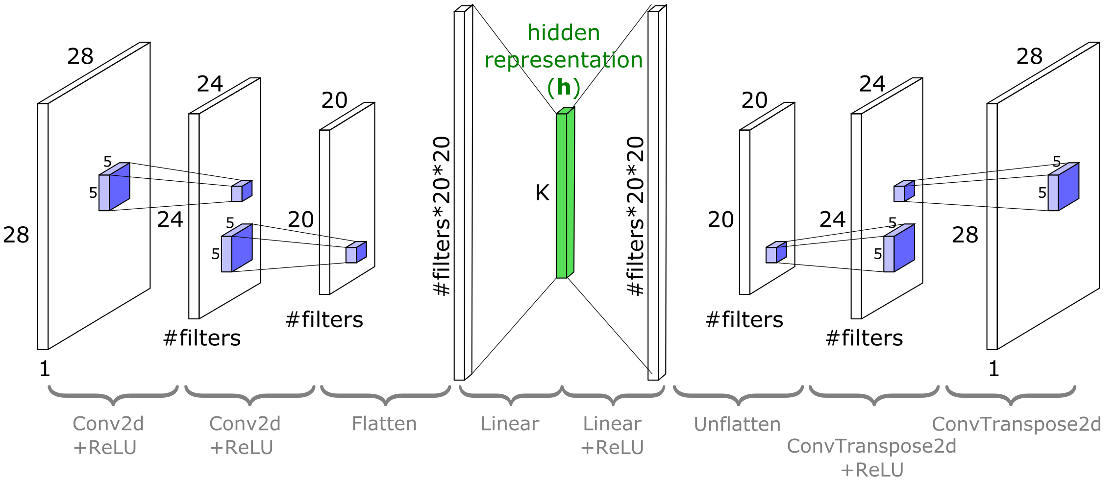
    return x + self.bias

それでは、非線形かつ畳み込みのオートエンコーダを定義しましょう。アーキテクチャの概要は以下の通りです：

エンコーダは再び画像から $\mathbf{h}\in\mathbb{R}^K$ へマッピングします。BiasLayerの後に2つの畳み込み層（nn.Conv2D）が続き、その後フラット化して $K$ 次元に線形射影します。畳み込み層の出力にはReLU非線形性が適用されます。
デコーダはこの処理を逆に行い、長さ $K$ のベクトルから画像を出力します。大まかにはエンコーダの「鏡像」構造で、最初のデコーダ層は線形、その後に2つの逆畳み込み層（ConvTranspose2d）があります。ConvTranspose2d層の入力にはReLU非線形性が適用されます。このエンコーダとデコーダの「鏡像」構造は便利でほぼ普遍的な慣習です。デコーダはエンコーダを近似的に逆に学習できますが、厳密な逆関数になるわけではありませんし、保証もありません。

以下はMNIST用のアーキテクチャの概略図です。nn.Conv2dの後に画像の幅と高さが減少し、nn.ConvTranspose2dの後に増加することに注意してください。CIFAR10では同じアーキテクチャですが具体的なサイズは異なります。

torch.nn.ConvTranspose2dモジュールは、Conv2dの入力に関する勾配として見ることができます。これは分数ストライド畳み込みや逆畳み込みとも呼ばれます（ただし実際の逆畳み込み演算ではありません）。以下のコードはサイズの変化を示しています。

dummy_image = torch.rand(data_shape).unsqueeze(0)
in_channels = data_shape[0]
out_channels = 7

dummy_conv = nn.Conv2d(in_channels=in_channels,
                       out_channels=out_channels,
                       kernel_size=5)

dummy_deconv = nn.ConvTranspose2d(in_channels=out_channels,
                                  out_channels=in_channels,
                                  kernel_size=5)

print(f'Size of image is {dummy_image.shape}')
print(f'Size of Conv2D(image) {dummy_conv(dummy_image).shape}')
print(f'Size of ConvTranspose2D(Conv2D(image)) {dummy_deconv(dummy_conv(dummy_image)).shape}')

コーディング演習 3.2: `ConvAutoEncoder`モジュールのコードを完成させよう

ConvAutoEncoderクラスを完成させてください。ヘルパー関数cout(torch.Tensor, nn.Conv2D)は、形状(channels, height, width)のテンソルに対してnn.Conv2D層の出力形状を計算します。

ここで使うKの値はコーディング演習3.1で定義したものを使います。最終的に線形オートエンコーダとこの畳み込みオートエンコーダの結果を比較するためです。Kを変えたい場合は3.1で変更し、両方のオートエンコーダを再学習してください。

畳み込みオートエンコーダと線形オートエンコーダのどちらが平均二乗誤差（MSE）をより低くできると思いますか？

class ConvAutoEncoder(nn.Module):
  """
  A Convolutional AutoEncoder
  """

  def __init__(self, x_dim, h_dim, n_filters=32, filter_size=5):
    """
    Initialize parameters of ConvAutoEncoder

    Args:
      x_dim: tuple
        Input dimensions (channels, height, widths)
      h_dim: int
        Hidden dimension, bottleneck dimension, K
      n_filters: int
        Number of filters (number of output channels)
      filter_size: int
        Kernel size

    Returns:
      Nothing
    """
    super().__init__()
    channels, height, widths = x_dim

    # Encoder input bias layer
    self.enc_bias = BiasLayer(x_dim)

    # First encoder conv2d layer
    self.enc_conv_1 = nn.Conv2d(channels, n_filters, filter_size)

    # Output shape of the first encoder conv2d layer given x_dim input
    conv_1_shape = cout(x_dim, self.enc_conv_1)

    # Second encoder conv2d layer
    self.enc_conv_2 = nn.Conv2d(n_filters, n_filters, filter_size)

    # Output shape of the second encoder conv2d layer given conv_1_shape input
    conv_2_shape = cout(conv_1_shape, self.enc_conv_2)

    # The bottleneck is a dense layer, therefore we need a flattenning layer
    self.enc_flatten = nn.Flatten()

    # Conv output shape is (depth, height, width), so the flatten size is:
    flat_after_conv = conv_2_shape[0] * conv_2_shape[1] * conv_2_shape[2]

    # Encoder Linear layer
    self.enc_lin = nn.Linear(flat_after_conv, h_dim)

    ####################################################################
    # Fill in all missing code below (...),
    # then remove or comment the line below to test your class
    # Remember that decoder is "undo"-ing what the encoder has done!
    raise NotImplementedError("Please complete the `ConvAutoEncoder` class!")
    ####################################################################
    # Decoder Linear layer
    self.dec_lin = ...

    # Unflatten data to (depth, height, width) shape
    self.dec_unflatten = nn.Unflatten(dim=-1, unflattened_size=conv_2_shape)

    # First "deconvolution" layer
    self.dec_deconv_1 = nn.ConvTranspose2d(n_filters, n_filters, filter_size)

    # Second "deconvolution" layer
    self.dec_deconv_2 = ...

    # Decoder output bias layer
    self.dec_bias = BiasLayer(x_dim)

  def encode(self, x):
    """
    Encoder

    Args:
      x: torch.tensor
        Input features

    Returns:
      h: torch.tensor
        Encoded output
    """
    s = self.enc_bias(x)
    s = F.relu(self.enc_conv_1(s))
    s = F.relu(self.enc_conv_2(s))
    s = self.enc_flatten(s)
    h = self.enc_lin(s)
    return h

  def decode(self, h):
    """
    Decoder

    Args:
      h: torch.tensor
        Encoded output

    Returns:
      x_prime: torch.tensor
        Decoded output
    """
    s = F.relu(self.dec_lin(h))
    s = self.dec_unflatten(s)
    s = F.relu(self.dec_deconv_1(s))
    s = self.dec_deconv_2(s)
    x_prime = self.dec_bias(s)
    return x_prime

  def forward(self, x):
    """
    Forward pass

    Args:
      x: torch.tensor
        Input features

    Returns:
      Decoded output
    """
    return self.decode(self.encode(x))



set_seed(seed=SEED)
## Uncomment to test your solution
# trained_conv_AE = ConvAutoEncoder(data_shape, K)
# assert trained_conv_AE.encode(train_set[0][0].unsqueeze(0)).numel() == K, "Encoder output size should be K!"
# conv_losses = train_autoencoder(trained_conv_AE, train_set, device=DEVICE, seed=SEED)
# plot_conv_ae(lin_losses, conv_losses)

解答を見る$

ConvAutoEncoderが線形のものよりも低いMSE損失を達成していることがわかるはずです。もしそうでなければ、再度訓練するか（または途中から数エポック追加で訓練を行う）必要があるかもしれません。CIFAR10ではうまくいく保証は少ないですが、MNISTでは確実に機能するはずです。

では、線形オートエンコーダと非線形オートエンコーダの再構成画像を視覚的に比較してみましょう。両者とも $\mathbf{h}$ の次元数は同じであることに注意してください。

# @markdown Visualize the linear and nonlinear AE outputs
if lin_ae.enc_lin.out_features != trained_conv_AE.enc_lin.out_features:
   raise ValueError('ERROR: your linear and convolutional autoencoders have different values of K')

n_plot = 7
plt.figure(figsize=(10, 4.5))
for i in range(n_plot):
  idx = torch.randint(len(train_set), size=())
  image, _ = train_set[idx]
  with torch.no_grad():
    # Get reconstructed image from linear autoencoder
    lin_recon = lin_ae(image.unsqueeze(0))[0]

    # Get reconstruction from deep (nonlinear) autoencoder
    nonlin_recon = trained_conv_AE(image.unsqueeze(0))[0]

  plt.subplot(3, n_plot, i+1)
  plot_torch_image(image)
  if i == 0:
    plt.ylabel('Original\nImage')

  plt.subplot(3, n_plot, i + 1 + n_plot)
  plot_torch_image(lin_recon)
  if i == 0:
    plt.ylabel(f'Lin AE\n(K={K})')

  plt.subplot(3, n_plot, i + 1 + 2*n_plot)
  plot_torch_image(nonlin_recon)
  if i == 0:
    plt.ylabel(f'NonLin AE\n(K={K})')
plt.show()

# @title Submit your feedback
content_review(f"{feedback_prefix}_NonLinear_AutoEncoder_Exercise")

セクション4: 変分オートエンコーダ（VAE）

所要時間の目安: 約25分

動画の後にセルを実行して、MNIST用のVAEを訓練してください。動画を見ながら行うことを推奨します。

# @title Video 4: Variational Autoencoders
from ipywidgets import widgets
from IPython.display import YouTubeVideo
from IPython.display import IFrame
from IPython.display import display


class PlayVideo(IFrame):
  def __init__(self, id, source, page=1, width=400, height=300, **kwargs):
    self.id = id
    if source == 'Bilibili':
      src = f'https://player.bilibili.com/player.html?bvid={id}&page={page}'
    elif source == 'Osf':
      src = f'https://mfr.ca-1.osf.io/render?url=https://osf.io/download/{id}/?direct%26mode=render'
    super(PlayVideo, self).__init__(src, width, height, **kwargs)


def display_videos(video_ids, W=400, H=300, fs=1):
  tab_contents = []
  for i, video_id in enumerate(video_ids):
    out = widgets.Output()
    with out:
      if video_ids[i][0] == 'Youtube':
        video = YouTubeVideo(id=video_ids[i][1], width=W,
                             height=H, fs=fs, rel=0)
        print(f'Video available at https://youtube.com/watch?v={video.id}')
      else:
        video = PlayVideo(id=video_ids[i][1], source=video_ids[i][0], width=W,
                          height=H, fs=fs, autoplay=False)
        if video_ids[i][0] == 'Bilibili':
          print(f'Video available at https://www.bilibili.com/video/{video.id}')
        elif video_ids[i][0] == 'Osf':
          print(f'Video available at https://osf.io/{video.id}')
      display(video)
    tab_contents.append(out)
  return tab_contents


video_ids = [('Youtube', 'srWb_Gp6OGA'), ('Bilibili', 'BV17v411E7ye')]
tab_contents = display_videos(video_ids, W=854, H=480)
tabs = widgets.Tab()
tabs.children = tab_contents
for i in range(len(tab_contents)):
  tabs.set_title(i, video_ids[i][0])
display(tabs)

# @title Submit your feedback
content_review(f"{feedback_prefix}_Variational_AutoEncoder_Video")

# @markdown Train a VAE for MNIST while watching the video. (Note: this VAE has a 2D latent space. If you are feeling ambitious, edit the code and modify the latent space dimensionality and see what happens.)
K_VAE = 2


class ConvVAE(nn.Module):
  """
  Convolutional Variational Autoencoder
  """
  def __init__(self, K, num_filters=32, filter_size=5):
    """
    Initialize parameters of ConvVAE

    Args:
      K: int
        Bottleneck dimensionality
      num_filters: int
        Number of filters [default: 32]
      filter_size: int
        Filter size [default: 5]

    Returns:
      Nothing
    """

    super(ConvVAE, self).__init__()

    # With padding=0, the number of pixels cut off from
    # each image dimension
    # is filter_size // 2. Double it to get the amount
    # of pixels lost in
    # width and height per Conv2D layer, or added back
    # in per
    # ConvTranspose2D layer.
    filter_reduction = 2 * (filter_size // 2)

    # After passing input through two Conv2d layers,
    # the shape will be
    # 'shape_after_conv'. This is also the shape that
    # will go into the first
    # deconvolution layer in the decoder
    self.shape_after_conv = (num_filters,
                              data_shape[1]-2*filter_reduction,
                              data_shape[2]-2*filter_reduction)
    flat_size_after_conv = self.shape_after_conv[0] \
        * self.shape_after_conv[1] \
        * self.shape_after_conv[2]

    # Define the recognition model (encoder or q) part
    self.q_bias = BiasLayer(data_shape)
    self.q_conv_1 = nn.Conv2d(data_shape[0], num_filters, 5)
    self.q_conv_2 = nn.Conv2d(num_filters, num_filters, 5)
    self.q_flatten = nn.Flatten()
    self.q_fc_phi = nn.Linear(flat_size_after_conv, K+1)

    # Define the generative model (decoder or p) part
    self.p_fc_upsample = nn.Linear(K, flat_size_after_conv)
    self.p_unflatten = nn.Unflatten(-1, self.shape_after_conv)
    self.p_deconv_1 = nn.ConvTranspose2d(num_filters, num_filters, 5)
    self.p_deconv_2 = nn.ConvTranspose2d(num_filters, data_shape[0], 5)
    self.p_bias = BiasLayer(data_shape)

    # Define a special extra parameter to learn
    # scalar sig_x for all pixels
    self.log_sig_x = nn.Parameter(torch.zeros(()))

  def infer(self, x):
    """
    Map (batch of) x to (batch of) phi which
    can then be passed to
    rsample to get z

    Args:
      x: torch.tensor
        Input features

    Returns:
      phi: np.ndarray
        Relative entropy
    """
    s = self.q_bias(x)
    s = F.relu(self.q_conv_1(s))
    s = F.relu(self.q_conv_2(s))
    flat_s = s.view(s.size()[0], -1)
    phi = self.q_fc_phi(flat_s)
    return phi

  def generate(self, zs):
    """
    Map [b,n,k] sized samples of z to
    [b,n,p] sized images

    Args:
      zs: np.ndarray
        Samples

    Returns:
      mu_zs: np.ndarray
        Mean of samples
    """
    # Note that for the purposes of passing
    # through the generator, we need
    # to reshape zs to be size [b*n,k]
    b, n, k = zs.size()
    s = zs.view(b*n, -1)
    s = F.relu(self.p_fc_upsample(s)).view((b*n,) + self.shape_after_conv)
    s = F.relu(self.p_deconv_1(s))
    s = self.p_deconv_2(s)
    s = self.p_bias(s)
    mu_xs = s.view(b, n, -1)
    return mu_xs

  def decode(self, zs):
    """
    Decoder

    Args:
      zs: np.ndarray
        Samples

    Returns:
      Generated images
    """
    # Included for compatability with conv-AE code
    return self.generate(zs.unsqueeze(0))

  def forward(self, x):
    """
    Forward pass

    Args:
      x: torch.tensor
        Input image

    Returns:
      Generated images
    """
    # VAE.forward() is not used for training,
    # but we'll treat it like a
    # classic autoencoder by taking a single
    # sample of z ~ q
    phi = self.infer(x)
    zs = rsample(phi, 1)
    return self.generate(zs).view(x.size())

  def elbo(self, x, n=1):
    """
    Run input end to end through the VAE
    and compute the ELBO using n
    samples of z

    Args:
      x: torch.tensor
        Input image
      n: int
        Number of samples of z

    Returns:
      Difference between true and estimated KL divergence
    """
    phi = self.infer(x)
    zs = rsample(phi, n)
    mu_xs = self.generate(zs)
    return log_p_x(x, mu_xs, self.log_sig_x.exp()) - kl_q_p(zs, phi)


def expected_z(phi):
  """
  Expected sample entropy

  Args:
    phi: list
      Relative entropy

  Returns:
    Expected sample entropy
  """
  return phi[:, :-1]


def rsample(phi, n_samples):
  """
  Sample z ~ q(z;phi)
  Output z is size [b,n_samples,K] given
  phi with shape [b,K+1]. The first K
  entries of each row of phi are the mean of q,
  and phi[:,-1] is the log
  standard deviation

  Args:
    phi: list
      Relative entropy
    n_samples: int
      Number of samples

  Returns:
    Output z is size [b,n_samples,K] given
  phi with shape [b,K+1]. The first K
  entries of each row of phi are the mean of q,
  and phi[:,-1] is the log
  standard deviation
  """
  b, kplus1 = phi.size()
  k = kplus1-1
  mu, sig = phi[:, :-1], phi[:,-1].exp()
  eps = torch.randn(b, n_samples, k, device=phi.device)
  return eps*sig.view(b,1,1) + mu.view(b,1,k)


def train_vae(vae, dataset, epochs=10, n_samples=1000):
  """
  Train VAE

  Args:
    vae: nn.module
      Model
    dataset: function
      Dataset
    epochs: int
      Epochs
    n_samples: int
      Number of samples

  Returns:
    elbo_vals: list
      List of values obtained from ELBO
  """
  opt = torch.optim.Adam(vae.parameters(), lr=1e-3, weight_decay=0)
  elbo_vals = []
  vae.to(DEVICE)
  vae.train()
  loader = DataLoader(dataset, batch_size=250, shuffle=True, pin_memory=True)
  for epoch in trange(epochs, desc='Epochs'):
    for im, _ in tqdm(loader, total=len(dataset) // 250, desc='Batches', leave=False):
      im = im.to(DEVICE)
      opt.zero_grad()
      loss = -vae.elbo(im)
      loss.backward()
      opt.step()

      elbo_vals.append(-loss.item())
  vae.to('cpu')
  vae.eval()
  return elbo_vals


trained_conv_VarAE = ConvVAE(K=K_VAE)
elbo_vals = train_vae(trained_conv_VarAE, train_set, n_samples=10000)

print(f'Learned sigma_x is {torch.exp(trained_conv_VarAE.log_sig_x)}')

# Uncomment below if you'd like to see the the training
# curve of the evaluated ELBO loss function
# ELBO is the loss function used to train VAEs
# (see lecture!)
plt.figure()
plt.plot(elbo_vals)
plt.xlabel('Batch #')
plt.ylabel('ELBO')
plt.show()

ELBOはVAEの訓練に用いられる損失関数です。ELBOを最大化する（ELBOが高いほど良い）ことを目指します。PyTorchのコードでは損失を負のELBOに設定して最小化する形で実装しています。

セクション4.1: VAEの構成要素

認識モデルと密度ネットワーク

変分オートエンコーダ（VAE）は古典的なオートエンコーダ（AE）に似ていますが、確率分布を明示的に扱う点が異なります。VAEの用語では、__エンコーダ__は__認識モデル__に置き換えられ、__デコーダ__は__密度ネットワーク__に置き換えられます。

古典的なオートエンコーダでは、エンコーダは画像から単一の隠れベクトルへマッピングします。

\mathbf{x} \overset{\text{AE}}{\longrightarrow} \mathbf{h} \, ,

一方、VAEでは認識モデルが入力から隠れベクトルの__分布全体__へマッピングします。

\mathbf{x} \overset{\text{VAE}}{\longrightarrow} q_{\mathbf{w_e}}(\mathbf{z}) \, ,

ここからサンプリングを行います。 $\mathbf{w_e}$ は認識モデルの重みで、この分布生成ネットワークのパラメータを指します。 $q_{\mathbf{w_e}}(\mathbf{z})$ がどのような分布かについては後ほど詳しく説明します。
VAEが機能する理由の一つは、損失関数が単一の $\mathbf{z}$ だけでなく、 $\mathbf{z} \sim q_{\mathbf{w_e}}(\mathbf{z})$ からのサンプルの平均的な再構成の良さを要求する点にあります。

古典的なオートエンコーダでは、デコーダは隠れベクトルから入力の再構成へマッピングします。

\mathbf{h} \overset{\text{AE}}{\longrightarrow} \mathbf{x'} \, .

密度ネットワークでは、再構成は分布として表現されます。

\mathbf{z} \overset{\text{VAE}}{\longrightarrow} p_{\mathbf{w_d}}(\mathbf{x}|\mathbf{z})

ここで、 $p_{\mathbf{w_d}}(\mathbf{x}|\mathbf{z})$ は $\mathbf{z}$ を密度ネットワークに通し、得られた $f(\mathbf{z};\mathbf{w_d})$ を $\mathbf{x}$ の（ガウス）分布の平均として扱うことで定義されます。同様に、再構成分布は密度ネットワークの重みでパラメータ化されます。

セクション4.2: デコーダから新規画像を生成する

オートエンコーダのデコーダ部分だけを取り出すと、入力としてサイズ $K$ のベクトルを受け取り、訓練データに似た画像を出力するニューラルネットワークになります。先ほどの表記では、入力 $\mathbf{x}$ が低次元の隠れ表現 $\mathbf{h}$ にマッピングされ、さらにそれが入力の再構成 $\mathbf{x'}$ にデコードされました。

\mathbf{x} \overset{\text{encode}}{\longrightarrow} \mathbf{h} \overset{\text{decode}}{\longrightarrow} \mathbf{x'}\, .

慣習的な理由と、次に進む内容を前節と区別するために、新たに $\mathbf{z} \in \mathbb{R}^K$ という変数を導入します。 $\mathbf{h}$ は特定の $\mathbf{x}$ に対してエンコーダが生成しますが、 $\mathbf{z}$ は任意の事前分布から自由にサンプリングされます。

\mathbf{z} \sim p(\mathbf{z})\\ \mathbf{z} \overset{\text{decode}}{\longrightarrow} \mathbf{x}\, .

（なお、 $\mathbf{x}$ がもはや「再構成」として扱われない場合、 $\mathbf{x'}$ のプライム記号を省略するのが一般的です。）

コーディング演習4.2: 画像生成

以下のコードを完成させて、上で訓練したVAEから画像を生成してください。

def generate_images(autoencoder, K, n_images=1):
  """
  Generate n_images 'new' images from the decoder part of the given
  autoencoder.

  Args:
    autoencoder: nn.module
      Autoencoder model
    K: int
      Bottleneck dimension
    n_images: int
      Number of images

  Returns:
    x: torch.tensor
      (n_images, channels, height, width) tensor of images
  """
  # Concatenate tuples to get (n_images, channels, height, width)
  output_shape = (n_images,) + data_shape
  with torch.no_grad():
    ####################################################################
    # Fill in all missing code below (...),
    # then remove or comment the line below to test your function
    raise NotImplementedError("Please complete the `generate_images` function!")
    ####################################################################
    # Sample z from a unit gaussian, pass through autoencoder.decode()
    z = ...
    x = ...

    return x.reshape(output_shape)



set_seed(seed=SEED)
## Uncomment to test your solution
# images = generate_images(trained_conv_AE, K, n_images=9)
# plot_images(images, plt_title='Images Generated from the Conv-AE')
# images = generate_images(trained_conv_VarAE, K_VAE, n_images=9)
# plot_images(images, plt_title='Images Generated from a Conv-Variational-AE')

解答を見る$

# @title Submit your feedback
content_review(f"{feedback_prefix}_Generating_images_Exercise")

考えてみよう！4.2: オートエンコーダと変分オートエンコーダの比較

オートエンコーダで生成した画像と変分オートエンコーダで生成した画像を比較してください。コードを何度か実行して様々な例を見てみましょう。

どちらの画像群が訓練セット（手書き数字）により似ていますか？その違いは何によって生じているのでしょうか？

解答を見る$

# @title Submit your feedback
content_review(f"{feedback_prefix}_AutoEncoders_vs_Variational_AutoEncoders_Discussion")

セクション5: 最先端のVAEとまとめ

# @title Video 5: State-Of-The-Art VAEs
from ipywidgets import widgets
from IPython.display import YouTubeVideo
from IPython.display import IFrame
from IPython.display import display


class PlayVideo(IFrame):
  def __init__(self, id, source, page=1, width=400, height=300, **kwargs):
    self.id = id
    if source == 'Bilibili':
      src = f'https://player.bilibili.com/player.html?bvid={id}&page={page}'
    elif source == 'Osf':
      src = f'https://mfr.ca-1.osf.io/render?url=https://osf.io/download/{id}/?direct%26mode=render'
    super(PlayVideo, self).__init__(src, width, height, **kwargs)


def display_videos(video_ids, W=400, H=300, fs=1):
  tab_contents = []
  for i, video_id in enumerate(video_ids):
    out = widgets.Output()
    with out:
      if video_ids[i][0] == 'Youtube':
        video = YouTubeVideo(id=video_ids[i][1], width=W,
                             height=H, fs=fs, rel=0)
        print(f'Video available at https://youtube.com/watch?v={video.id}')
      else:
        video = PlayVideo(id=video_ids[i][1], source=video_ids[i][0], width=W,
                          height=H, fs=fs, autoplay=False)
        if video_ids[i][0] == 'Bilibili':
          print(f'Video available at https://www.bilibili.com/video/{video.id}')
        elif video_ids[i][0] == 'Osf':
          print(f'Video available at https://osf.io/{video.id}')
      display(video)
    tab_contents.append(out)
  return tab_contents


video_ids = [('Youtube', 'PXBl3KwRfh4'), ('Bilibili', 'BV1hg411M7KY')]
tab_contents = display_videos(video_ids, W=854, H=480)
tabs = widgets.Tab()
tabs.children = tab_contents
for i in range(len(tab_contents)):
  tabs.set_title(i, video_ids[i][0])
display(tabs)

# @title Submit your feedback
content_review(f"{feedback_prefix}_SOTA_VAEs_and_WrapUp_Video")

まとめ

このチュートリアルを通じて、以下を学びました。

生成モデルとは何か、なぜそれに関心があるのか。
pPCAの例を通じて、潜在変数モデルが生成モデルとどのように関連するか。
基本的なオートエンコーダとは何か、そしてそれが他の潜在変数モデルとどのように関係するか。
変分オートエンコーダの基礎と、それが生成モデルとしてどのように機能するか。
VAEの幅広い応用の入門。

チュートリアル 1: 変分オートエンコーダ（VAE）

チュートリアルの目標

セットアップ

セクション 1: 生成モデル

セクション 1.1: BigGANからの画像生成

インタラクティブデモ 1.1: BigGANジェネレーター

考えてみよう！1.1: 生成された画像

セクション 1.2: BigGANによる画像の補間

インタラクティブデモ 1.2: BigGAN補間

考えてみよう！1.2: 同じカテゴリのサンプル間の補間

セクション 2: 潜在変数モデル

（ボーナス）コーディング演習 2: pPCA

セクション 3: オートエンコーダー

データセットを選択

セクション 3.1: オートエンコーダーの概念的導入

コーディング演習 3.1: 線形オートエンコーダのアーキテクチャ

PCAとの比較

考えてみよう 3.1: PCAと線形オートエンコーダの比較

セクション 3.2: 非線形畳み込みオートエンコーダの構築

コーディング演習 3.2: ConvAutoEncoderモジュールのコードを完成させよう

セクション4: 変分オートエンコーダ（VAE）

セクション4.1: VAEの構成要素

セクション4.2: デコーダから新規画像を生成する

コーディング演習4.2: 画像生成

考えてみよう！4.2: オートエンコーダと変分オートエンコーダの比較

セクション5: 最先端のVAEとまとめ

まとめ

コーディング演習 3.2: `ConvAutoEncoder`モジュールのコードを完成させよう