チュートリアル 1: モダンな畳み込みネットワークの使い方を学ぼう

第2週、第3日目: モダンな畳み込みネットワーク

Neuromatch Academyによる

コンテンツ作成者: Laura Pede, Richard Vogg, Marissa Weis, Timo Lüddecke, Alexander Ecker

コンテンツレビュアー: Arush Tagade, Polina Turishcheva, Yu-Fang Yang, Bettina Hein, Melvin Selim Atay, Kelson Shilling-Scrivo

コンテンツ編集者: Gagana B, Roberto Guidotti, Spiros Chavlis

制作編集者: Anoop Kulkarni, Roberto Guidotti, Cary Murray, Gagana B, Spiros Chavlis

チュートリアルノートブックはBen Heilによる初期バージョンを基にしています

チュートリアルの目的

このチュートリアルでは、畳み込みネットワーク（ConvNet）についてさらに学びます。具体的には、以下のことを行います。

1. モダンなCNNと転移学習について学ぶ。
2. アーキテクチャがどのように世界に関する私たちの知識を取り入れているか理解する。
3. モダンなCNNの基本的な構成要素の動作原理を理解する。
4. 転移学習の概念を理解し、それを適用する機会を認識できるようになる。
5. （ボーナス）速度と精度のトレードオフを理解する。

# @title Tutorial slides
from IPython.display import IFrame
link_id = "tzfsn"
print(f"If you want to download the slides: https://osf.io/download/{link_id}/")
IFrame(src=f"https://mfr.ca-1.osf.io/render?url=https://osf.io/{link_id}/?direct%26mode=render%26action=download%26mode=render", width=854, height=480)

セットアップ

# @title Install dependencies

# @title Install and import feedback gadget


from vibecheck import DatatopsContentReviewContainer
def content_review(notebook_section: str):
    return DatatopsContentReviewContainer(
        "",  # No text prompt
        notebook_section,
        {
            "url": "https://pmyvdlilci.execute-api.us-east-1.amazonaws.com/klab",
            "name": "neuromatch_dl",
            "user_key": "f379rz8y",
        },
    ).render()


feedback_prefix = "W2D3_T1"

# Import libraries
import os
import time
import tqdm
import torch
import IPython
import torchvision

import numpy as np
import matplotlib.pyplot as plt

import torch.nn as nn
import torch.nn.functional as F

from torchvision import transforms
from torchvision.models import AlexNet
from torchvision.utils import make_grid
from torchvision.datasets import ImageFolder

from PIL import Image
from io import BytesIO

# @title Figure settings
import logging
logging.getLogger('matplotlib.font_manager').disabled = True

import ipywidgets as widgets  # Interactive display
%config InlineBackend.figure_format = 'retina'
plt.style.use("https://raw.githubusercontent.com/NeuromatchAcademy/content-creation/main/nma.mplstyle")

# @title Set random seed

# @markdown Executing `set_seed(seed=seed)` you are setting the seed

# For DL its critical to set the random seed so that students can have a
# baseline to compare their results to expected results.
# Read more here: https://pytorch.org/docs/stable/notes/randomness.html

# Call `set_seed` function in the exercises to ensure reproducibility.
import random
import torch

def set_seed(seed=None, seed_torch=True):
  """
  Function that controls randomness. NumPy and random modules must be imported.

  Args:
    seed : Integer
      A non-negative integer that defines the random state. Default is `None`.
    seed_torch : Boolean
      If `True` sets the random seed for pytorch tensors, so pytorch module
      must be imported. Default is `True`.

  Returns:
    Nothing.
  """
  if seed is None:
    seed = np.random.choice(2 ** 32)
  random.seed(seed)
  np.random.seed(seed)
  if seed_torch:
    torch.manual_seed(seed)
    torch.cuda.manual_seed_all(seed)
    torch.cuda.manual_seed(seed)
    torch.backends.cudnn.benchmark = False
    torch.backends.cudnn.deterministic = True

  print(f'Random seed {seed} has been set.')


# In case that `DataLoader` is used
def seed_worker(worker_id):
  """
  DataLoader will reseed workers following randomness in
  multi-process data loading algorithm.

  Args:
    worker_id: integer
      ID of subprocess to seed. 0 means that
      the data will be loaded in the main process
      Refer: https://pytorch.org/docs/stable/data.html#data-loading-randomness for more details

  Returns:
    Nothing
  """
  worker_seed = torch.initial_seed() % 2**32
  np.random.seed(worker_seed)
  random.seed(worker_seed)

# @title Set device (GPU or CPU). Execute `set_device()`
# especially if torch modules used.

# Inform the user if the notebook uses GPU or CPU.

def set_device():
  """
  Set the device. CUDA if available, CPU otherwise

  Args:
    None

  Returns:
    Nothing
  """
  device = "cuda" if torch.cuda.is_available() else "cpu"
  if device != "cuda":
    print("WARNING: For this notebook to perform best, "
        "if possible, in the menu under `Runtime` -> "
        "`Change runtime type.`  select `GPU` ")
  else:
    print("GPU is enabled in this notebook.")

  return device

SEED = 2021
set_seed(seed=SEED)
DEVICE = set_device()

セクション1: モダンなCNNと転移学習

所要時間の目安: 約25分

# @title Video 1: Modern CNNs and Transfer Learning
from ipywidgets import widgets
from IPython.display import YouTubeVideo
from IPython.display import IFrame
from IPython.display import display


class PlayVideo(IFrame):
  def __init__(self, id, source, page=1, width=400, height=300, **kwargs):
    self.id = id
    if source == 'Bilibili':
      src = f'https://player.bilibili.com/player.html?bvid={id}&page={page}'
    elif source == 'Osf':
      src = f'https://mfr.ca-1.osf.io/render?url=https://osf.io/download/{id}/?direct%26mode=render'
    super(PlayVideo, self).__init__(src, width, height, **kwargs)


def display_videos(video_ids, W=400, H=300, fs=1):
  tab_contents = []
  for i, video_id in enumerate(video_ids):
    out = widgets.Output()
    with out:
      if video_ids[i][0] == 'Youtube':
        video = YouTubeVideo(id=video_ids[i][1], width=W,
                             height=H, fs=fs, rel=0)
        print(f'Video available at https://youtube.com/watch?v={video.id}')
      else:
        video = PlayVideo(id=video_ids[i][1], source=video_ids[i][0], width=W,
                          height=H, fs=fs, autoplay=False)
        if video_ids[i][0] == 'Bilibili':
          print(f'Video available at https://www.bilibili.com/video/{video.id}')
        elif video_ids[i][0] == 'Osf':
          print(f'Video available at https://osf.io/{video.id}')
      display(video)
    tab_contents.append(out)
  return tab_contents


video_ids = [('Youtube', 'mfOd2EKzscM'), ('Bilibili', 'BV1Wf4y157wE')]
tab_contents = display_videos(video_ids, W=854, H=480)
tabs = widgets.Tab()
tabs.children = tab_contents
for i in range(len(tab_contents)):
  tabs.set_title(i, video_ids[i][0])
display(tabs)

# @title Submit your feedback
content_review(f"{feedback_prefix}_Modern_CNNs_and_Transfer_Learning_Video")

画像は高次元です。つまり、image_length * image_width * image_channels は大きな数になり、その大きな数に通常サイズの全結合層を掛けると、学習すべきパラメータ数が膨大になります。昨日は、画像や他のドメインの高次元性を回避する方法の一つとして畳み込みニューラルネットワーク（CNN）について学びました。

以下のウィジェット（インタラクティブデモ1）は、特定の高さと幅の画像に対して動作する単一の畳み込み層または全結合層に必要なパラメータ数を計算します。

畳み込み層$l$のパラメータ数は以下のように計算されることを思い出してください。

ここで、$H$はフィルターの高さの形状、$W$はフィルターの幅の形状、$K_l$は$l$層目のフィルター数を表します。加算されている$1$は各フィルターのバイアス項のためです。

一方、全結合層のパラメータ数は以下の通りです。

ここで、$N_l$は$l$層目のノード数を表します。

スライダーを調整して、異なるモデルやデータの特性がモデルが学習すべきパラメータ数にどのように影響するかの直感を得ましょう。

注：これらのクラスはネットワークの最初の層におけるパラメータのスケーリングを示すために設計されており、実際に有用にするにはより多くの層や活性化関数などが必要です。

class FullyConnectedNet(nn.Module):
  """
  Fully connected network with the following structure:
  nn.Linear(self.input_size, 256)
  """

  def __init__(self):
    """
    Initialize parameters of FullyConnectedNet

    Args:
      None

    Returns:
      Nothing
    """
    super(FullyConnectedNet, self).__init__()

    image_width = 128
    image_channels = 3
    self.input_size = image_channels * image_width ** 2

    self.fc1 = nn.Linear(self.input_size, 256)

  def forward(self, x):
    """
    Forward pass of FullyConnectedNet

    Args:
      x: torch.tensor
        Input data

    Returns:
      x: torch.tensor
        Output from FullyConnectedNet
    """
    x = x.view(-1, self.input_size)
    return self.fc1(x)

class ConvNet(nn.Module):
  """
  Convolutional Neural Network
  """

  def __init__(self):
    """
    Initialize parameters of ConvNet

    Args:
      None

    Returns:
      Nothing
    """
    super(ConvNet, self).__init__()

    self.conv1 = nn.Conv2d(in_channels=3,
                            out_channels=256,
                            kernel_size=(3, 3),
                            padding=1)

  def forward(self, x):
    """
    Forward pass of ConvNet

    Args:
      x: torch.tensor
        Input data

    Returns:
      x: torch.tensor
        Output after passing x through Conv2d layer
    """
    return self.conv1(x)

コーディング演習1: FCNNとConvNetのパラメータ数を計算しよう

与えられたネットワークのパラメータ数を計算する関数を書きましょう。上で定義した全結合ネットワークと畳み込みネットワークにその関数を適用し、パラメータ数を比較してください。

ヒント: torch.numel

def get_parameter_count(network):
  """
  Calculate the number of parameters used by the fully connected/convolutional network.
  Hint: Casting the result of network.parameters() to a list may make it
        easier to work with

  Args:
    network: nn.module
      Network to calculate the parameters of fully connected/convolutional network

  Returns:
    param_count: int
      The number of parameters in the network
  """

  ####################################################################
  # Fill in all missing code below (...),
  # then remove or comment the line below to test your function
  raise NotImplementedError("Convolution math")
  ####################################################################
  # Get the network's parameters
  parameters = ...

  param_count = 0
  # Loop over all layers
  for layer in parameters:
    param_count += ...

  return param_count



# Initialize networks
fccnet = FullyConnectedNet()
convnet = ConvNet()
## Apply the above defined function to both networks by uncommenting the following lines
# print(f"FCCN parameter count: {get_parameter_count(fccnet)}")
# print(f"ConvNet parameter count: {get_parameter_count(convnet)}")

FCCNのパラメータ数: 12583168
ConvNetのパラメータ数: 7168

解答を見る$

# @title Submit your feedback
content_review(f"{feedback_prefix}_Calculate_number_of_params_Exercise")

インタラクティブデモ1: 結果を確認しよう

以下のウィジェットは、上記のモデルと同じアーキテクチャを持つFCNNとCNNのパラメータ数を計算します。私たちのモデルは入力画像が128x128で、256個のフィルター（またはFCNNの場合は256個のノード）を使っていました。上で計算した値が正しいか確認してください。

入力画像サイズを大きくしても、畳み込みネットワークのパラメータ数が非常に少ないことに注目してください。

# @title Parameter Calculator
# @markdown Run this cell to enable the widget!

def calculate_parameters(filter_count, image_width,
                         fcnn_nodes):
  """
  Implement how parameters
  scale as a function of image size
  between convnets and FCNN

  Args:
    filter_count: int
      Number of filters
    image_width: int
      Width of image
    fcnn_nodes: int
      Number of fCNN nodes

  Returns:
    None
  """

  filter_width = 3
  image_channels = 3

  # Assuming a square, RGB image
  image_area = image_width ** 2
  image_volume = image_area * image_channels

  # If we're using padding=same, the output of a
  # convnet will be the same shape
  # as the original image, but with more features
  fcnn_parameters = image_volume * fcnn_nodes
  cnn_parameters = image_channels * filter_count * filter_width ** 2

  # Add bias
  fcnn_parameters += fcnn_nodes
  cnn_parameters += filter_count

  print(f"CNN parameters: {cnn_parameters}")
  print(f"Fully Connected parameters: {fcnn_parameters}")

  return None


_ = widgets.interact(calculate_parameters,
                     filter_count=(16, 512, 16),
                     image_width=(16, 512, 16),
                     fcnn_nodes=(16, 512, 16))

# @title Submit your feedback
content_review(f"{feedback_prefix}_Check_your_results_Interactive_Demo")

セクション2: 畳み込みネットワークの歴史

所要時間の目安: 約15分

畳み込みニューラルネットワークは長い歴史があります。最初のCNNモデルは1980年に発表され、それ以前の数十年にわたる神経科学のアイデアに基づいていました。では、なぜ2012年に発表されたCNNモデルのAlexNetがディープラーニング革命の始まりと一般的に考えられているのでしょうか？

以下のビデオを見て、ハードウェアとインターネットがディープラーニングの進展に果たした役割を理解しましょう。

# @title Video 2: History of convnets
from ipywidgets import widgets
from IPython.display import YouTubeVideo
from IPython.display import IFrame
from IPython.display import display


class PlayVideo(IFrame):
  def __init__(self, id, source, page=1, width=400, height=300, **kwargs):
    self.id = id
    if source == 'Bilibili':
      src = f'https://player.bilibili.com/player.html?bvid={id}&page={page}'
    elif source == 'Osf':
      src = f'https://mfr.ca-1.osf.io/render?url=https://osf.io/download/{id}/?direct%26mode=render'
    super(PlayVideo, self).__init__(src, width, height, **kwargs)


def display_videos(video_ids, W=400, H=300, fs=1):
  tab_contents = []
  for i, video_id in enumerate(video_ids):
    out = widgets.Output()
    with out:
      if video_ids[i][0] == 'Youtube':
        video = YouTubeVideo(id=video_ids[i][1], width=W,
                             height=H, fs=fs, rel=0)
        print(f'Video available at https://youtube.com/watch?v={video.id}')
      else:
        video = PlayVideo(id=video_ids[i][1], source=video_ids[i][0], width=W,
                          height=H, fs=fs, autoplay=False)
        if video_ids[i][0] == 'Bilibili':
          print(f'Video available at https://www.bilibili.com/video/{video.id}')
        elif video_ids[i][0] == 'Osf':
          print(f'Video available at https://osf.io/{video.id}')
      display(video)
    tab_contents.append(out)
  return tab_contents


video_ids = [('Youtube', 'xtoLjKSPrUQ'), ('Bilibili', 'BV1364y167Qy')]
tab_contents = display_videos(video_ids, W=854, H=480)
tabs = widgets.Tab()
tabs.children = tab_contents
for i in range(len(tab_contents)):
  tabs.set_title(i, video_ids[i][0])
display(tabs)

# @title Submit your feedback
content_review(f"{feedback_prefix}_History_of_convnets_Video")

考えよう！2: CNNを改良する際の課題

今日学ぶように、ディープラーニングとCNNの歴史はネットワークのスケールアップ、つまりより大きく深くすることの歴史でした。

これまでの学びを踏まえて、研究者たちがCNNをスケールアップし、さまざまな視覚認識タスクに適用する際に直面した課題は何だと思いますか？これらの課題がどのように解決されたかについて、すでに何かアイデアはありますか？

グループで約10分間話し合ってみましょう。

（ヒント：ラベル付きデータ、計算資源、メモリはいずれも有限です）

解答を見る$

# @title Submit your feedback
content_review(f"{feedback_prefix}_Challenges_of_improving_CNNs_Discussion")

セクション3: 大規模で深い畳み込みネットワーク

所要時間の目安: 18分

# @title Video 3: AlexNet & VGG
from ipywidgets import widgets
from IPython.display import YouTubeVideo
from IPython.display import IFrame
from IPython.display import display


class PlayVideo(IFrame):
  def __init__(self, id, source, page=1, width=400, height=300, **kwargs):
    self.id = id
    if source == 'Bilibili':
      src = f'https://player.bilibili.com/player.html?bvid={id}&page={page}'
    elif source == 'Osf':
      src = f'https://mfr.ca-1.osf.io/render?url=https://osf.io/download/{id}/?direct%26mode=render'
    super(PlayVideo, self).__init__(src, width, height, **kwargs)


def display_videos(video_ids, W=400, H=300, fs=1):
  tab_contents = []
  for i, video_id in enumerate(video_ids):
    out = widgets.Output()
    with out:
      if video_ids[i][0] == 'Youtube':
        video = YouTubeVideo(id=video_ids[i][1], width=W,
                             height=H, fs=fs, rel=0)
        print(f'Video available at https://youtube.com/watch?v={video.id}')
      else:
        video = PlayVideo(id=video_ids[i][1], source=video_ids[i][0], width=W,
                          height=H, fs=fs, autoplay=False)
        if video_ids[i][0] == 'Bilibili':
          print(f'Video available at https://www.bilibili.com/video/{video.id}')
        elif video_ids[i][0] == 'Osf':
          print(f'Video available at https://osf.io/{video.id}')
      display(video)
    tab_contents.append(out)
  return tab_contents


video_ids = [('Youtube', 'ZB87qC7yPiE'), ('Bilibili', 'BV12U4y1n7q5')]
tab_contents = display_videos(video_ids, W=854, H=480)
tabs = widgets.Tab()
tabs.children = tab_contents
for i in range(len(tab_contents)):
  tabs.set_title(i, video_ids[i][0])
display(tabs)

# @title Submit your feedback
content_review(f"{feedback_prefix}_AlexNet_and_VGG_Video")

セクション3.1: AlexNetの紹介

AlexNetは現在のディープラーニング時代の始まりを象徴すると言えます。
それは、深いネットワーク、GPUによる並列処理、タスク固有の事前知識を組み込んだ構成要素など、今日の成功したDLの特徴を多く取り入れています。
このセクションではAlexNetを操作し、その視点から世界を見る機会があります。

# @title Import Alexnet
# @markdown This cell gives you the `alexnet` model as well as the `input_image` and `input_batch` variables used below
import requests, urllib

# Original link: https://s3.amazonaws.com/pytorch/models/alexnet-owt-4df8aa71.pth
state_dict = torch.hub.load_state_dict_from_url("https://osf.io/9dzeu/download")

alexnet = AlexNet()
alexnet.load_state_dict(state_dict=state_dict)

url, filename = ("https://raw.githubusercontent.com/NeuromatchAcademy/course-content-dl/main/tutorials/W2D3_ModernConvnets/static/dog.jpg", "dog.jpg")
try: urllib.URLopener().retrieve(url, filename)
except: urllib.request.urlretrieve(url, filename)

input_image = Image.open(filename)
preprocess = transforms.Compose([
                                 transforms.Resize(256),
                                 transforms.CenterCrop(224),
                                 transforms.ToTensor(),
                                 transforms.Normalize(mean=[0.485, 0.456, 0.406],
                                                      std=[0.229, 0.224, 0.225]),
                                 ])
input_tensor = preprocess(input_image)
input_batch = input_tensor.unsqueeze(0)  # Create a mini-batch as expected by the model

# Move the input and model to GPU for speed if available
if torch.cuda.is_available():
  input_batch = input_batch.cuda()
  alexnet.cuda()

セクション 3.2: AlexNet は何を学習しているのか？

このコードは AlexNet が学習した最上層のフィルターを可視化します。
これらのフィルターは何を思い起こさせますか？

with torch.no_grad():
  params = list(alexnet.parameters())
  fig, axs = plt.subplots(8, 8, figsize=(8, 8))
  filters = []
  for filter_index in range(params[0].shape[0]):
    row_index = filter_index // 8
    col_index = filter_index % 8

    filter = params[0][filter_index,:,:,:]
    filter_image = filter.permute(1, 2, 0).cpu()
    scale = np.abs(filter_image).max()
    scaled_image = filter_image / (2 * scale) + 0.5
    filters.append(scaled_image.cpu())
    axs[row_index, col_index].imshow(scaled_image.cpu())
    axs[row_index, col_index].axis('off')
  plt.show()

考えてみよう！3.2.1: フィルターの類似性

これらのフィルターは何を思い起こさせますか？

解答を見る$

# @title Submit your feedback
content_review(f"{feedback_prefix}_Filter_Similarity_Discussion")

インタラクティブデモ 3.2: AlexNet は何を見ているのか？

CNN を可視化する一つの方法は、特定の画像に対する個々のフィルターの出力を見ることです。以下のウィジェットでは、AlexNet で使われている様々なフィルターの出力を調べることができます。

# @markdown Run this cell to enable the widget

def alexnet_intermediate_output(net, image):
    """
    Function to extract AlexNet's intermediate output

    Args:
      net: nn.module
        AlexNet instance
      image: torch.tensor
        Input features

    Returns:
      ReLU output on processing features
    """
    return F.relu(net.features[0](image))


def browse_images(input_batch, input_image):
  """
  Helper function to browse images

  Args:
    input_batch: torch.tensor
      Input batch
    input_image: torch.tensor
      Input features

  Returns:
    Nothing
  """
  intermediate_output = alexnet_intermediate_output(alexnet, input_batch)
  n = intermediate_output.shape[1]

  def view_image(i):
    """
    Function to view incoming image frame

    Args:
      i: int
        Iteration

    Returns:
      Nothing
    """
    with torch.no_grad():
      channel = intermediate_output[0, i, :].squeeze()
      fig, ax = plt.subplots(1, 3, figsize=(12, 6))
      ax[0].imshow(input_image)
      ax[1].imshow(filters[i])
      ax[1].set_xlim([-22, 33])
      ax[2].imshow(channel.cpu())
      ax[0].set_title('Input image')
      ax[1].set_title(f"Filter {i}")
      ax[2].set_title(f"Filter {i} on input image")
      [axi.set_axis_off() for axi in ax.ravel()]

  widgets.interact(view_image, i=(0, n-1))


browse_images(input_batch, input_image)

# @title Submit your feedback
content_review(f"{feedback_prefix}_What_does_AlexNet_see_Interactive_Demo")

考えてみよう！3.2.2 フィルターの役割

これらのフィルターは何をしているように見えますか？異なるフィルターは異なる役割を果たしているため、いくつかの良い答えがあります。

解答を見る$

# @title Submit your feedback
content_review(f"{feedback_prefix}_Filter_Purpose_Discussion")

さらなる読み物

「ニューラルネットワークのフィルターは何を探しているのか？」という問いに興味がある方や、幾何学的なアートが好きな方には、様々な CNN ニューロンの出力を最大化する画像を作成したこちらの記事がおすすめです。また、モデルの学習過程で画像空間がどのように変化するかを示した良い記事もこちらにあります。

セクション 4: AlexNet 後の畳み込みネットワーク

所要時間の目安: 約25分

# @title Video 4: Residual Networks (ResNets)
from ipywidgets import widgets
from IPython.display import YouTubeVideo
from IPython.display import IFrame
from IPython.display import display


class PlayVideo(IFrame):
  def __init__(self, id, source, page=1, width=400, height=300, **kwargs):
    self.id = id
    if source == 'Bilibili':
      src = f'https://player.bilibili.com/player.html?bvid={id}&page={page}'
    elif source == 'Osf':
      src = f'https://mfr.ca-1.osf.io/render?url=https://osf.io/download/{id}/?direct%26mode=render'
    super(PlayVideo, self).__init__(src, width, height, **kwargs)


def display_videos(video_ids, W=400, H=300, fs=1):
  tab_contents = []
  for i, video_id in enumerate(video_ids):
    out = widgets.Output()
    with out:
      if video_ids[i][0] == 'Youtube':
        video = YouTubeVideo(id=video_ids[i][1], width=W,
                             height=H, fs=fs, rel=0)
        print(f'Video available at https://youtube.com/watch?v={video.id}')
      else:
        video = PlayVideo(id=video_ids[i][1], source=video_ids[i][0], width=W,
                          height=H, fs=fs, autoplay=False)
        if video_ids[i][0] == 'Bilibili':
          print(f'Video available at https://www.bilibili.com/video/{video.id}')
        elif video_ids[i][0] == 'Osf':
          print(f'Video available at https://osf.io/{video.id}')
      display(video)
    tab_contents.append(out)
  return tab_contents


video_ids = [('Youtube', 'EJSZnJyy4PI'), ('Bilibili', 'BV1bf4y1j7od')]
tab_contents = display_videos(video_ids, W=854, H=480)
tabs = widgets.Tab()
tabs.children = tab_contents
for i in range(len(tab_contents)):
  tabs.set_title(i, video_ids[i][0])
display(tabs)

# @title Submit your feedback
content_review(f"{feedback_prefix}_Residual_Networks_ResNets_Video")

このセクションでは、最先端の CNN モデルであるResNetを扱います。ResNet には特に興味深い特徴が二つあります。まず、スキップ接続を使って勾配消失問題を回避していること。次に、ResNet の各ブロック（複数の層の集合）は残差関数を学習するものとして扱えることです。

数学的に言うと、ニューラルネットワークは入力（例えば犬の画像）から出力（例えば「犬」というラベル）への写像を行う一連の操作と考えられます。数学用語では、入力から出力への写像を関数と呼びます。ニューラルネットワークはその関数を表現する柔軟な方法です。

もしネットワークが学習した関数から、画像をクラスラベルに写像する真の関数を引き算すると、残差誤差または「残差関数」が残ります。ResNet は元の関数を学習し、その後に残差関数、さらに残差の残差を学習し続けることを目指しており、これを残差ブロックを使って前の層の出力に加算しています。

このセクションでは、事前学習済みの ResNet に複数の画像を通して何が起こるかを見ていきます。

# @title Download imagenette
import requests, tarfile, os

fname = 'imagenette2-320'
url = 'https://osf.io/mnve4/download'

if not os.path.exists(fname):
  print("Data is being downloaded...")
  r = requests.get(url, stream=True)
  with open(fname+'tgz', 'wb') as fd:
    fd.write(r.content)

  with tarfile.open(fname+'tgz', "r") as ft:
    ft.extractall()

  os.remove(fname+'tgz')
  print("The download has been completed.")
else:
  print("Data has already been downloaded.")

# @title Set Up Textual ImageNet labels
dict_map={0: 'tench, Tinca tinca',
 1: 'goldfish, Carassius auratus',
 2: 'great white shark, white shark, man-eater, man-eating shark, Carcharodon carcharias',
 3: 'tiger shark, Galeocerdo cuvieri',
 4: 'hammerhead, hammerhead shark',
 5: 'electric ray, crampfish, numbfish, torpedo',
 6: 'stingray',
 7: 'cock',
 8: 'hen',
 9: 'ostrich, Struthio camelus',
 10: 'brambling, Fringilla montifringilla',
 11: 'goldfinch, Carduelis carduelis',
 12: 'house finch, linnet, Carpodacus mexicanus',
 13: 'junco, snowbird',
 14: 'indigo bunting, indigo finch, indigo bird, Passerina cyanea',
 15: 'robin, American robin, Turdus migratorius',
 16: 'bulbul',
 17: 'jay',
 18: 'magpie',
 19: 'chickadee',
 20: 'water ouzel, dipper',
 21: 'kite',
 22: 'bald eagle, American eagle, Haliaeetus leucocephalus',
 23: 'vulture',
 24: 'great grey owl, great gray owl, Strix nebulosa',
 25: 'European fire salamander, Salamandra salamandra',
 26: 'common newt, Triturus vulgaris',
 27: 'eft',
 28: 'spotted salamander, Ambystoma maculatum',
 29: 'axolotl, mud puppy, Ambystoma mexicanum',
 30: 'bullfrog, Rana catesbeiana',
 31: 'tree frog, tree-frog',
 32: 'tailed frog, bell toad, ribbed toad, tailed toad, Ascaphus trui',
 33: 'loggerhead, loggerhead turtle, Caretta caretta',
 34: 'leatherback turtle, leatherback, leathery turtle, Dermochelys coriacea',
 35: 'mud turtle',
 36: 'terrapin',
 37: 'box turtle, box tortoise',
 38: 'banded gecko',
 39: 'common iguana, iguana, Iguana iguana',
 40: 'American chameleon, anole, Anolis carolinensis',
 41: 'whiptail, whiptail lizard',
 42: 'agama',
 43: 'frilled lizard, Chlamydosaurus kingi',
 44: 'alligator lizard',
 45: 'Gila monster, Heloderma suspectum',
 46: 'green lizard, Lacerta viridis',
 47: 'African chameleon, Chamaeleo chamaeleon',
 48: 'Komodo dragon, Komodo lizard, dragon lizard, giant lizard, Varanus komodoensis',
 49: 'African crocodile, Nile crocodile, Crocodylus niloticus',
 50: 'American alligator, Alligator mississipiensis',
 51: 'triceratops',
 52: 'thunder snake, worm snake, Carphophis amoenus',
 53: 'ringneck snake, ring-necked snake, ring snake',
 54: 'hognose snake, puff adder, sand viper',
 55: 'green snake, grass snake',
 56: 'king snake, kingsnake',
 57: 'garter snake, grass snake',
 58: 'water snake',
 59: 'vine snake',
 60: 'night snake, Hypsiglena torquata',
 61: 'boa constrictor, Constrictor constrictor',
 62: 'rock python, rock snake, Python sebae',
 63: 'Indian cobra, Naja naja',
 64: 'green mamba',
 65: 'sea snake',
 66: 'horned viper, cerastes, sand viper, horned asp, Cerastes cornutus',
 67: 'diamondback, diamondback rattlesnake, Crotalus adamanteus',
 68: 'sidewinder, horned rattlesnake, Crotalus cerastes',
 69: 'trilobite',
 70: 'harvestman, daddy longlegs, Phalangium opilio',
 71: 'scorpion',
 72: 'black and gold garden spider, Argiope aurantia',
 73: 'barn spider, Araneus cavaticus',
 74: 'garden spider, Aranea diademata',
 75: 'black widow, Latrodectus mactans',
 76: 'tarantula',
 77: 'wolf spider, hunting spider',
 78: 'tick',
 79: 'centipede',
 80: 'black grouse',
 81: 'ptarmigan',
 82: 'ruffed grouse, partridge, Bonasa umbellus',
 83: 'prairie chicken, prairie grouse, prairie fowl',
 84: 'peacock',
 85: 'quail',
 86: 'partridge',
 87: 'African grey, African gray, Psittacus erithacus',
 88: 'macaw',
 89: 'sulphur-crested cockatoo, Kakatoe galerita, Cacatua galerita',
 90: 'lorikeet',
 91: 'coucal',
 92: 'bee eater',
 93: 'hornbill',
 94: 'hummingbird',
 95: 'jacamar',
 96: 'toucan',
 97: 'drake',
 98: 'red-breasted merganser, Mergus serrator',
 99: 'goose',
 100: 'black swan, Cygnus atratus',
 101: 'tusker',
 102: 'echidna, spiny anteater, anteater',
 103: 'platypus, duckbill, duckbilled platypus, duck-billed platypus, Ornithorhynchus anatinus',
 104: 'wallaby, brush kangaroo',
 105: 'koala, koala bear, kangaroo bear, native bear, Phascolarctos cinereus',
 106: 'wombat',
 107: 'jellyfish',
 108: 'sea anemone, anemone',
 109: 'brain coral',
 110: 'flatworm, platyhelminth',
 111: 'nematode, nematode worm, roundworm',
 112: 'conch',
 113: 'snail',
 114: 'slug',
 115: 'sea slug, nudibranch',
 116: 'chiton, coat-of-mail shell, sea cradle, polyplacophore',
 117: 'chambered nautilus, pearly nautilus, nautilus',
 118: 'Dungeness crab, Cancer magister',
 119: 'rock crab, Cancer irroratus',
 120: 'fiddler crab',
 121: 'king crab, Alaska crab, Alaskan king crab, Alaska king crab, Paralithodes camtschatica',
 122: 'American lobster, Northern lobster, Maine lobster, Homarus americanus',
 123: 'spiny lobster, langouste, rock lobster, crawfish, crayfish, sea crawfish',
 124: 'crayfish, crawfish, crawdad, crawdaddy',
 125: 'hermit crab',
 126: 'isopod',
 127: 'white stork, Ciconia ciconia',
 128: 'black stork, Ciconia nigra',
 129: 'spoonbill',
 130: 'flamingo',
 131: 'little blue heron, Egretta caerulea',
 132: 'American egret, great white heron, Egretta albus',
 133: 'bittern',
 134: 'crane',
 135: 'limpkin, Aramus pictus',
 136: 'European gallinule, Porphyrio porphyrio',
 137: 'American coot, marsh hen, mud hen, water hen, Fulica americana',
 138: 'bustard',
 139: 'ruddy turnstone, Arenaria interpres',
 140: 'red-backed sandpiper, dunlin, Erolia alpina',
 141: 'redshank, Tringa totanus',
 142: 'dowitcher',
 143: 'oystercatcher, oyster catcher',
 144: 'pelican',
 145: 'king penguin, Aptenodytes patagonica',
 146: 'albatross, mollymawk',
 147: 'grey whale, gray whale, devilfish, Eschrichtius gibbosus, Eschrichtius robustus',
 148: 'killer whale, killer, orca, grampus, sea wolf, Orcinus orca',
 149: 'dugong, Dugong dugon',
 150: 'sea lion',
 151: 'Chihuahua',
 152: 'Japanese spaniel',
 153: 'Maltese dog, Maltese terrier, Maltese',
 154: 'Pekinese, Pekingese, Peke',
 155: 'Shih-Tzu',
 156: 'Blenheim spaniel',
 157: 'papillon',
 158: 'toy terrier',
 159: 'Rhodesian ridgeback',
 160: 'Afghan hound, Afghan',
 161: 'basset, basset hound',
 162: 'beagle',
 163: 'bloodhound, sleuthhound',
 164: 'bluetick',
 165: 'black-and-tan coonhound',
 166: 'Walker hound, Walker foxhound',
 167: 'English foxhound',
 168: 'redbone',
 169: 'borzoi, Russian wolfhound',
 170: 'Irish wolfhound',
 171: 'Italian greyhound',
 172: 'whippet',
 173: 'Ibizan hound, Ibizan Podenco',
 174: 'Norwegian elkhound, elkhound',
 175: 'otterhound, otter hound',
 176: 'Saluki, gazelle hound',
 177: 'Scottish deerhound, deerhound',
 178: 'Weimaraner',
 179: 'Staffordshire bullterrier, Staffordshire bull terrier',
 180: 'American Staffordshire terrier, Staffordshire terrier, American pit bull terrier, pit bull terrier',
 181: 'Bedlington terrier',
 182: 'Border terrier',
 183: 'Kerry blue terrier',
 184: 'Irish terrier',
 185: 'Norfolk terrier',
 186: 'Norwich terrier',
 187: 'Yorkshire terrier',
 188: 'wire-haired fox terrier',
 189: 'Lakeland terrier',
 190: 'Sealyham terrier, Sealyham',
 191: 'Airedale, Airedale terrier',
 192: 'cairn, cairn terrier',
 193: 'Australian terrier',
 194: 'Dandie Dinmont, Dandie Dinmont terrier',
 195: 'Boston bull, Boston terrier',
 196: 'miniature schnauzer',
 197: 'giant schnauzer',
 198: 'standard schnauzer',
 199: 'Scotch terrier, Scottish terrier, Scottie',
 200: 'Tibetan terrier, chrysanthemum dog',
 201: 'silky terrier, Sydney silky',
 202: 'soft-coated wheaten terrier',
 203: 'West Highland white terrier',
 204: 'Lhasa, Lhasa apso',
 205: 'flat-coated retriever',
 206: 'curly-coated retriever',
 207: 'golden retriever',
 208: 'Labrador retriever',
 209: 'Chesapeake Bay retriever',
 210: 'German short-haired pointer',
 211: 'vizsla, Hungarian pointer',
 212: 'English setter',
 213: 'Irish setter, red setter',
 214: 'Gordon setter',
 215: 'Brittany spaniel',
 216: 'clumber, clumber spaniel',
 217: 'English springer, English springer spaniel',
 218: 'Welsh springer spaniel',
 219: 'cocker spaniel, English cocker spaniel, cocker',
 220: 'Sussex spaniel',
 221: 'Irish water spaniel',
 222: 'kuvasz',
 223: 'schipperke',
 224: 'groenendael',
 225: 'malinois',
 226: 'briard',
 227: 'kelpie',
 228: 'komondor',
 229: 'Old English sheepdog, bobtail',
 230: 'Shetland sheepdog, Shetland sheep dog, Shetland',
 231: 'collie',
 232: 'Border collie',
 233: 'Bouvier des Flandres, Bouviers des Flandres',
 234: 'Rottweiler',
 235: 'German shepherd, German shepherd dog, German police dog, alsatian',
 236: 'Doberman, Doberman pinscher',
 237: 'miniature pinscher',
 238: 'Greater Swiss Mountain dog',
 239: 'Bernese mountain dog',
 240: 'Appenzeller',
 241: 'EntleBucher',
 242: 'boxer',
 243: 'bull mastiff',
 244: 'Tibetan mastiff',
 245: 'French bulldog',
 246: 'Great Dane',
 247: 'Saint Bernard, St Bernard',
 248: 'Eskimo dog, husky',
 249: 'malamute, malemute, Alaskan malamute',
 250: 'Siberian husky',
 251: 'dalmatian, coach dog, carriage dog',
 252: 'affenpinscher, monkey pinscher, monkey dog',
 253: 'basenji',
 254: 'pug, pug-dog',
 255: 'Leonberg',
 256: 'Newfoundland, Newfoundland dog',
 257: 'Great Pyrenees',
 258: 'Samoyed, Samoyede',
 259: 'Pomeranian',
 260: 'chow, chow chow',
 261: 'keeshond',
 262: 'Brabancon griffon',
 263: 'Pembroke, Pembroke Welsh corgi',
 264: 'Cardigan, Cardigan Welsh corgi',
 265: 'toy poodle',
 266: 'miniature poodle',
 267: 'standard poodle',
 268: 'Mexican hairless',
 269: 'timber wolf, grey wolf, gray wolf, Canis lupus',
 270: 'white wolf, Arctic wolf, Canis lupus tundrarum',
 271: 'red wolf, maned wolf, Canis rufus, Canis niger',
 272: 'coyote, prairie wolf, brush wolf, Canis latrans',
 273: 'dingo, warrigal, warragal, Canis dingo',
 274: 'dhole, Cuon alpinus',
 275: 'African hunting dog, hyena dog, Cape hunting dog, Lycaon pictus',
 276: 'hyena, hyaena',
 277: 'red fox, Vulpes vulpes',
 278: 'kit fox, Vulpes macrotis',
 279: 'Arctic fox, white fox, Alopex lagopus',
 280: 'grey fox, gray fox, Urocyon cinereoargenteus',
 281: 'tabby, tabby cat',
 282: 'tiger cat',
 283: 'Persian cat',
 284: 'Siamese cat, Siamese',
 285: 'Egyptian cat',
 286: 'cougar, puma, catamount, mountain lion, painter, panther, Felis concolor',
 287: 'lynx, catamount',
 288: 'leopard, Panthera pardus',
 289: 'snow leopard, ounce, Panthera uncia',
 290: 'jaguar, panther, Panthera onca, Felis onca',
 291: 'lion, king of beasts, Panthera leo',
 292: 'tiger, Panthera tigris',
 293: 'cheetah, chetah, Acinonyx jubatus',
 294: 'brown bear, bruin, Ursus arctos',
 295: 'American black bear, black bear, Ursus americanus, Euarctos americanus',
 296: 'ice bear, polar bear, Ursus Maritimus, Thalarctos maritimus',
 297: 'sloth bear, Melursus ursinus, Ursus ursinus',
 298: 'mongoose',
 299: 'meerkat, mierkat',
 300: 'tiger beetle',
 301: 'ladybug, ladybeetle, lady beetle, ladybird, ladybird beetle',
 302: 'ground beetle, carabid beetle',
 303: 'long-horned beetle, longicorn, longicorn beetle',
 304: 'leaf beetle, chrysomelid',
 305: 'dung beetle',
 306: 'rhinoceros beetle',
 307: 'weevil',
 308: 'fly',
 309: 'bee',
 310: 'ant, emmet, pismire',
 311: 'grasshopper, hopper',
 312: 'cricket',
 313: 'walking stick, walkingstick, stick insect',
 314: 'cockroach, roach',
 315: 'mantis, mantid',
 316: 'cicada, cicala',
 317: 'leafhopper',
 318: 'lacewing, lacewing fly',
 319: "dragonfly, darning needle, devil's darning needle, sewing needle, snake feeder, snake doctor, mosquito hawk, skeeter hawk",
 320: 'damselfly',
 321: 'admiral',
 322: 'ringlet, ringlet butterfly',
 323: 'monarch, monarch butterfly, milkweed butterfly, Danaus plexippus',
 324: 'cabbage butterfly',
 325: 'sulphur butterfly, sulfur butterfly',
 326: 'lycaenid, lycaenid butterfly',
 327: 'starfish, sea star',
 328: 'sea urchin',
 329: 'sea cucumber, holothurian',
 330: 'wood rabbit, cottontail, cottontail rabbit',
 331: 'hare',
 332: 'Angora, Angora rabbit',
 333: 'hamster',
 334: 'porcupine, hedgehog',
 335: 'fox squirrel, eastern fox squirrel, Sciurus niger',
 336: 'marmot',
 337: 'beaver',
 338: 'guinea pig, Cavia cobaya',
 339: 'sorrel',
 340: 'zebra',
 341: 'hog, pig, grunter, squealer, Sus scrofa',
 342: 'wild boar, boar, Sus scrofa',
 343: 'warthog',
 344: 'hippopotamus, hippo, river horse, Hippopotamus amphibius',
 345: 'ox',
 346: 'water buffalo, water ox, Asiatic buffalo, Bubalus bubalis',
 347: 'bison',
 348: 'ram, tup',
 349: 'bighorn, bighorn sheep, cimarron, Rocky Mountain bighorn, Rocky Mountain sheep, Ovis canadensis',
 350: 'ibex, Capra ibex',
 351: 'hartebeest',
 352: 'impala, Aepyceros melampus',
 353: 'gazelle',
 354: 'Arabian camel, dromedary, Camelus dromedarius',
 355: 'llama',
 356: 'weasel',
 357: 'mink',
 358: 'polecat, fitch, foulmart, foumart, Mustela putorius',
 359: 'black-footed ferret, ferret, Mustela nigripes',
 360: 'otter',
 361: 'skunk, polecat, wood pussy',
 362: 'badger',
 363: 'armadillo',
 364: 'three-toed sloth, ai, Bradypus tridactylus',
 365: 'orangutan, orang, orangutang, Pongo pygmaeus',
 366: 'gorilla, Gorilla gorilla',
 367: 'chimpanzee, chimp, Pan troglodytes',
 368: 'gibbon, Hylobates lar',
 369: 'siamang, Hylobates syndactylus, Symphalangus syndactylus',
 370: 'guenon, guenon monkey',
 371: 'patas, hussar monkey, Erythrocebus patas',
 372: 'baboon',
 373: 'macaque',
 374: 'langur',
 375: 'colobus, colobus monkey',
 376: 'proboscis monkey, Nasalis larvatus',
 377: 'marmoset',
 378: 'capuchin, ringtail, Cebus capucinus',
 379: 'howler monkey, howler',
 380: 'titi, titi monkey',
 381: 'spider monkey, Ateles geoffroyi',
 382: 'squirrel monkey, Saimiri sciureus',
 383: 'Madagascar cat, ring-tailed lemur, Lemur catta',
 384: 'indri, indris, Indri indri, Indri brevicaudatus',
 385: 'Indian elephant, Elephas maximus',
 386: 'African elephant, Loxodonta africana',
 387: 'lesser panda, red panda, panda, bear cat, cat bear, Ailurus fulgens',
 388: 'giant panda, panda, panda bear, coon bear, Ailuropoda melanoleuca',
 389: 'barracouta, snoek',
 390: 'eel',
 391: 'coho, cohoe, coho salmon, blue jack, silver salmon, Oncorhynchus kisutch',
 392: 'rock beauty, Holocanthus tricolor',
 393: 'anemone fish',
 394: 'sturgeon',
 395: 'gar, garfish, garpike, billfish, Lepisosteus osseus',
 396: 'lionfish',
 397: 'puffer, pufferfish, blowfish, globefish',
 398: 'abacus',
 399: 'abaya',
 400: "academic gown, academic robe, judge's robe",
 401: 'accordion, piano accordion, squeeze box',
 402: 'acoustic guitar',
 403: 'aircraft carrier, carrier, flattop, attack aircraft carrier',
 404: 'airliner',
 405: 'airship, dirigible',
 406: 'altar',
 407: 'ambulance',
 408: 'amphibian, amphibious vehicle',
 409: 'analog clock',
 410: 'apiary, bee house',
 411: 'apron',
 412: 'ashcan, trash can, garbage can, wastebin, ash bin, ash-bin, ashbin, dustbin, trash barrel, trash bin',
 413: 'assault rifle, assault gun',
 414: 'backpack, back pack, knapsack, packsack, rucksack, haversack',
 415: 'bakery, bakeshop, bakehouse',
 416: 'balance beam, beam',
 417: 'balloon',
 418: 'ballpoint, ballpoint pen, ballpen, Biro',
 419: 'Band Aid',
 420: 'banjo',
 421: 'bannister, banister, balustrade, balusters, handrail',
 422: 'barbell',
 423: 'barber chair',
 424: 'barbershop',
 425: 'barn',
 426: 'barometer',
 427: 'barrel, cask',
 428: 'barrow, garden cart, lawn cart, wheelbarrow',
 429: 'baseball',
 430: 'basketball',
 431: 'bassinet',
 432: 'bassoon',
 433: 'bathing cap, swimming cap',
 434: 'bath towel',
 435: 'bathtub, bathing tub, bath, tub',
 436: 'beach wagon, station wagon, wagon, estate car, beach waggon, station waggon, waggon',
 437: 'beacon, lighthouse, beacon light, pharos',
 438: 'beaker',
 439: 'bearskin, busby, shako',
 440: 'beer bottle',
 441: 'beer glass',
 442: 'bell cote, bell cot',
 443: 'bib',
 444: 'bicycle-built-for-two, tandem bicycle, tandem',
 445: 'bikini, two-piece',
 446: 'binder, ring-binder',
 447: 'binoculars, field glasses, opera glasses',
 448: 'birdhouse',
 449: 'boathouse',
 450: 'bobsled, bobsleigh, bob',
 451: 'bolo tie, bolo, bola tie, bola',
 452: 'bonnet, poke bonnet',
 453: 'bookcase',
 454: 'bookshop, bookstore, bookstall',
 455: 'bottlecap',
 456: 'bow',
 457: 'bow tie, bow-tie, bowtie',
 458: 'brass, memorial tablet, plaque',
 459: 'brassiere, bra, bandeau',
 460: 'breakwater, groin, groyne, mole, bulwark, seawall, jetty',
 461: 'breastplate, aegis, egis',
 462: 'broom',
 463: 'bucket, pail',
 464: 'buckle',
 465: 'bulletproof vest',
 466: 'bullet train, bullet',
 467: 'butcher shop, meat market',
 468: 'cab, hack, taxi, taxicab',
 469: 'caldron, cauldron',
 470: 'candle, taper, wax light',
 471: 'cannon',
 472: 'canoe',
 473: 'can opener, tin opener',
 474: 'cardigan',
 475: 'car mirror',
 476: 'carousel, carrousel, merry-go-round, roundabout, whirligig',
 477: "carpenter's kit, tool kit",
 478: 'carton',
 479: 'car wheel',
 480: 'cash machine, cash dispenser, automated teller machine, automatic teller machine, automated teller, automatic teller, ATM',
 481: 'cassette',
 482: 'cassette player',
 483: 'castle',
 484: 'catamaran',
 485: 'CD player',
 486: 'cello, violoncello',
 487: 'cellular telephone, cellular phone, cellphone, cell, mobile phone',
 488: 'chain',
 489: 'chainlink fence',
 490: 'chain mail, ring mail, mail, chain armor, chain armour, ring armor, ring armour',
 491: 'chain saw, chainsaw',
 492: 'chest',
 493: 'chiffonier, commode',
 494: 'chime, bell, gong',
 495: 'china cabinet, china closet',
 496: 'Christmas stocking',
 497: 'church, church building',
 498: 'cinema, movie theater, movie theatre, movie house, picture palace',
 499: 'cleaver, meat cleaver, chopper',
 500: 'cliff dwelling',
 501: 'cloak',
 502: 'clog, geta, patten, sabot',
 503: 'cocktail shaker',
 504: 'coffee mug',
 505: 'coffeepot',
 506: 'coil, spiral, volute, whorl, helix',
 507: 'combination lock',
 508: 'computer keyboard, keypad',
 509: 'confectionery, confectionary, candy store',
 510: 'container ship, containership, container vessel',
 511: 'convertible',
 512: 'corkscrew, bottle screw',
 513: 'cornet, horn, trumpet, trump',
 514: 'cowboy boot',
 515: 'cowboy hat, ten-gallon hat',
 516: 'cradle',
 517: 'crane',
 518: 'crash helmet',
 519: 'crate',
 520: 'crib, cot',
 521: 'Crock Pot',
 522: 'croquet ball',
 523: 'crutch',
 524: 'cuirass',
 525: 'dam, dike, dyke',
 526: 'desk',
 527: 'desktop computer',
 528: 'dial telephone, dial phone',
 529: 'diaper, nappy, napkin',
 530: 'digital clock',
 531: 'digital watch',
 532: 'dining table, board',
 533: 'dishrag, dishcloth',
 534: 'dishwasher, dish washer, dishwashing machine',
 535: 'disk brake, disc brake',
 536: 'dock, dockage, docking facility',
 537: 'dogsled, dog sled, dog sleigh',
 538: 'dome',
 539: 'doormat, welcome mat',
 540: 'drilling platform, offshore rig',
 541: 'drum, membranophone, tympan',
 542: 'drumstick',
 543: 'dumbbell',
 544: 'Dutch oven',
 545: 'electric fan, blower',
 546: 'electric guitar',
 547: 'electric locomotive',
 548: 'entertainment center',
 549: 'envelope',
 550: 'espresso maker',
 551: 'face powder',
 552: 'feather boa, boa',
 553: 'file, file cabinet, filing cabinet',
 554: 'fireboat',
 555: 'fire engine, fire truck',
 556: 'fire screen, fireguard',
 557: 'flagpole, flagstaff',
 558: 'flute, transverse flute',
 559: 'folding chair',
 560: 'football helmet',
 561: 'forklift',
 562: 'fountain',
 563: 'fountain pen',
 564: 'four-poster',
 565: 'freight car',
 566: 'French horn, horn',
 567: 'frying pan, frypan, skillet',
 568: 'fur coat',
 569: 'garbage truck, dustcart',
 570: 'gasmask, respirator, gas helmet',
 571: 'gas pump, gasoline pump, petrol pump, island dispenser',
 572: 'goblet',
 573: 'go-kart',
 574: 'golf ball',
 575: 'golfcart, golf cart',
 576: 'gondola',
 577: 'gong, tam-tam',
 578: 'gown',
 579: 'grand piano, grand',
 580: 'greenhouse, nursery, glasshouse',
 581: 'grille, radiator grille',
 582: 'grocery store, grocery, food market, market',
 583: 'guillotine',
 584: 'hair slide',
 585: 'hair spray',
 586: 'half track',
 587: 'hammer',
 588: 'hamper',
 589: 'hand blower, blow dryer, blow drier, hair dryer, hair drier',
 590: 'hand-held computer, hand-held microcomputer',
 591: 'handkerchief, hankie, hanky, hankey',
 592: 'hard disc, hard disk, fixed disk',
 593: 'harmonica, mouth organ, harp, mouth harp',
 594: 'harp',
 595: 'harvester, reaper',
 596: 'hatchet',
 597: 'holster',
 598: 'home theater, home theatre',
 599: 'honeycomb',
 600: 'hook, claw',
 601: 'hoopskirt, crinoline',
 602: 'horizontal bar, high bar',
 603: 'horse cart, horse-cart',
 604: 'hourglass',
 605: 'iPod',
 606: 'iron, smoothing iron',
 607: "jack-o'-lantern",
 608: 'jean, blue jean, denim',
 609: 'jeep, landrover',
 610: 'jersey, T-shirt, tee shirt',
 611: 'jigsaw puzzle',
 612: 'jinrikisha, ricksha, rickshaw',
 613: 'joystick',
 614: 'kimono',
 615: 'knee pad',
 616: 'knot',
 617: 'lab coat, laboratory coat',
 618: 'ladle',
 619: 'lampshade, lamp shade',
 620: 'laptop, laptop computer',
 621: 'lawn mower, mower',
 622: 'lens cap, lens cover',
 623: 'letter opener, paper knife, paperknife',
 624: 'library',
 625: 'lifeboat',
 626: 'lighter, light, igniter, ignitor',
 627: 'limousine, limo',
 628: 'liner, ocean liner',
 629: 'lipstick, lip rouge',
 630: 'Loafer',
 631: 'lotion',
 632: 'loudspeaker, speaker, speaker unit, loudspeaker system, speaker system',
 633: "loupe, jeweler's loupe",
 634: 'lumbermill, sawmill',
 635: 'magnetic compass',
 636: 'mailbag, postbag',
 637: 'mailbox, letter box',
 638: 'maillot',
 639: 'maillot, tank suit',
 640: 'manhole cover',
 641: 'maraca',
 642: 'marimba, xylophone',
 643: 'mask',
 644: 'matchstick',
 645: 'maypole',
 646: 'maze, labyrinth',
 647: 'measuring cup',
 648: 'medicine chest, medicine cabinet',
 649: 'megalith, megalithic structure',
 650: 'microphone, mike',
 651: 'microwave, microwave oven',
 652: 'military uniform',
 653: 'milk can',
 654: 'minibus',
 655: 'miniskirt, mini',
 656: 'minivan',
 657: 'missile',
 658: 'mitten',
 659: 'mixing bowl',
 660: 'mobile home, manufactured home',
 661: 'Model T',
 662: 'modem',
 663: 'monastery',
 664: 'monitor',
 665: 'moped',
 666: 'mortar',
 667: 'mortarboard',
 668: 'mosque',
 669: 'mosquito net',
 670: 'motor scooter, scooter',
 671: 'mountain bike, all-terrain bike, off-roader',
 672: 'mountain tent',
 673: 'mouse, computer mouse',
 674: 'mousetrap',
 675: 'moving van',
 676: 'muzzle',
 677: 'nail',
 678: 'neck brace',
 679: 'necklace',
 680: 'nipple',
 681: 'notebook, notebook computer',
 682: 'obelisk',
 683: 'oboe, hautboy, hautbois',
 684: 'ocarina, sweet potato',
 685: 'odometer, hodometer, mileometer, milometer',
 686: 'oil filter',
 687: 'organ, pipe organ',
 688: 'oscilloscope, scope, cathode-ray oscilloscope, CRO',
 689: 'overskirt',
 690: 'oxcart',
 691: 'oxygen mask',
 692: 'packet',
 693: 'paddle, boat paddle',
 694: 'paddlewheel, paddle wheel',
 695: 'padlock',
 696: 'paintbrush',
 697: "pajama, pyjama, pj's, jammies",
 698: 'palace',
 699: 'panpipe, pandean pipe, syrinx',
 700: 'paper towel',
 701: 'parachute, chute',
 702: 'parallel bars, bars',
 703: 'park bench',
 704: 'parking meter',
 705: 'passenger car, coach, carriage',
 706: 'patio, terrace',
 707: 'pay-phone, pay-station',
 708: 'pedestal, plinth, footstall',
 709: 'pencil box, pencil case',
 710: 'pencil sharpener',
 711: 'perfume, essence',
 712: 'Petri dish',
 713: 'photocopier',
 714: 'pick, plectrum, plectron',
 715: 'pickelhaube',
 716: 'picket fence, paling',
 717: 'pickup, pickup truck',
 718: 'pier',
 719: 'piggy bank, penny bank',
 720: 'pill bottle',
 721: 'pillow',
 722: 'ping-pong ball',
 723: 'pinwheel',
 724: 'pirate, pirate ship',
 725: 'pitcher, ewer',
 726: "plane, carpenter's plane, woodworking plane",
 727: 'planetarium',
 728: 'plastic bag',
 729: 'plate rack',
 730: 'plow, plough',
 731: "plunger, plumber's helper",
 732: 'Polaroid camera, Polaroid Land camera',
 733: 'pole',
 734: 'police van, police wagon, paddy wagon, patrol wagon, wagon, black Maria',
 735: 'poncho',
 736: 'pool table, billiard table, snooker table',
 737: 'pop bottle, soda bottle',
 738: 'pot, flowerpot',
 739: "potter's wheel",
 740: 'power drill',
 741: 'prayer rug, prayer mat',
 742: 'printer',
 743: 'prison, prison house',
 744: 'projectile, missile',
 745: 'projector',
 746: 'puck, hockey puck',
 747: 'punching bag, punch bag, punching ball, punchball',
 748: 'purse',
 749: 'quill, quill pen',
 750: 'quilt, comforter, comfort, puff',
 751: 'racer, race car, racing car',
 752: 'racket, racquet',
 753: 'radiator',
 754: 'radio, wireless',
 755: 'radio telescope, radio reflector',
 756: 'rain barrel',
 757: 'recreational vehicle, RV, R.V.',
 758: 'reel',
 759: 'reflex camera',
 760: 'refrigerator, icebox',
 761: 'remote control, remote',
 762: 'restaurant, eating house, eating place, eatery',
 763: 'revolver, six-gun, six-shooter',
 764: 'rifle',
 765: 'rocking chair, rocker',
 766: 'rotisserie',
 767: 'rubber eraser, rubber, pencil eraser',
 768: 'rugby ball',
 769: 'rule, ruler',
 770: 'running shoe',
 771: 'safe',
 772: 'safety pin',
 773: 'saltshaker, salt shaker',
 774: 'sandal',
 775: 'sarong',
 776: 'sax, saxophone',
 777: 'scabbard',
 778: 'scale, weighing machine',
 779: 'school bus',
 780: 'schooner',
 781: 'scoreboard',
 782: 'screen, CRT screen',
 783: 'screw',
 784: 'screwdriver',
 785: 'seat belt, seatbelt',
 786: 'sewing machine',
 787: 'shield, buckler',
 788: 'shoe shop, shoe-shop, shoe store',
 789: 'shoji',
 790: 'shopping basket',
 791: 'shopping cart',
 792: 'shovel',
 793: 'shower cap',
 794: 'shower curtain',
 795: 'ski',
 796: 'ski mask',
 797: 'sleeping bag',
 798: 'slide rule, slipstick',
 799: 'sliding door',
 800: 'slot, one-armed bandit',
 801: 'snorkel',
 802: 'snowmobile',
 803: 'snowplow, snowplough',
 804: 'soap dispenser',
 805: 'soccer ball',
 806: 'sock',
 807: 'solar dish, solar collector, solar furnace',
 808: 'sombrero',
 809: 'soup bowl',
 810: 'space bar',
 811: 'space heater',
 812: 'space shuttle',
 813: 'spatula',
 814: 'speedboat',
 815: "spider web, spider's web",
 816: 'spindle',
 817: 'sports car, sport car',
 818: 'spotlight, spot',
 819: 'stage',
 820: 'steam locomotive',
 821: 'steel arch bridge',
 822: 'steel drum',
 823: 'stethoscope',
 824: 'stole',
 825: 'stone wall',
 826: 'stopwatch, stop watch',
 827: 'stove',
 828: 'strainer',
 829: 'streetcar, tram, tramcar, trolley, trolley car',
 830: 'stretcher',
 831: 'studio couch, day bed',
 832: 'stupa, tope',
 833: 'submarine, pigboat, sub, U-boat',
 834: 'suit, suit of clothes',
 835: 'sundial',
 836: 'sunglass',
 837: 'sunglasses, dark glasses, shades',
 838: 'sunscreen, sunblock, sun blocker',
 839: 'suspension bridge',
 840: 'swab, swob, mop',
 841: 'sweatshirt',
 842: 'swimming trunks, bathing trunks',
 843: 'swing',
 844: 'switch, electric switch, electrical switch',
 845: 'syringe',
 846: 'table lamp',
 847: 'tank, army tank, armored combat vehicle, armoured combat vehicle',
 848: 'tape player',
 849: 'teapot',
 850: 'teddy, teddy bear',
 851: 'television, television system',
 852: 'tennis ball',
 853: 'thatch, thatched roof',
 854: 'theater curtain, theatre curtain',
 855: 'thimble',
 856: 'thresher, thrasher, threshing machine',
 857: 'throne',
 858: 'tile roof',
 859: 'toaster',
 860: 'tobacco shop, tobacconist shop, tobacconist',
 861: 'toilet seat',
 862: 'torch',
 863: 'totem pole',
 864: 'tow truck, tow car, wrecker',
 865: 'toyshop',
 866: 'tractor',
 867: 'trailer truck, tractor trailer, trucking rig, rig, articulated lorry, semi',
 868: 'tray',
 869: 'trench coat',
 870: 'tricycle, trike, velocipede',
 871: 'trimaran',
 872: 'tripod',
 873: 'triumphal arch',
 874: 'trolleybus, trolley coach, trackless trolley',
 875: 'trombone',
 876: 'tub, vat',
 877: 'turnstile',
 878: 'typewriter keyboard',
 879: 'umbrella',
 880: 'unicycle, monocycle',
 881: 'upright, upright piano',
 882: 'vacuum, vacuum cleaner',
 883: 'vase',
 884: 'vault',
 885: 'velvet',
 886: 'vending machine',
 887: 'vestment',
 888: 'viaduct',
 889: 'violin, fiddle',
 890: 'volleyball',
 891: 'waffle iron',
 892: 'wall clock',
 893: 'wallet, billfold, notecase, pocketbook',
 894: 'wardrobe, closet, press',
 895: 'warplane, military plane',
 896: 'washbasin, handbasin, washbowl, lavabo, wash-hand basin',
 897: 'washer, automatic washer, washing machine',
 898: 'water bottle',
 899: 'water jug',
 900: 'water tower',
 901: 'whiskey jug',
 902: 'whistle',
 903: 'wig',
 904: 'window screen',
 905: 'window shade',
 906: 'Windsor tie',
 907: 'wine bottle',
 908: 'wing',
 909: 'wok',
 910: 'wooden spoon',
 911: 'wool, woolen, woollen',
 912: 'worm fence, snake fence, snake-rail fence, Virginia fence',
 913: 'wreck',
 914: 'yawl',
 915: 'yurt',
 916: 'web site, website, internet site, site',
 917: 'comic book',
 918: 'crossword puzzle, crossword',
 919: 'street sign',
 920: 'traffic light, traffic signal, stoplight',
 921: 'book jacket, dust cover, dust jacket, dust wrapper',
 922: 'menu',
 923: 'plate',
 924: 'guacamole',
 925: 'consomme',
 926: 'hot pot, hotpot',
 927: 'trifle',
 928: 'ice cream, icecream',
 929: 'ice lolly, lolly, lollipop, popsicle',
 930: 'French loaf',
 931: 'bagel, beigel',
 932: 'pretzel',
 933: 'cheeseburger',
 934: 'hotdog, hot dog, red hot',
 935: 'mashed potato',
 936: 'head cabbage',
 937: 'broccoli',
 938: 'cauliflower',
 939: 'zucchini, courgette',
 940: 'spaghetti squash',
 941: 'acorn squash',
 942: 'butternut squash',
 943: 'cucumber, cuke',
 944: 'artichoke, globe artichoke',
 945: 'bell pepper',
 946: 'cardoon',
 947: 'mushroom',
 948: 'Granny Smith',
 949: 'strawberry',
 950: 'orange',
 951: 'lemon',
 952: 'fig',
 953: 'pineapple, ananas',
 954: 'banana',
 955: 'jackfruit, jak, jack',
 956: 'custard apple',
 957: 'pomegranate',
 958: 'hay',
 959: 'carbonara',
 960: 'chocolate sauce, chocolate syrup',
 961: 'dough',
 962: 'meat loaf, meatloaf',
 963: 'pizza, pizza pie',
 964: 'potpie',
 965: 'burrito',
 966: 'red wine',
 967: 'espresso',
 968: 'cup',
 969: 'eggnog',
 970: 'alp',
 971: 'bubble',
 972: 'cliff, drop, drop-off',
 973: 'coral reef',
 974: 'geyser',
 975: 'lakeside, lakeshore',
 976: 'promontory, headland, head, foreland',
 977: 'sandbar, sand bar',
 978: 'seashore, coast, seacoast, sea-coast',
 979: 'valley, vale',
 980: 'volcano',
 981: 'ballplayer, baseball player',
 982: 'groom, bridegroom',
 983: 'scuba diver',
 984: 'rapeseed',
 985: 'daisy',
 986: "yellow lady's slipper, yellow lady-slipper, Cypripedium calceolus, Cypripedium parviflorum",
 987: 'corn',
 988: 'acorn',
 989: 'hip, rose hip, rosehip',
 990: 'buckeye, horse chestnut, conker',
 991: 'coral fungus',
 992: 'agaric',
 993: 'gyromitra',
 994: 'stinkhorn, carrion fungus',
 995: 'earthstar',
 996: 'hen-of-the-woods, hen of the woods, Polyporus frondosus, Grifola frondosa',
 997: 'bolete',
 998: 'ear, spike, capitulum',
 999: 'toilet tissue, toilet paper, bathroom tissue'}

# @title Map Imagenette Labels to Imagenet Labels
dir_to_imagenet_index = {
    'n03888257': 1,
    'n03425413': 571,
    'n03394916': 566,
    'n03000684': 491,
    'n02102040': 217,
    'n03445777': 574,
    'n03417042': 569,
    'n03028079': 497,
    'n02979186': 482,
    'n01440764': 701
    }

dir_index_to_imagenet_label = {}
ordered_dirs = sorted(list(dir_to_imagenet_index.keys()))

for dir_index, dir_name in enumerate(ordered_dirs):
  dir_index_to_imagenet_label[dir_index] = dir_to_imagenet_index[dir_name]

# @title Prepare Imagenette Data
val_transform = transforms.Compose((transforms.Resize((256, 256)),
                                    transforms.ToTensor()))

imagenette_val = ImageFolder('imagenette2-320/val', transform=val_transform)

train_transform = transforms.Compose((transforms.Resize((256, 256)),
                                      transforms.ToTensor()))

imagenette_train = ImageFolder('imagenette2-320/train',
                               transform=train_transform)
random.seed(SEED)
random_indices = random.sample(range(len(imagenette_train)), 400)
imagenette_train_subset = torch.utils.data.Subset(imagenette_train,
                                                  random_indices)




# Subset to only one tenth of the data for faster runtime
random_indices = random.sample(range(len(imagenette_val)), int(len(imagenette_val) * .1))
imagenette_val = torch.utils.data.Subset(imagenette_val, random_indices)

# To preserve reproducibility
g_seed = torch.Generator()
g_seed.manual_seed(SEED)

imagenette_train_loader = torch.utils.data.DataLoader(imagenette_train_subset,
                                                      batch_size=16,
                                                      shuffle=True,
                                                      num_workers=2,
                                                      worker_init_fn=seed_worker,
                                                      generator=g_seed
                                                      )

imagenette_val_loader = torch.utils.data.DataLoader(imagenette_val,
                                                    batch_size=16,
                                                    shuffle=False,
                                                    num_workers=2,
                                                    worker_init_fn=seed_worker,
                                                    generator=g_seed)

dataiter = iter(imagenette_val_loader)
images, labels = next(dataiter)

# Show images
plt.figure(figsize=(8, 8))
plt.imshow(make_grid(images, nrow=4).permute(1, 2, 0))
plt.axis('off')
plt.show()

# @title eval_imagenette function
def eval_imagenette(resnet, data_loader, dataset_length, device):
  resnet.eval()
  with torch.no_grad():
    loss_sum = 0
    total_1_correct = 0
    total_5_correct = 0
    total = dataset_length
    for batch in tqdm.tqdm(data_loader):
      images, labels = batch

      # Map the imagenette labels onto the network's output
      for i, label in enumerate(labels):
          labels[i] = dir_index_to_imagenet_label[label.item()]

      images = images.to(device)
      labels = labels.to(device)
      output = resnet(images)

      # Calculate top-5 accuracy
      # Implementation from https://github.com/bearpaw/pytorch-classification/blob/cc9106d598ff1fe375cc030873ceacfea0499d77/utils/eval.py
      batch_size = labels.size(0)

      _, predictions = output.topk(5, 1, True, True)
      predictions = predictions.t()

      top_k_correct = predictions.eq(labels.view(1, -1).expand_as(predictions))
      top_k_correct = top_k_correct.sum()

      predictions = torch.argmax(output, dim=1)
      top_1_correct = torch.sum(predictions == labels)
      total_1_correct += top_1_correct
      total_5_correct += top_k_correct

    top_1_acc = total_1_correct / total
    top_5_acc = total_5_correct / total

    return top_1_acc, top_5_acc

# @title Imagenette Train Loop

def imagenette_train_loop(model, optimizer, train_loader,
                          loss_fn, device):
  """
  Training loop for Imagenette

  Args:
    model: nn.module
      Untrained model
    optimizer: function
      Optimizer
    train_loader: torch.loader
      Training loader
    loss_fn: function
      Criterion
    device: string
      If available, GPU/CUDA. CPU otherwise

  Returns:
    model: nn.module
      Trained model
  """
  for epoch in tqdm.tqdm(range(5)):
    # Set model to use the imagenette classifier head
    model.train()
    # Train on a batch of images
    for imagenette_batch in train_loader:
      images, labels = imagenette_batch

      # Convert labels from imagenette indices to imagenet labels
      for i, label in enumerate(labels):
        labels[i] = dir_index_to_imagenet_label[label.item()]

      images = images.to(device)
      labels = labels.to(device)
      output = model(images)
      optimizer.zero_grad()
      loss = loss_fn(output, labels)
      loss.backward()
      optimizer.step()

  return model

このセルは、1000クラスの画像予測データセットであるImageNetで事前学習されたResNetモデルを作成します。その後、このモデルはデモやプロトタイピングに便利なImageNetクラスの小さなサブセットであるImagenetteで予測を行うように訓練されます。

# Original network
top_1_accuracies = []
top_5_accuracies = []

# Instantiate a pretrained resnet model
set_seed(seed=SEED)
resnet = torchvision.models.resnet18(weights='ResNet18_Weights.DEFAULT').to(DEVICE)
resnet_opt = torch.optim.Adam(resnet.parameters(), lr=1e-4)
loss_fn = nn.CrossEntropyLoss()

imagenette_train_loop(resnet,
                      resnet_opt,
                      imagenette_train_loader,
                      loss_fn,
                      device=DEVICE)

top_1_acc, top_5_acc = eval_imagenette(resnet,
                                       imagenette_val_loader,
                                       len(imagenette_val),
                                       device=DEVICE)
top_1_accuracies.append(top_1_acc.item())
top_5_accuracies.append(top_5_acc.item())

コーディング演習 4.1: ResNetモデルの使用

以下の関数を完成させて、訓練済みResNetに画像のバッチを通し、トップ5のクラス予測とその確率を返してください。ResNetモデルは正規化されていないロジット$^\dagger$を返すことに注意してください。確率を得るには、ロジットをソフトマックスで正規化する必要があります。

$^\dagger$ $ \text{logit}(p) = \sigma^{-1}(p) = \text{log} \left( \frac{p}{1-p} \right), , \text{for} , p \in (0,1)$、ここで$\sigma(\cdot)$はシグモイド関数、すなわち$\sigma(z) = 1/(1+e^{-z})$です。詳細は[こちら](http://machinelearningmechanic.$com/deep_learning/2019/09/04/cross-entropy-loss-derivative.html)$をご覧ください。

def predict_top5(images, device, seed):
  """
  Function to predict top 5 classes

  Args:
    images: torch.tensor
      Image data with dimensionality B x C x H x W batch size x number of channels x height x width)
    device: STRING
      `cuda` if GPU is available, else `cpu`.

  Output:
    top5_probs: torch.tensor
      Tensor(B, 5) with top 5 class probabilities
    top5_names: list
      List of top 5 class names (B, 5)
  """
  ####################################################################
  # Fill in all missing code below (...),
  # then remove or comment the line below to test your function
  raise NotImplementedError("Predict top 5")
  ####################################################################
  set_seed(seed=seed)

  B = images.size(0)
  with torch.no_grad():
    # Run images through model
    images = ...
    output = ...
    # The model output is unnormalized. To get probabilities, run a softmax on it.
    probs = ...
    # Fetch output from GPU and convert to numpy array
    probs = ...

  # Get top 5 predictions
  _, top5_idcs = output.topk(5, 1, True, True)
  top5_idcs = top5_idcs.t().cpu().numpy()
  top5_probs = probs[torch.arange(B), top5_idcs]

  # Convert indices to class names
  top5_names = []
  for b in range(B):
    temp = [dict_map[key].split(',')[0] for key in top5_idcs[:, b]]
    top5_names.append(temp)

  return top5_names, top5_probs


# Get batch of images
dataiter = iter(imagenette_val_loader)
images, labels = next(dataiter)

## Uncomment to test your function and retrieve top 5 predictions
# top5_names, top5_probs = predict_top5(images, DEVICE, SEED)
# print(top5_names[1])

以下のような出力が表示されます:

Random seed 2021 has been set.
['gas pump', 'chain saw', 'jinrikisha', 'rifle', 'turnstile']

解答を見る$

# @title Submit your feedback
content_review(f"{feedback_prefix}_Use_the_ResNet_model_Exercise")

# Visualize probabilities of top 5 predictions
fig, ax = plt.subplots(5, 2, figsize=(10, 20))

for i in range(5):
  ax[i, 0].imshow(np.moveaxis(images[i].numpy(), 0, -1))
  ax[i, 0].axis('off')

  ax[i, 1].bar(np.arange(5), top5_probs[:, i])
  ax[i, 1].set_xticks(np.arange(5))
  ax[i, 1].set_xticklabels(top5_names[i], rotation=30)

fig.tight_layout()
plt.show()

分布外の例

以下のコードは、訓練済みのResNetに対して2つの分布外の例を実行します。予測結果を見て、なぜモデルがこれらの画像で正確な予測を行えない可能性があるのか議論してください。

loc = 'https://raw.githubusercontent.com/NeuromatchAcademy/course-content-dl/main/tutorials/W2D3_ModernConvnets/static/'

fname1 = 'bonsai-svg-5.png'
response = requests.get(loc + fname1)
image = Image.open(BytesIO(response.content)).resize((256, 256))
data = torch.from_numpy(np.asarray(image)[:, :, :3]) / 255.

fname2 = 'Pokémon_Pikachu_art.png'
response = requests.get(loc + fname2)
image = Image.open(BytesIO(response.content)).resize((256, 256))
data2 = torch.from_numpy(np.asarray(image)[:, :, :3]) / 255.

images = torch.stack([data, data2]).permute(0, 3, 1, 2)

# Retrieve top 5 predictions
top5_names, top5_probs = predict_top5(images, DEVICE, SEED)

# Visualize probabilities of top 5 predictions
fig, ax = plt.subplots(2, 2, figsize=(10, 10))

for i in range(2):
  ax[i, 0].imshow(np.moveaxis(images[i].numpy(), 0, -1))
  ax[i, 0].axis('off')

  ax[i, 1].bar(np.arange(5), top5_probs[:, i])
  ax[i, 1].set_xticks(np.arange(5))
  ax[i, 1].set_xticklabels(top5_names[i], rotation=30)

fig.tight_layout()
plt.show()

セクション5: Inception + ResNeXt

所要時間の目安: 約27分

# @title Video 5: Improving efficiency: Inception and ResNeXt
from ipywidgets import widgets
from IPython.display import YouTubeVideo
from IPython.display import IFrame
from IPython.display import display


class PlayVideo(IFrame):
  def __init__(self, id, source, page=1, width=400, height=300, **kwargs):
    self.id = id
    if source == 'Bilibili':
      src = f'https://player.bilibili.com/player.html?bvid={id}&page={page}'
    elif source == 'Osf':
      src = f'https://mfr.ca-1.osf.io/render?url=https://osf.io/download/{id}/?direct%26mode=render'
    super(PlayVideo, self).__init__(src, width, height, **kwargs)


def display_videos(video_ids, W=400, H=300, fs=1):
  tab_contents = []
  for i, video_id in enumerate(video_ids):
    out = widgets.Output()
    with out:
      if video_ids[i][0] == 'Youtube':
        video = YouTubeVideo(id=video_ids[i][1], width=W,
                             height=H, fs=fs, rel=0)
        print(f'Video available at https://youtube.com/watch?v={video.id}')
      else:
        video = PlayVideo(id=video_ids[i][1], source=video_ids[i][0], width=W,
                          height=H, fs=fs, autoplay=False)
        if video_ids[i][0] == 'Bilibili':
          print(f'Video available at https://www.bilibili.com/video/{video.id}')
        elif video_ids[i][0] == 'Osf':
          print(f'Video available at https://osf.io/{video.id}')
      display(video)
    tab_contents.append(out)
  return tab_contents


video_ids = [('Youtube', 'TDHn7X1wNQ4'), ('Bilibili', 'BV1Zq4y1W7Px')]
tab_contents = display_videos(video_ids, W=854, H=480)
tabs = widgets.Tab()
tabs.children = tab_contents
for i in range(len(tab_contents)):
  tabs.set_title(i, video_ids[i][0])
display(tabs)

# @title Submit your feedback
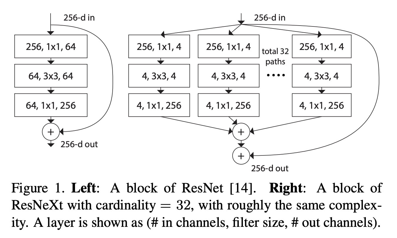
content_review(f"{feedback_prefix}_Improving_efficiency_Inception_and_ResNeXt_Video")

ResNetとResNeXtの比較

Xie et al., 2016

インタラクティブデモ 5: ResNet vs. ResNeXt

以下のウィジェットは、ResNet（上）とResNeXt（下）のパラメータ数を計算します。入力チャネル数と出力チャネル数（または特徴マップ数）は同じと仮定しています（ウィジェット内の「Channels in+out」と表示）。ResNetまたはResNeXtの1つのブロックの最初と2番目の層の後のチャネル数を「ボトルネックチャネル」と呼びます。

スライダーは現在、上の図に示されている位置にあります。以下の課題の目的は、ResNetとResNeXtの表現力とパラメータ数の違いを調査することです。

# @title Parameter Calculator
# @markdown Run this cell to enable the widget
from IPython.display import display as dis

def calculate_parameters_resnet(d_in, resnet_channels):
    """
    ResNet math: Implement how parameters scale

    Args:
      d_in: int
        Input dimensionality
      resnet_channels: int
        Number of channels in ResNet

    Returns:
      None
    """
    d_out = d_in
    resnet_parameters = d_in*resnet_channels + 3*3*resnet_channels*resnet_channels + resnet_channels*d_out

    print('ResNet parameters: {}'.format(resnet_parameters))
    return None


def calculate_parameters_resnext(d_in, resnext_channels,
                                 num_paths):
    """
    ResNext math: Implement how parameters scale

    Args:
      d_in: int
        Input dimensionality
      resnet_channels: int
        Number of channels in ResNext
      num_paths: int
        Number of pathways in ResNext

    Returns:
      None
    """
    d_out = d_in
    d = resnext_channels

    resnext_parameters = (d_in*d + 3*3*d*d + d*d_out)*num_paths

    print('ResNeXt parameters: {}'.format(resnext_parameters))
    return None


labels = ['ResNet', 'ResNeXt']
descriptions_resnet = ['Channels in+out', 'Bottleneck channels']
descriptions_resnext = ['Channels in+out', 'Bottleneck channels',
                        'Number of paths (cardinality)']
lbox_resnet = widgets.VBox([widgets.Label(description) for description in descriptions_resnet])
lbox_resnext = widgets.VBox([widgets.Label(description) for description in descriptions_resnext])

d_in = widgets.FloatLogSlider(
    value=256,
    base=2,
    min=1, # Max exponent of base
    max=10, # Min exponent of base
    step=1, # Exponent step
)
resnet_channels = widgets.FloatLogSlider(
    value=64,
    base=2,
    min=5, # Max exponent of base
    max=10, # Min exponent of base
    step=1, # Exponent step
)
resnext_channels = widgets.FloatLogSlider(
    value=4,
    base=2,
    min=1, # Max exponent of base
    max=10, # Min exponent of base
    step=1, # Exponent step
)
num_paths = widgets.FloatLogSlider(
    value=32,
    base=2,
    min=0, # Max exponent of base
    max=7, # Min exponent of base
    step=1, # Exponent step
)

rbox_resnet = widgets.VBox([d_in, resnet_channels])
rbox_resnext = widgets.VBox([d_in, resnext_channels, num_paths])
ui_resnet = widgets.HBox([lbox_resnet, rbox_resnet])
ui_resnet_labeled = widgets.VBox(
    [widgets.HTML(value="<b>" + labels[0] + "</b>"), ui_resnet],
    layout=widgets.Layout(border='1px solid black'))
ui_resnext = widgets.HBox([lbox_resnext, rbox_resnext])
ui_resnext_labeled = widgets.VBox(
    [widgets.HTML(value="<b>" + labels[1] + "</b>"), ui_resnext],
    layout=widgets.Layout(border='1px solid black'))
ui = widgets.VBox([ui_resnet_labeled, ui_resnext_labeled])

out_resnet = widgets.interactive_output(calculate_parameters_resnet,
                     {'d_in':d_in,
                     'resnet_channels':resnet_channels})

out_resnext = widgets.interactive_output(calculate_parameters_resnext,
                     {'d_in':d_in,
                     'resnext_channels':resnext_channels,
                     'num_paths':num_paths})

d1 = dis(ui, out_resnet, out_resnext)

# @title Submit your feedback
content_review(f"{feedback_prefix}_ResNet_vs_ResNeXt_Interactive_Demo")

考えてみよう！ 5: ResNet vs. ResNeXt

上の図では、両方のネットワーク、すなわちResNetとResNeXtは、ほぼ同じパラメータ数を持っています。

1. それぞれのネットワークのボトルネックには何チャネルありますか？
2. それぞれのネットワークのブロック内で、最初の層から2番目の層へこれらのチャネルはどのように接続されていますか？
3. これらのことは、両モデルの表現力に対してどのような意味を持ちますか？

解答を見る$

# @title Submit your feedback
content_review(f"{feedback_prefix}_ResNet_vs_ResNeXt_Discussion")

次にパラメータ数を見てみましょう。

• ResNetとResNeXtの両方のボトルネックチャネル数を64に固定し、ResNeXtのパス数を変化させると、パラメータ数の差はどのように変わりますか？（例えば、8パスで各パスが8チャネルの場合など）
• どのパス数が最もパラメータの節約につながりますか？

解答を見る$

セクション 6: Depthwise Separable Convolutions（深さ方向分離畳み込み）

所要時間の目安: 約23分

# @title Video 6: Improving efficiency: MobileNet
from ipywidgets import widgets
from IPython.display import YouTubeVideo
from IPython.display import IFrame
from IPython.display import display


class PlayVideo(IFrame):
  def __init__(self, id, source, page=1, width=400, height=300, **kwargs):
    self.id = id
    if source == 'Bilibili':
      src = f'https://player.bilibili.com/player.html?bvid={id}&page={page}'
    elif source == 'Osf':
      src = f'https://mfr.ca-1.osf.io/render?url=https://osf.io/download/{id}/?direct%26mode=render'
    super(PlayVideo, self).__init__(src, width, height, **kwargs)


def display_videos(video_ids, W=400, H=300, fs=1):
  tab_contents = []
  for i, video_id in enumerate(video_ids):
    out = widgets.Output()
    with out:
      if video_ids[i][0] == 'Youtube':
        video = YouTubeVideo(id=video_ids[i][1], width=W,
                             height=H, fs=fs, rel=0)
        print(f'Video available at https://youtube.com/watch?v={video.id}')
      else:
        video = PlayVideo(id=video_ids[i][1], source=video_ids[i][0], width=W,
                          height=H, fs=fs, autoplay=False)
        if video_ids[i][0] == 'Bilibili':
          print(f'Video available at https://www.bilibili.com/video/{video.id}')
        elif video_ids[i][0] == 'Osf':
          print(f'Video available at https://osf.io/{video.id}')
      display(video)
    tab_contents.append(out)
  return tab_contents


video_ids = [('Youtube', 'kdbGpn1JfmU'), ('Bilibili', 'BV1D44y127fS')]
tab_contents = display_videos(video_ids, W=854, H=480)
tabs = widgets.Tab()
tabs.children = tab_contents
for i in range(len(tab_contents)):
  tabs.set_title(i, video_ids[i][0])
display(tabs)

# @title Submit your feedback
content_review(f"{feedback_prefix}_Improving_efficiency_MobileNet_Video")

セクション 6.1: Depthwise Separable Convolutions（深さ方向分離畳み込み）

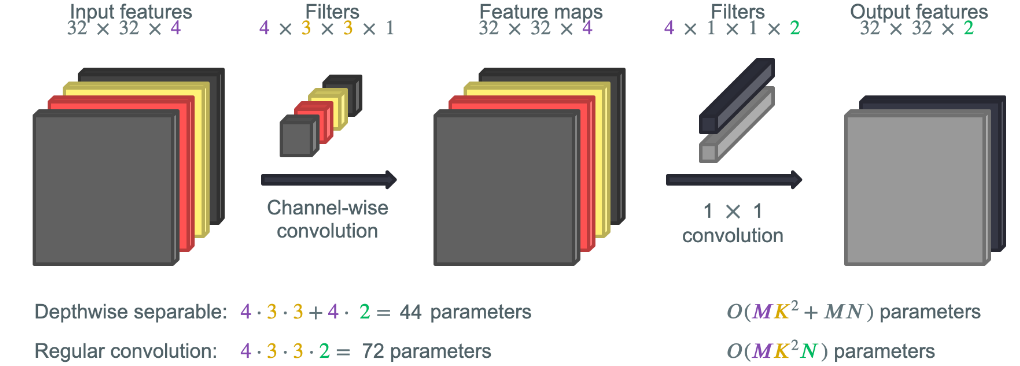
大規模モデルの計算コストを削減するもう一つの方法は、depthwise separable convolutions（深さ方向分離畳み込み）の利用です（こちらで紹介$）。深さ方向分離畳み込みは、MobileNetsを効率的にしている重要な要素です。

コーディング演習 6.1: パラメータ数の計算

以下の関数内で、通常の畳み込みと深さ方向分離畳み込みのパラメータ数の計算を完成させてください。
上の動画で示された例を参考に、計算が正しいか確認できます。

def convolution_math(in_channels, filter_size, out_channels):
  """
  Convolution math: Implement how parameters scale as a function of feature maps
  and filter size in convolution vs depthwise separable convolution.

  Args:
    in_channels : int
      Number of input channels
    filter_size : int
      Size of the filter
    out_channels : int
      Number of output channels

  Returns:
    None
  """
  ####################################################################
  # Fill in all missing code below (...),
  # then remove or comment the line below to test your function
  raise NotImplementedError("Convolution math")
  ####################################################################
  # Calculate the number of parameters for regular convolution
  conv_parameters = ...
  # Calculate the number of parameters for depthwise separable convolution
  depthwise_conv_parameters = ...

  print(f"Depthwise separable: {depthwise_conv_parameters} parameters")
  print(f"Regular convolution: {conv_parameters} parameters")

  return None



## Uncomment to test your function
# convolution_math(in_channels=4, filter_size=3, out_channels=2)

Depthwise separable: 44 parameters
Regular convolution: 72 parameters

解答を見る$

# @title Submit your feedback
content_review(f"{feedback_prefix}_Calculation_of_parameters_Exercise")

考えてみよう！ 6.1: パラメータ節約は入力特徴マップ数（4 vs. 64）にどう依存するか？

解答を見る$

# @title Submit your feedback
content_review(f"{feedback_prefix}_Parameter_savings_Discussion")

セクション 7: 転移学習（Transfer Learning）

所要時間の目安: 約24分

# @title Video 7: Transfer Learning
from ipywidgets import widgets
from IPython.display import YouTubeVideo
from IPython.display import IFrame
from IPython.display import display


class PlayVideo(IFrame):
  def __init__(self, id, source, page=1, width=400, height=300, **kwargs):
    self.id = id
    if source == 'Bilibili':
      src = f'https://player.bilibili.com/player.html?bvid={id}&page={page}'
    elif source == 'Osf':
      src = f'https://mfr.ca-1.osf.io/render?url=https://osf.io/download/{id}/?direct%26mode=render'
    super(PlayVideo, self).__init__(src, width, height, **kwargs)


def display_videos(video_ids, W=400, H=300, fs=1):
  tab_contents = []
  for i, video_id in enumerate(video_ids):
    out = widgets.Output()
    with out:
      if video_ids[i][0] == 'Youtube':
        video = YouTubeVideo(id=video_ids[i][1], width=W,
                             height=H, fs=fs, rel=0)
        print(f'Video available at https://youtube.com/watch?v={video.id}')
      else:
        video = PlayVideo(id=video_ids[i][1], source=video_ids[i][0], width=W,
                          height=H, fs=fs, autoplay=False)
        if video_ids[i][0] == 'Bilibili':
          print(f'Video available at https://www.bilibili.com/video/{video.id}')
        elif video_ids[i][0] == 'Osf':
          print(f'Video available at https://osf.io/{video.id}')
      display(video)
    tab_contents.append(out)
  return tab_contents


video_ids = [('Youtube', 'Qr5l-an5ac4'), ('Bilibili', 'BV1z54y1E714')]
tab_contents = display_videos(video_ids, W=854, H=480)
tabs = widgets.Tab()
tabs.children = tab_contents
for i in range(len(tab_contents)):
  tabs.set_title(i, video_ids[i][0])
display(tabs)

# @title Submit your feedback
content_review(f"{feedback_prefix}_Transfer_Learning_Video")

実際の大規模画像モデルの最も一般的な訓練方法は転移学習です。まずImageNetのような大規模分類データセットでネットワークを事前学習し、その後このネットワークの重みを初期値として使い、目的のタスクに対して微調整（"ファインチューニング"）を行います。

ネットワークを2回訓練するのは一見奇妙に思えますが、ターゲットデータセットでの学習が速くなり、しばしば「ゼロから」訓練するよりも性能が良くなります。また、ノイズに対する頑健性などの利点もあり、これは活発な研究対象となっています。

このセクションでは、ImageNetで訓練されたモデルを使い、ポケモンの分類を学習させることで転移学習を実演します。

セクション 7.1: データのダウンロードと準備

# @title Download Data
import zipfile, io

# Original link: https://github.com/ben-heil/cis_522_data.git
url = 'https://osf.io/u4njm/download'

fname = 'small_pokemon_dataset'

if not os.path.exists(fname+'zip'):
  print("Data is being downloaded...")
  r = requests.get(url, stream=True)
  z = zipfile.ZipFile(io.BytesIO(r.content))
  z.extractall()
  print("The download has been completed.")
else:
  print("Data has already been downloaded.")

# List the different Pokemon
os.listdir("small_pokemon_dataset/")

# @title Determine number of classes
num_classes = 0
for folders in os.listdir('small_pokemon_dataset/'):
  num_classes += 1
print(f"{num_classes} types of Pokemon")

# @title Display Example Images
train_transform = transforms.Compose((transforms.Resize((256, 256)),
                                      transforms.ToTensor()))

pokemon_dataset = ImageFolder('small_pokemon_dataset',
                              transform=train_transform)

image_count = len(pokemon_dataset)
train_indices = []
test_indices = []
for i in range(image_count):
  # Put ten percent of the images in the test set
  if random.random() < .1:
    test_indices.append(i)
  else:
    train_indices.append(i)

pokemon_test_set = torch.utils.data.Subset(pokemon_dataset, test_indices)
pokemon_train_set = torch.utils.data.Subset(pokemon_dataset, train_indices)

pokemon_train_loader = torch.utils.data.DataLoader(pokemon_train_set,
                                                   batch_size=16,
                                                   shuffle=True,)
pokemon_test_loader = torch.utils.data.DataLoader(pokemon_test_set,
                                                  batch_size=16)

dataiter = iter(pokemon_train_loader)
images, labels = next(dataiter)

# Show images
plt.imshow(make_grid(images, nrow=4).permute(1, 2, 0))
plt.axis('off')
plt.show()

セクション 7.2: ResNetのファインチューニング

コンピュータビジョンでは、大規模データセット（多くの場合ImageNet）で訓練された大きなモデルを取り、分類層を置き換え、ネットワーク全体を微調整して別のタスクを実行させることが一般的です。

ここでは、事前学習済みのResNetモデルを使ってポケモンのタイプを分類します。

resnet = torchvision.models.resnet18(weights='ResNet18_Weights.DEFAULT')
num_ftrs = resnet.fc.in_features
# Reset final fully connected layer, number of classes = types of Pokemon = 9
resnet.fc = nn.Linear(num_ftrs, num_classes)
resnet.to(DEVICE)
optimizer = torch.optim.Adam(resnet.parameters(), lr=1e-4)
loss_fn = nn.CrossEntropyLoss()

# @title Finetune ResNet
pretrained_accs = []
for epoch in tqdm.tqdm(range(10)):
  # Train loop
  for batch in pokemon_train_loader:
    images, labels = batch
    images = images.to(DEVICE)
    labels = labels.to(DEVICE)

    optimizer.zero_grad()
    output = resnet(images)
    loss = loss_fn(output, labels)
    loss.backward()
    optimizer.step()

  # Eval loop
  with torch.no_grad():
    loss_sum = 0
    total_correct = 0
    total = len(pokemon_test_set)
    for batch in pokemon_test_loader:
      images, labels = batch
      images = images.to(DEVICE)
      labels = labels.to(DEVICE)
      output = resnet(images)
      loss = loss_fn(output, labels)
      loss_sum += loss.item()

      predictions = torch.argmax(output, dim=1)

      num_correct = torch.sum(predictions == labels)
      total_correct += num_correct

    # Plot accuracy
    pretrained_accs.append(total_correct.cpu() / total)
    plt.plot(pretrained_accs)
    plt.xlabel('epoch')
    plt.ylabel('accuracy')
    plt.title('Pokemon prediction accuracy')
    IPython.display.clear_output(wait=True)
    IPython.display.display(plt.gcf())
  plt.close()

セクション 7.3: 分類層のみの訓練

転移学習の別の方法として、事前学習済みモデルの最後の層（分類層、時に「線形リードアウト」とも呼ばれる）だけを置き換えます。前述のようにネットワーク全体を微調整する代わりに、分類層のみを訓練します。

resnet = torchvision.models.resnet18(weights='ResNet18_Weights.DEFAULT')
for param in resnet.parameters():
  param.requires_grad = False
num_ftrs = resnet.fc.in_features
# ResNet final fully connected layer
resnet.fc = nn.Linear(num_ftrs, num_classes)
resnet.to(DEVICE)
optimizer = torch.optim.Adam(resnet.fc.parameters(), lr=1e-2)
loss_fn = nn.CrossEntropyLoss()

# @title Finetune readout of ResNet
linreadout_accs = []
for epoch in tqdm.tqdm(range(10)):
  # Train loop
  for batch in pokemon_train_loader:
    images, labels = batch
    images = images.to(DEVICE)
    labels = labels.to(DEVICE)

    optimizer.zero_grad()
    output = resnet(images)
    loss = loss_fn(output, labels)
    loss.backward()
    optimizer.step()

  # Eval loop
  with torch.no_grad():
    loss_sum = 0
    total_correct = 0
    total = len(pokemon_test_set)
    for batch in pokemon_test_loader:
      images, labels = batch
      images = images.to(DEVICE)
      labels = labels.to(DEVICE)
      output = resnet(images)
      loss = loss_fn(output, labels)
      loss_sum += loss.item()

      predictions = torch.argmax(output, dim=1)

      num_correct = torch.sum(predictions == labels)
      total_correct += num_correct

    # Plot accuracy
    linreadout_accs.append(total_correct.cpu() / total)
    plt.plot(linreadout_accs)
    plt.xlabel('epoch')
    plt.ylabel('accuracy')
    plt.title('Pokemon prediction accuracy')
    IPython.display.clear_output(wait=True)
    IPython.display.display(plt.gcf())
  plt.close()

セクション 7.4: ResNetをゼロから訓練

比較のためのベースラインとして、ResNetを「ゼロから」訓練します。つまり、重みをランダムに初期化し、ポケモンデータセットだけでネットワーク全体を訓練します。

resnet = torchvision.models.resnet18(weights=None)
num_ftrs = resnet.fc.in_features
# ResNet final fully connected layer
resnet.fc = nn.Linear(num_ftrs, num_classes)
resnet.to(DEVICE)
optimizer = torch.optim.Adam(resnet.parameters(), lr=1e-4)

loss_fn = nn.CrossEntropyLoss()

# @title Train ResNet from scratch
scratch_accs = []
for epoch in tqdm.tqdm(range(10)):
  # Train loop
  for batch in pokemon_train_loader:
    images, labels = batch
    images = images.to(DEVICE)
    labels = labels.to(DEVICE)

    optimizer.zero_grad()
    output = resnet(images)
    loss = loss_fn(output, labels)
    loss.backward()
    optimizer.step()

  # Eval loop
  with torch.no_grad():
    loss_sum = 0
    total_correct = 0
    total = len(pokemon_test_set)
    for batch in pokemon_test_loader:
      images, labels = batch
      images = images.to(DEVICE)
      labels = labels.to(DEVICE)
      output = resnet(images)
      loss = loss_fn(output, labels)
      loss_sum += loss.item()

      predictions = torch.argmax(output, dim=1)

      num_correct = torch.sum(predictions == labels)
      total_correct += num_correct

    scratch_accs.append(total_correct.cpu() / total)
    plt.plot(scratch_accs)
    plt.xlabel('epoch')
    plt.ylabel('accuracy')
    plt.title('Pokemon prediction accuracy')

    IPython.display.clear_output(wait=True)
    IPython.display.display(plt.gcf())
  plt.close()

セクション 7.5: 直接比較

ランダム初期化のネットワークは特に小規模データセットの場合、性能が劣ります。モデルの収束が遅く、均一でないことに注意してください。

# @title Plot Accuracies
plt.plot(pretrained_accs, label='Pretrained: fine-tuning')
plt.plot(linreadout_accs, label='Pretrained: linear Readout')
plt.plot(scratch_accs, label='Trained from Scratch')
plt.title('Pokemon prediction accuracy')
plt.legend()
plt.show()

演習 7.5.1: 事前学習済みResNet vs. ゼロから訓練したResNet

まず、事前学習済みResNetとゼロから訓練したResNetを比較します。なぜ事前学習済みモデルはゼロから訓練したモデルより優れることがあるのでしょうか？どんな場合に劣ると予想されますか？

解答を見る$

# @title Submit your feedback
content_review(f"{feedback_prefix}_Pretrained_ResNet_vs_ResNet_Exercise")

演習 7.5.2: 分類層のみの訓練

次に、転移学習の異なる方法、すなわちネットワーク全体の微調整と分類層のみの訓練を見てみましょう。なぜネットワーク全体の微調整が分類層のみの訓練より優れることがあるのでしょうか？分類層のみの訓練の利点は何でしょう？どんな場合に両者の性能が似ると予想されますか？

解答を見る$

# @title Submit your feedback
content_review(f"{feedback_prefix}_Training_only_the_classification_Exercise")

さらなる参考文献

ここで見たような教師あり事前学習は有用ですが、外部データを利用してモデルを改善する他の方法もあります。特に現在人気なのはコントラスト学習のような自己教師あり学習技術です。

また、モデルサイズ、事前学習データセットサイズ、訓練データセットサイズ、性能の関係を定量化しようとする最近の論文もあります。

まとめ

このチュートリアルでは、モダンな畳み込みニューラルネットワーク（CNN）の構造と動作原理について学びました。また、転移学習の概念に慣れ、いつ適用すべきかを理解しました。時間があれば、速度と精度のトレードオフについても学びます。次のチュートリアルでは、顔認識タスクにおけるモダンな畳み込みネットワークを見ていきます。

# @title Video 8: Summary and Outlook
from ipywidgets import widgets
from IPython.display import YouTubeVideo
from IPython.display import IFrame
from IPython.display import display


class PlayVideo(IFrame):
  def __init__(self, id, source, page=1, width=400, height=300, **kwargs):
    self.id = id
    if source == 'Bilibili':
      src = f'https://player.bilibili.com/player.html?bvid={id}&page={page}'
    elif source == 'Osf':
      src = f'https://mfr.ca-1.osf.io/render?url=https://osf.io/download/{id}/?direct%26mode=render'
    super(PlayVideo, self).__init__(src, width, height, **kwargs)


def display_videos(video_ids, W=400, H=300, fs=1):
  tab_contents = []
  for i, video_id in enumerate(video_ids):
    out = widgets.Output()
    with out:
      if video_ids[i][0] == 'Youtube':
        video = YouTubeVideo(id=video_ids[i][1], width=W,
                             height=H, fs=fs, rel=0)
        print(f'Video available at https://youtube.com/watch?v={video.id}')
      else:
        video = PlayVideo(id=video_ids[i][1], source=video_ids[i][0], width=W,
                          height=H, fs=fs, autoplay=False)
        if video_ids[i][0] == 'Bilibili':
          print(f'Video available at https://www.bilibili.com/video/{video.id}')
        elif video_ids[i][0] == 'Osf':
          print(f'Video available at https://osf.io/{video.id}')
      display(video)
    tab_contents.append(out)
  return tab_contents


video_ids = [('Youtube', 'sjj0-7i6XfE'), ('Bilibili', 'BV1So4y1D7Ev')]
tab_contents = display_videos(video_ids, W=854, H=480)
tabs = widgets.Tab()
tabs.children = tab_contents
for i in range(len(tab_contents)):
  tabs.set_title(i, video_ids[i][0])
display(tabs)

# @title Submit your feedback
content_review(f"{feedback_prefix}_Summary_and_Outlook_Video")

ボーナス: 速度-精度トレードオフ / 異なるバックボーン

所要時間の目安: 約21分

# @title Video 9: Speed-accuracy trade-off
from ipywidgets import widgets
from IPython.display import YouTubeVideo
from IPython.display import IFrame
from IPython.display import display


class PlayVideo(IFrame):
  def __init__(self, id, source, page=1, width=400, height=300, **kwargs):
    self.id = id
    if source == 'Bilibili':
      src = f'https://player.bilibili.com/player.html?bvid={id}&page={page}'
    elif source == 'Osf':
      src = f'https://mfr.ca-1.osf.io/render?url=https://osf.io/download/{id}/?direct%26mode=render'
    super(PlayVideo, self).__init__(src, width, height, **kwargs)


def display_videos(video_ids, W=400, H=300, fs=1):
  tab_contents = []
  for i, video_id in enumerate(video_ids):
    out = widgets.Output()
    with out:
      if video_ids[i][0] == 'Youtube':
        video = YouTubeVideo(id=video_ids[i][1], width=W,
                             height=H, fs=fs, rel=0)
        print(f'Video available at https://youtube.com/watch?v={video.id}')
      else:
        video = PlayVideo(id=video_ids[i][1], source=video_ids[i][0], width=W,
                          height=H, fs=fs, autoplay=False)
        if video_ids[i][0] == 'Bilibili':
          print(f'Video available at https://www.bilibili.com/video/{video.id}')
        elif video_ids[i][0] == 'Osf':
          print(f'Video available at https://osf.io/{video.id}')
      display(video)
    tab_contents.append(out)
  return tab_contents


video_ids = [('Youtube', '9p4gD-QnbIQ'), ('Bilibili', 'BV1v64y1z7PT')]
tab_contents = display_videos(video_ids, W=854, H=480)
tabs = widgets.Tab()
tabs.children = tab_contents
for i in range(len(tab_contents)):
  tabs.set_title(i, video_ids[i][0])
display(tabs)

# @title Submit your feedback
content_review(f"{feedback_prefix}_SpeedAccuracy_TradeOff_Different_Backbones_Bonus_Video")

モデルが大きくなり接続数が増えるにつれて、計算コストも増大しました。現代の画像処理では、モデル性能と計算コストのトレードオフがあります。多くの問題でモデルは非常に高い性能を達成できますが、最先端の結果を得るには膨大な計算資源が必要です。

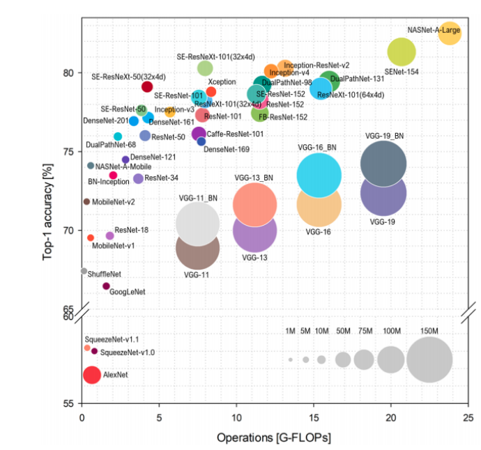
ボーナスコーディング演習: 異なるモデルの精度と訓練速度の比較

目標は3つの事前学習済みモデルを読み込み、ファインチューニングすることです。
modelsはモデル名をキー、対応するモデルオブジェクトを値とする辞書です。
現在のモデル名はResNet18, AlexNet, VGG-19です。
まずはtorchvision.modelsからこれらのモデルを読み込み、事前学習済みであることを確認してください。

他のモデルを試したい場合は、辞書を変更するか、3つ以上試したい場合は辞書に追加し、以下の配列に学習率を追加してください。

# @title Imagenette Train Loop: `train_loop(model, optimizer, train_loader, loss_fn, device)`
def train_loop(model, optimizer, train_loader,
               loss_fn, device):
  """
  Imagenette Train Loop

  Args:
    model: nn.module
      Model
    optimizer: function
      Optimizer
    train_loader: torch.loader
      Training dataset
    loss_fn: function
      Criterion
    device: string
      GPU/CUDA if available. CPU otherwise.

  Returns:
    Average Training time
  """
  times = []
  model.to(device)
  for epoch in tqdm.tqdm(range(5)):
    model.train()
    t_start = time.time()

    # Train on a batch of images
    for imagenette_batch in train_loader:
      images, labels = imagenette_batch

      # Convert labels from imagenette indices to imagenet labels
      for i, label in enumerate(labels):
        labels[i] = dir_index_to_imagenet_label[label.item()]

      images = images.to(device)
      labels = labels.to(device)
      output = model(images)
      optimizer.zero_grad()
      loss = loss_fn(output, labels)
      loss.backward()
      optimizer.step()
      if torch.cuda.is_available():
        torch.cuda.synchronize()

      times += [time.time() - t_start]

  return np.mean(times)

# @title Run the models: `run_models(models, lr_rates)`
def run_models(models, lr_rates):
  """
  Run the models

  Args:
    models: dict
      Models
    lr_rates: list
      Learning rates

  Returns:
    times: list
      Running time for models
    top_1_acciracies: list
      Top 1 accuracy per model
  """
  times, top_1_accuracies = [], []

  for (name, model), lr in zip(models.items(), lr_rates):

    print(name, lr)

    model.to(DEVICE)
    model.aux_logits = False  # Important only for googlenet

    optimizer = torch.optim.Adam(model.parameters(), lr=lr)
    loss_fn = nn.CrossEntropyLoss()

    model_time = train_loop(model, optimizer, imagenette_train_loader, loss_fn,
                            DEVICE)
    times.append(model_time)

    top_1_acc, _ = eval_imagenette(model, imagenette_val_loader,
                                  len(imagenette_val), device=DEVICE)
    top_1_accuracies.append(top_1_acc.item())

  return times, top_1_accuracies

# @title Plot accuracies vs. training speed
def get_parameter_count(model):
  """
  Get parameter count per model

  Args:
    model: nn.module
      Model

  Returns:
    Parameter count for model
  """
  return sum([torch.numel(p) for p in model.parameters()])


def plot_acc_speed(times, accs, models):
  """
  Plots Accuracy vs Speed

  Args:
    times: list
      Log of running times
    accs: list
      Log of accuracies
    models: dict
      Log of models

  Returns:
    Nothing
  """
  ti = [t*1000 for t in times]
  for i, model in enumerate(list(models.keys())):
    scale = get_parameter_count(models[model])*1e-6
    plt.scatter(ti[i], accs[i], s=scale, label=model)
  plt.grid(True)
  plt.xlabel('Speed [ms]')
  plt.ylabel('Accuracy')
  plt.title('Accuracy vs. Speed')
  plt.legend()

def create_models(weights):
  """
  Creates models

  Args:
    weights: list of strings
      If True, load pretrained models.

  Returns:
    models: dict
      Log of models
    lr_rates: list
      Log of learning rates
  """
  ####################################################################
  # Fill in all missing code below (...),
  # then remove or comment the line below to test your function
  raise NotImplementedError("create pretrained models")
  ####################################################################
  # Load three pretrained models from torchvision.models
  # [these are just examples, other models are possible as well]
  model1 = ...
  model2 = ...
  model3 = ...

  models = {'...': model1, '...': model2, '...': model3}
  lr_rates = [1e-4, 1e-4, 1e-4]

  return models, lr_rates


weight_list = ['ResNet18_Weights.DEFAULT', 'AlexNet_Weights.DEFAULT', 'VGG19_Weights.DEFAULT']
## Uncomment below to test your function
# models, lr_rates = create_models(weights=weight_list)
# times, top_1_accuracies = run_models(models, lr_rates)
# plot_acc_speed(times, top_1_accuracies, models)

解答を見る$

出力例:

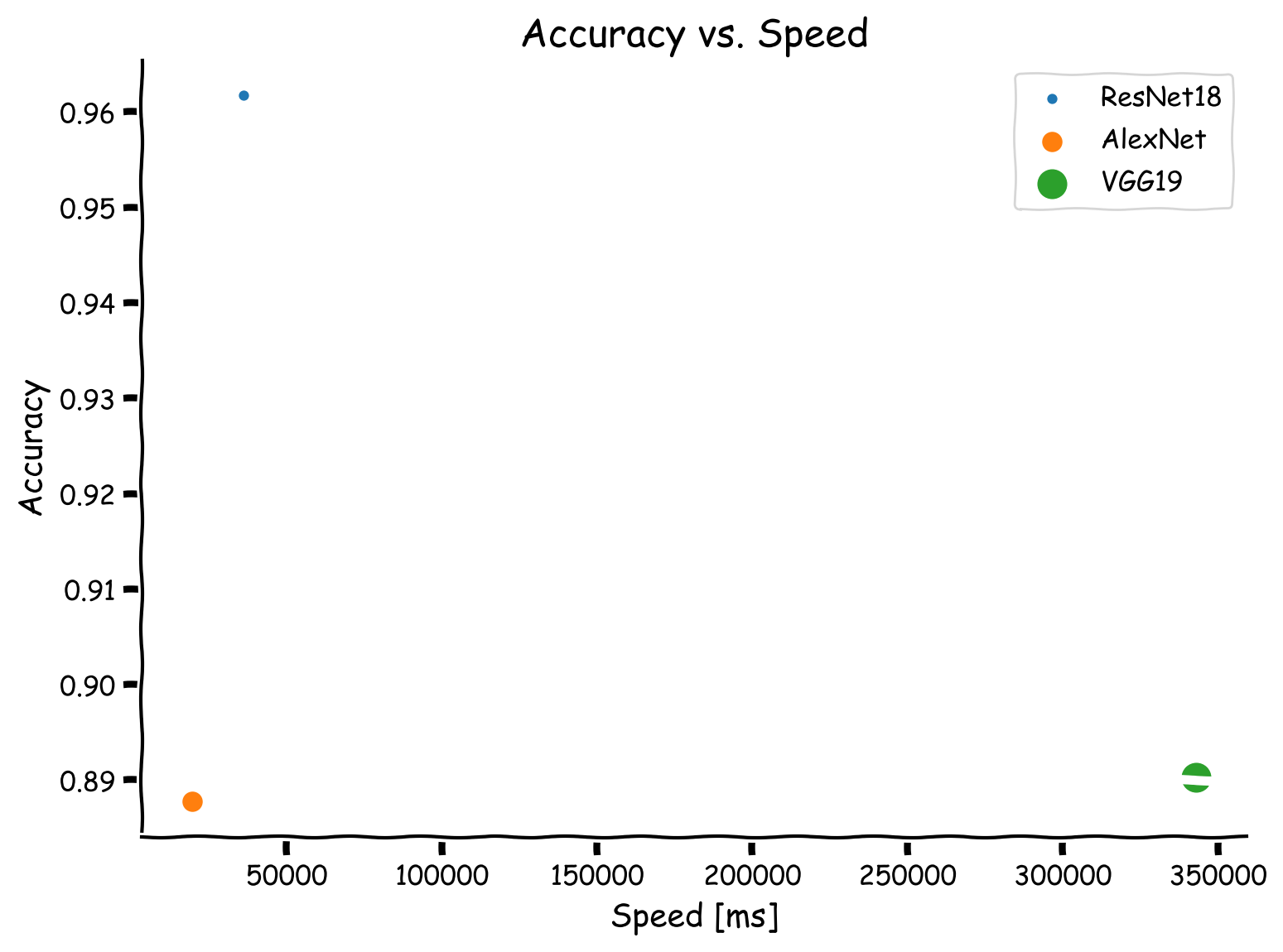
# @title Submit your feedback
content_review(f"{feedback_prefix}_Accuracy_vs_Training_Speed_Exercise")

ボーナス演習 1: 最適なモデルの選択

上のプロットを見てください。
これは選択したモデルの訓練速度と精度を示しています。
訓練速度は1エポックあたりの平均訓練時間で測定されています。
マーカーの大きさはモデルのパラメータ数を表しています。

このタスクに最適なモデルはどれだと思いますか？なぜそう思いますか？
速度、精度、パラメータ数に基づいて結論を説明してください。

解答を見る$

# @title Submit your feedback
content_review(f"{feedback_prefix}_Finding_best_model_Exercise")

ボーナス演習 2: 速度と精度の相関

速度は精度とどのように相関していますか？速いモデルはより精度が高いですか？

解答を見る$

# @title Submit your feedback
content_review(f"{feedback_prefix}_Speed_and_accuracy_correlation_Exercise")