![]()

チュートリアル 1: CNNの紹介
第2週、第2日目:畳み込みネットワークと深層学習の考え方
Neuromatch Academyによる
コンテンツ作成者: Dawn Estes McKnight, Richard Gerum, Cassidy Pirlot, Rohan Saha, Liam Peet-Pare, Saeed Najafi, Alona Fyshe
コンテンツレビュアー: Saeed Salehi, Lily Cheng, Yu-Fang Yang, Polina Turishcheva, Bettina Hein, Kelson Shilling-Scrivo
コンテンツ編集者: Gagana B, Nina Kudryashova, Anmol Gupta, Xiaoxiong Lin, Spiros Chavlis
制作編集者: Alex Tran-Van-Minh, Gagana B, Spiros Chavlis
以下の資料を基にしています: Konrad Kording, Hmrishav Bandyopadhyay, Rahul Shekhar, Tejas Srivastava
チュートリアルの目標
このチュートリアルの終わりには、以下ができるようになります:
- 畳み込みとは何かを定義できる
- 畳み込みを演算として実装できる
このチュートリアルのボーナスマテリアルでは、以下もできるようになります:
- 自分でトレインループを書いてCNNを訓練する
- 過学習の兆候を認識し、それを改善する方法を理解する
# @title Tutorial slides
from IPython.display import IFrame
link_id = "s8xz5"
print(f"If you want to download the slides: https://osf.io/download/{link_id}/")
IFrame(src=f"https://mfr.ca-1.osf.io/render?url=https://osf.io/{link_id}/?direct%26mode=render%26action=download%26mode=render", width=854, height=480)
セットアップ
# @title Install dependencies# @title Install and import feedback gadget
from vibecheck import DatatopsContentReviewContainer
def content_review(notebook_section: str):
return DatatopsContentReviewContainer(
"", # No text prompt
notebook_section,
{
"url": "https://pmyvdlilci.execute-api.us-east-1.amazonaws.com/klab",
"name": "neuromatch_dl",
"user_key": "f379rz8y",
},
).render()
feedback_prefix = "W2D2_T1"# Imports
import time
import torch
import scipy.signal
import numpy as np
import matplotlib.pyplot as plt
import torch.nn as nn
import torch.nn.functional as F
import torchvision.transforms as transforms
import torchvision.datasets as datasets
from torch.utils.data import DataLoader
from tqdm.notebook import tqdm, trange
from PIL import Image# @title Figure Settings
import logging
logging.getLogger('matplotlib.font_manager').disabled = True
import ipywidgets as widgets # Interactive display
%matplotlib inline
%config InlineBackend.figure_format = 'retina'
plt.style.use("https://raw.githubusercontent.com/NeuromatchAcademy/content-creation/main/nma.mplstyle")# @title Helper functions
from scipy.signal import correlate2d
import zipfile, gzip, shutil, tarfile
def download_data(fname, folder, url, tar):
"""
Data downloading from OSF.
Args:
fname : str
The name of the archive
folder : str
The name of the destination folder
url : str
The download url
tar : boolean
`tar=True` the archive is `fname`.tar.gz, `tar=False` is `fname`.zip
Returns:
Nothing.
"""
if not os.path.exists(folder):
print(f'\nDownloading {folder} dataset...')
r = requests.get(url, allow_redirects=True)
with open(fname, 'wb') as fh:
fh.write(r.content)
print(f'\nDownloading {folder} completed.')
print('\nExtracting the files...\n')
if not tar:
with zipfile.ZipFile(fname, 'r') as fz:
fz.extractall()
else:
with tarfile.open(fname) as ft:
ft.extractall()
# Remove the archive
os.remove(fname)
# Extract all .gz files
foldername = folder + '/raw/'
for filename in os.listdir(foldername):
# Remove the extension
fname = filename.replace('.gz', '')
# Gunzip all files
with gzip.open(foldername + filename, 'rb') as f_in:
with open(foldername + fname, 'wb') as f_out:
shutil.copyfileobj(f_in, f_out)
os.remove(foldername+filename)
else:
print(f'{folder} dataset has already been downloaded.\n')
def check_shape_function(func, image_shape, kernel_shape):
"""
Helper function to check shape implementation
Args:
func: f.__name__
Function name
image_shape: tuple
Image shape
kernel_shape: tuple
Kernel shape
Returns:
Nothing
"""
correct_shape = correlate2d(np.random.rand(*image_shape), np.random.rand(*kernel_shape), "valid").shape
user_shape = func(image_shape, kernel_shape)
if correct_shape != user_shape:
print(f"❌ Your calculated output shape is not correct.")
else:
print(f"✅ Output for image_shape: {image_shape} and kernel_shape: {kernel_shape}, output_shape: {user_shape}, is correct.")
def check_conv_function(func, image, kernel):
"""
Helper function to check conv_function
Args:
func: f.__name__
Function name
image: np.ndarray
Image matrix
kernel_shape: np.ndarray
Kernel matrix
Returns:
Nothing
"""
solution_user = func(image, kernel)
solution_scipy = correlate2d(image, kernel, "valid")
result_right = (solution_user == solution_scipy).all()
if result_right:
print("✅ The function calculated the convolution correctly.")
else:
print("❌ The function did not produce the right output.")
print("For the input matrix:")
print(image)
print("and the kernel:")
print(kernel)
print("the function returned:")
print(solution_user)
print("the correct output would be:")
print(solution_scipy)
def check_pooling_net(net, device='cpu'):
"""
Helper function to check pooling output
Args:
net: nn.module
Net instance
device: string
GPU/CUDA if available, CPU otherwise.
Returns:
Nothing
"""
x_img = emnist_train[x_img_idx][0].unsqueeze(dim=0).to(device)
output_x = net(x_img)
output_x = output_x.squeeze(dim=0).detach().cpu().numpy()
right_output = [
[0.000000, 0.000000, 0.000000, 0.000000, 0.000000, 0.000000, 0.000000,
0.000000, 0.000000, 0.000000, 0.000000, 0.000000],
[0.000000, 0.000000, 0.000000, 0.000000, 0.000000, 0.000000, 0.000000,
0.000000, 0.000000, 0.000000, 0.000000, 0.000000],
[9.309552, 1.6216984, 0.000000, 0.000000, 0.000000, 0.000000, 2.2708383,
2.6654134, 1.2271233, 0.000000, 0.000000, 0.000000],
[12.873457, 13.318945, 9.46229, 4.663746, 0.000000, 0.000000, 1.8889914,
0.31068993, 0.000000, 0.000000, 0.000000, 0.000000],
[0.000000, 8.354934, 10.378724, 16.882853, 18.499334, 4.8546696, 0.000000,
0.000000, 0.000000, 6.29296, 5.096506, 0.000000],
[0.000000, 0.000000, 0.31068993, 5.7074604, 9.984148, 4.12916, 8.10037,
7.667609, 0.000000, 0.000000, 1.2780352, 0.000000],
[0.000000, 2.436305, 3.9764223, 0.000000, 0.000000, 0.000000, 12.98801,
17.1756, 17.531992, 11.664275, 1.5453291, 0.000000],
[4.2691708, 2.3217516, 0.000000, 0.000000, 1.3798618, 0.05612564, 0.000000,
0.000000, 11.218788, 16.360992, 13.980816, 8.354935],
[1.8126211, 0.000000, 0.000000, 2.9199777, 3.9382377, 0.000000, 0.000000,
0.000000, 0.000000, 0.000000, 6.076582, 10.035061],
[0.000000, 0.92164516, 4.434638, 0.7816348, 0.000000, 0.000000, 0.000000,
0.000000, 0.000000, 0.000000, 0.000000, 0.83254766],
[0.000000, 0.000000, 0.000000, 0.000000, 0.000000, 0.000000, 0.000000,
0.000000, 0.000000, 0.000000, 0.000000, 0.000000],
[0.000000, 0.000000, 0.000000, 0.000000, 0.000000, 0.000000, 0.000000,
0.000000, 0.000000, 0.000000, 0.000000, 0.000000]
]
right_shape = (3, 12, 12)
if output_x.shape != right_shape:
print(f"❌ Your output does not have the right dimensions. Your output is {output_x.shape} the expected output is {right_shape}")
elif (output_x[0] != right_output).all():
print("❌ Your output is not right.")
else:
print("✅ Your network produced the correct output.")
# Just returns accuracy on test data
def test(model, device, data_loader):
"""
Test function
Args:
net: nn.module
Net instance
device: string
GPU/CUDA if available, CPU otherwise.
data_loader: torch.loader
Test loader
Returns:
acc: float
Test accuracy
"""
model.eval()
correct = 0
total = 0
for data in data_loader:
inputs, labels = data
inputs = inputs.to(device).float()
labels = labels.to(device).long()
outputs = model(inputs)
_, predicted = torch.max(outputs, 1)
total += labels.size(0)
correct += (predicted == labels).sum().item()
acc = 100 * correct / total
return f"{acc}%"# @title Plotting Functions
def display_image_from_greyscale_array(matrix, title):
"""
Display image from greyscale array
Args:
matrix: np.ndarray
Image
title: string
Title of plot
Returns:
Nothing
"""
_matrix = matrix.astype(np.uint8)
_img = Image.fromarray(_matrix, 'L')
plt.figure(figsize=(3, 3))
plt.imshow(_img, cmap='gray', vmin=0, vmax=255) # Using 220 instead of 255 so the examples show up better
plt.title(title)
plt.axis('off')
def make_plots(original, actual_convolution, solution):
"""
Function to build original image/obtained solution and actual convolution
Args:
original: np.ndarray
Image
actual_convolution: np.ndarray
Expected convolution output
solution: np.ndarray
Obtained convolution output
Returns:
Nothing
"""
display_image_from_greyscale_array(original, "Original Image")
display_image_from_greyscale_array(actual_convolution, "Convolution result")
display_image_from_greyscale_array(solution, "Your solution")
def plot_loss_accuracy(train_loss, train_acc,
validation_loss, validation_acc):
"""
Code to plot loss and accuracy
Args:
train_loss: list
Log of training loss
validation_loss: list
Log of validation loss
train_acc: list
Log of training accuracy
validation_acc: list
Log of validation accuracy
Returns:
Nothing
"""
epochs = len(train_loss)
fig, (ax1, ax2) = plt.subplots(1, 2)
ax1.plot(list(range(epochs)), train_loss, label='Training Loss')
ax1.plot(list(range(epochs)), validation_loss, label='Validation Loss')
ax1.set_xlabel('Epochs')
ax1.set_ylabel('Loss')
ax1.set_title('Epoch vs Loss')
ax1.legend()
ax2.plot(list(range(epochs)), train_acc, label='Training Accuracy')
ax2.plot(list(range(epochs)), validation_acc, label='Validation Accuracy')
ax2.set_xlabel('Epochs')
ax2.set_ylabel('Accuracy')
ax2.set_title('Epoch vs Accuracy')
ax2.legend()
fig.set_size_inches(15.5, 5.5)# @title Set random seed
# @markdown Executing `set_seed(seed=seed)` you are setting the seed
# For DL its critical to set the random seed so that students can have a
# baseline to compare their results to expected results.
# Read more here: https://pytorch.org/docs/stable/notes/randomness.html
# Call `set_seed` function in the exercises to ensure reproducibility.
import random
import torch
def set_seed(seed=None, seed_torch=True):
"""
Function that controls randomness.
NumPy and random modules must be imported.
Args:
seed : Integer
A non-negative integer that defines the random state. Default is `None`.
seed_torch : Boolean
If `True` sets the random seed for pytorch tensors, so pytorch module
must be imported. Default is `True`.
Returns:
Nothing.
"""
if seed is None:
seed = np.random.choice(2 ** 32)
random.seed(seed)
np.random.seed(seed)
if seed_torch:
torch.manual_seed(seed)
torch.cuda.manual_seed_all(seed)
torch.cuda.manual_seed(seed)
torch.backends.cudnn.benchmark = False
torch.backends.cudnn.deterministic = True
print(f'Random seed {seed} has been set.')
# In case that `DataLoader` is used
def seed_worker(worker_id):
"""
DataLoader will reseed workers following randomness in
multi-process data loading algorithm.
Args:
worker_id: integer
ID of subprocess to seed. 0 means that
the data will be loaded in the main process
Refer: https://pytorch.org/docs/stable/data.html#data-loading-randomness for more details
Returns:
Nothing
"""
worker_seed = torch.initial_seed() % 2**32
np.random.seed(worker_seed)
random.seed(worker_seed)# @title Set device (GPU or CPU). Execute `set_device()`
# especially if torch modules used.
# Inform the user if the notebook uses GPU or CPU.
def set_device():
"""
Set the device. CUDA if available, CPU otherwise
Args:
None
Returns:
Nothing
"""
device = "cuda" if torch.cuda.is_available() else "cpu"
if device != "cuda":
print("WARNING: For this notebook to perform best, "
"if possible, in the menu under `Runtime` -> "
"`Change runtime type.` select `GPU` ")
else:
print("GPU is enabled in this notebook.")
return deviceSEED = 2021
set_seed(seed=SEED)
DEVICE = set_device()セクション0: 先週の経験の振り返り
所要時間の目安:約15分
先週は多くのことを学びました! 過剰パラメータ化されたANNは効率的な普遍近似器である一方、データを丸暗記してしまうこともあります。しかし、正則化はANNの汎化性能を向上させる助けになります。L1正則化、L2正則化、データ拡張、ドロップアウトなど、いくつかの正則化手法を紹介しました。
今日は、ANNの構造を賢く変更することで単純化する別の方法について話します。
# @title Video 1: Introduction to CNNs and RNNs
from ipywidgets import widgets
from IPython.display import YouTubeVideo
from IPython.display import IFrame
from IPython.display import display


class PlayVideo(IFrame):
  def __init__(self, id, source, page=1, width=400, height=300, **kwargs):
    self.id = id
    if source == 'Bilibili':
      src = f'https://player.bilibili.com/player.html?bvid={id}&page={page}'
    elif source == 'Osf':
      src = f'https://mfr.ca-1.osf.io/render?url=https://osf.io/download/{id}/?direct%26mode=render'
    super(PlayVideo, self).__init__(src, width, height, **kwargs)


def display_videos(video_ids, W=400, H=300, fs=1):
  tab_contents = []
  for i, video_id in enumerate(video_ids):
    out = widgets.Output()
    with out:
      if video_ids[i][0] == 'Youtube':
        video = YouTubeVideo(id=video_ids[i][1], width=W,
                             height=H, fs=fs, rel=0)
        print(f'Video available at https://youtube.com/watch?v={video.id}')
      else:
        video = PlayVideo(id=video_ids[i][1], source=video_ids[i][0], width=W,
                          height=H, fs=fs, autoplay=False)
        if video_ids[i][0] == 'Bilibili':
          print(f'Video available at https://www.bilibili.com/video/{video.id}')
        elif video_ids[i][0] == 'Osf':
          print(f'Video available at https://osf.io/{video.id}')
      display(video)
    tab_contents.append(out)
  return tab_contents


video_ids = [('Youtube', '5598K-hS89A'), ('Bilibili', 'BV1cL411p7rz')]
tab_contents = display_videos(video_ids, W=854, H=480)
tabs = widgets.Tab()
tabs.children = tab_contents
for i in range(len(tab_contents)):
  tabs.set_title(i, video_ids[i][0])
display(tabs)
# @title Submit your feedback
content_review(f"{feedback_prefix}_Introduction_to_CNNs_and_RNNs_Video")考えてみよう!0: 正則化と有効パラメータ数
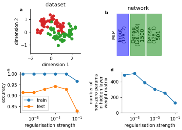
先週学んだ正則化について振り返りましょう。正則化にはいくつかの形態があります。例えば、L1正則化は損失関数に重みの絶対値の和に基づくペナルティ項を加えます。以下は、単純な1層の多層パーセプトロン(b)を単純なおもちゃデータセット(a)で訓練した結果です。
その下には、正則化が非ゼロ重みの数(d)とネットワークの精度(c)に与える影響を示す2つのグラフィックがあります。
何に気づきますか?
補足:Dense層は全結合層と同じです。PyTorchではこれをlinear層と呼びます。混乱しますが、これで理解できましたね!
# @title Submit your feedback
content_review(f"{feedback_prefix}_Regularization_and_effective_number_of_params_Discussion")
これからの内容
この後の講義では、パラメータ数を減らす別の方法、すなわち重み共有に焦点を当てます。重み共有とは、ある重みのセットをネットワークの複数の箇所で使い回すという考え方です。今日は主にCNNに注目し、画像の2次元空間にわたる重み共有について学びます。この空間にわたる重み共有はパラメータ数を減らし、ネットワークの汎化能力を高めます。類似のアプローチとして時系列にわたってパラメータを共有するリカレントニューラルネットワーク(RNN)がありますが、本チュートリアルでは扱いません。
セクション1: 神経科学的動機付けと一般的なCNN構造
所要時間の目安:約25分
# @title Video 2: Representations & Visual processing in the brain
from ipywidgets import widgets
from IPython.display import YouTubeVideo
from IPython.display import IFrame
from IPython.display import display


class PlayVideo(IFrame):
  def __init__(self, id, source, page=1, width=400, height=300, **kwargs):
    self.id = id
    if source == 'Bilibili':
      src = f'https://player.bilibili.com/player.html?bvid={id}&page={page}'
    elif source == 'Osf':
      src = f'https://mfr.ca-1.osf.io/render?url=https://osf.io/download/{id}/?direct%26mode=render'
    super(PlayVideo, self).__init__(src, width, height, **kwargs)


def display_videos(video_ids, W=400, H=300, fs=1):
  tab_contents = []
  for i, video_id in enumerate(video_ids):
    out = widgets.Output()
    with out:
      if video_ids[i][0] == 'Youtube':
        video = YouTubeVideo(id=video_ids[i][1], width=W,
                             height=H, fs=fs, rel=0)
        print(f'Video available at https://youtube.com/watch?v={video.id}')
      else:
        video = PlayVideo(id=video_ids[i][1], source=video_ids[i][0], width=W,
                          height=H, fs=fs, autoplay=False)
        if video_ids[i][0] == 'Bilibili':
          print(f'Video available at https://www.bilibili.com/video/{video.id}')
        elif video_ids[i][0] == 'Osf':
          print(f'Video available at https://osf.io/{video.id}')
      display(video)
    tab_contents.append(out)
  return tab_contents


video_ids = [('Youtube', 'AXO-iflKa58'), ('Bilibili', 'BV1c64y1x7mJ')]
tab_contents = display_videos(video_ids, W=854, H=480)
tabs = widgets.Tab()
tabs.children = tab_contents
for i in range(len(tab_contents)):
  tabs.set_title(i, video_ids[i][0])
display(tabs)
# @title Submit your feedback
content_review(f"{feedback_prefix}_Representations_and_Visual_processing_in_the_brain_Video")考えてみよう!1: 良い表現とは何か?
表現(representation)は長い歴史を持ち、紀元前300年のアリストテレスの時代から研究されてきました。表現は新しい概念ではなく、ニューラルネットワークだけに存在するものでもありません。
グループで、良い表現とは何か、そしてCNNを訓練するタスクによってそれがどう異なるかを話し合ってみてください。
時間があれば、脳の表現とニューラルネットワーク内の学習された表現がどう異なるかも考えてみてください。
# @title Submit your feedback
content_review(f"{feedback_prefix}_What_makes_a_representation_good_Discussion")
セクション2: 畳み込みとエッジ検出
所要時間の目安:約25分
CNNの基本は畳み込みです。なぜならCNNのCはConvolution(畳み込み)の頭文字だからです!このセクションでは、畳み込みとは何かを定義し、畳み込みを実際に行い、コードで実装します。
# @title Video 3: Details about Convolution
from ipywidgets import widgets
from IPython.display import YouTubeVideo
from IPython.display import IFrame
from IPython.display import display


class PlayVideo(IFrame):
  def __init__(self, id, source, page=1, width=400, height=300, **kwargs):
    self.id = id
    if source == 'Bilibili':
      src = f'https://player.bilibili.com/player.html?bvid={id}&page={page}'
    elif source == 'Osf':
      src = f'https://mfr.ca-1.osf.io/render?url=https://osf.io/download/{id}/?direct%26mode=render'
    super(PlayVideo, self).__init__(src, width, height, **kwargs)


def display_videos(video_ids, W=400, H=300, fs=1):
  tab_contents = []
  for i, video_id in enumerate(video_ids):
    out = widgets.Output()
    with out:
      if video_ids[i][0] == 'Youtube':
        video = YouTubeVideo(id=video_ids[i][1], width=W,
                             height=H, fs=fs, rel=0)
        print(f'Video available at https://youtube.com/watch?v={video.id}')
      else:
        video = PlayVideo(id=video_ids[i][1], source=video_ids[i][0], width=W,
                          height=H, fs=fs, autoplay=False)
        if video_ids[i][0] == 'Bilibili':
          print(f'Video available at https://www.bilibili.com/video/{video.id}')
        elif video_ids[i][0] == 'Osf':
          print(f'Video available at https://osf.io/{video.id}')
      display(video)
    tab_contents.append(out)
  return tab_contents


video_ids = [('Youtube', 'pmc40WCnF-w'), ('Bilibili', 'BV1Q64y1z77p')]
tab_contents = display_videos(video_ids, W=854, H=480)
tabs = widgets.Tab()
tabs.children = tab_contents
for i in range(len(tab_contents)):
  tabs.set_title(i, video_ids[i][0])
display(tabs)
# @title Submit your feedback
content_review(f"{feedback_prefix}_Details_about_convolution_Video")コーディング演習に入る前に、畳み込みの過程をステップごとに示したアニメーションを見てみましょう。
動画で見たように、畳み込みはカーネルを画像上でスライドさせ、要素ごとの積を取り、それらを合計する操作です。

A. Zhang, Z. C. Lipton, M. Li and A. J. Smola, Dive into Deep Learning$より引用。
注意: スライダーを動かすにはセルを実行し、スライダーを変えた後も再度実行する必要があります。
ヒント: このアニメーションや以降のものでは、赤線で下線が引かれたコード部分にマウスを乗せると値を変更できます。
ヒント: 下の関数名はConv2dとなっていますが、これは畳み込みフィルターが2次元の行列だからです。1次元や3次元の畳み込みもありますが、今日は扱いません。
インタラクティブデモ 2: 畳み込みの可視化
重要: デモを試すには、bool変数run_demoをチェックしてTrueにしてください。jupyter-bookの動画レンダリングの都合で自動実行からは外しています。
# @markdown *Run this cell to enable the widget!*

from IPython.display import HTML

id_html = 2
url = f'https://raw.githubusercontent.com/NeuromatchAcademy/course-content-dl/main/tutorials/W2D2_ConvnetsAndDlThinking/static/interactive_demo{id_html}.html'
run_demo = False  # @param {type:"boolean"}
if run_demo:
  display(HTML(url))
定義に関する注意
信号処理や数学の背景がある方は畳み込みを聞いたことがあるかもしれませんが、他分野の定義とここで使う定義は少し異なります。一般的な定義ではカーネルを水平方向と垂直方向に反転させてからスライドさせます。
ここでの目的では反転は不要です。もし反転を含む定義に慣れている場合は、カーネルがあらかじめ反転されていると考えてください。
一般的には、ここで畳み込みと呼んでいる反転なしの操作は_相関_(cross-correlation)として知られています(次の演習でscipy.signal.correlate2dを使う理由です)。初期の論文は一般的な畳み込み定義を使っていましたが、反転なしの方が視覚的にわかりやすく、CNNの学習能力には影響しません。
コーディング演習 2.1: 単純なカーネルの畳み込み
畳み込みは基本的に、_カーネル_または_フィルター_と呼ばれる小さな行列を、より大きな行列(ここでは画像のピクセル)に繰り返し掛け合わせる操作です。以下の画像とカーネルを考えます:
\begin{align}
&=
\begin{bmatrix}0 & 200 & 200 \0 & 0 & 200 \ 0 & 0 & 0
\end{bmatrix} \ \
&=
\begin{bmatrix} & \ & \frac{1}{4}
\end{bmatrix}
\end{align}
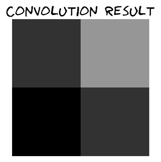
上記の画像とカーネルの畳み込みに必要な操作を手計算で行ってください。その後、以下のコードの「解答」セクションに結果を入力してください。このカーネルが元の画像に対して何をしているか考えてみましょう。
def conv_check():
  """
  Demonstration of convolution operation

  Args:
    None

  Returns:
    original: np.ndarray
      Image
    actual_convolution: np.ndarray
      Expected convolution output
    solution: np.ndarray
      Obtained convolution output
    kernel: np.ndarray
      Kernel
  """
  ####################################################################
  # Fill in missing code below (the elements of the matrix),
  # then remove or comment the line below to test your function
  raise NotImplementedError("Fill in the solution matrix, then delete this")
  ####################################################################
  # Write the solution array and call the function to verify it!
  solution = ...

  original = np.array([
                       [0, 200, 200],
                       [0, 0, 200],
                       [0, 0, 0]
                       ])

  kernel = np.array([
                     [0.25, 0.25],
                     [0.25, 0.25]
                     ])

  actual_convolution = scipy.signal.correlate2d(original, kernel, mode="valid")

  if (solution == actual_convolution).all():
    print("✅ Your solution is correct!\n")
  else:
    print("❌ Your solution is incorrect.\n")

  return original, kernel, actual_convolution, solution


## Uncomment to test your solution!
# original, kernel, actual_convolution, solution = conv_check()
# make_plots(original, actual_convolution, solution)例の出力:


# @title Submit your feedback
content_review(f"{feedback_prefix}_Convolution_of_a_simple_kernel_Exercise")
コーディング演習 2.2: 畳み込みの出力サイズ
手計算で畳み込みをしました。出力の形状はどう変わりましたか?入力行列とカーネルの形状が分かっているとき、出力の形状はどうなりますか?
ヒント: 出力の形状がわからない場合は、可視化に戻って画像やカーネルのサイズを変えたときの出力形状の変化を確認してください。
def calculate_output_shape(image_shape, kernel_shape):
  """
  Helper function to calculate output shape

  Args:
    image_shape: tuple
      Image shape
    kernel_shape: tuple
      Kernel shape

  Returns:
    output_height: int
      Output Height
    output_width: int
      Output Width
  """
  image_height, image_width = image_shape
  kernel_height, kernel_width = kernel_shape
  ####################################################################
  # Fill in missing code below, then remove or comment the line below to test your function
  raise NotImplementedError("Fill in the lines below, then delete this")
  ####################################################################
  output_height = ...
  output_width = ...
  return output_height, output_width


# Here we check if your function works correcly by applying it to different image
# and kernel shapes
# check_shape_function(calculate_output_shape, image_shape=(3, 3), kernel_shape=(2, 2))
# check_shape_function(calculate_output_shape, image_shape=(3, 4), kernel_shape=(2, 3))
# check_shape_function(calculate_output_shape, image_shape=(5, 5), kernel_shape=(5, 5))
# check_shape_function(calculate_output_shape, image_shape=(10, 20), kernel_shape=(3, 2))
# check_shape_function(calculate_output_shape, image_shape=(100, 200), kernel_shape=(40, 30))# @title Submit your feedback
content_review(f"{feedback_prefix}_Convolution_output_size_Exercise")コーディング演習 2.3: 畳み込みのコーディング
ここに、与えられた画像とカーネルの行列を使って畳み込みを行う関数の骨組みがあります。
課題: 欠けているコード行を埋めてください。関数の下の部分のコメントアウトを外してテストできます。
注意:一般的には畳み込みを理解したら、pytorchやnumpyにある既存の関数(例えばscipy.signal.correlate2dやscipy.signal.convolve2d)を使うことが多いです。
def convolution2d(image, kernel):
  """
  Convolves a 2D image matrix with a kernel matrix.

  Args:
    image: np.ndarray
      Image
    kernel: np.ndarray
      Kernel

  Returns:
    output: np.ndarray
      Output of convolution
  """

  # Get the height/width of the image, kernel, and output
  im_h, im_w = image.shape
  ker_h, ker_w = kernel.shape
  out_h = im_h - ker_h + 1
  out_w = im_w - ker_w + 1

  # Create an empty matrix in which to store the output
  output = np.zeros((out_h, out_w))

  # Iterate over the different positions at which to apply the kernel,
  # storing the results in the output matrix
  for out_row in range(out_h):
    for out_col in range(out_w):
      # Overlay the kernel on part of the image
      # (multiply each element of the kernel with some element of the image, then sum)
      # to determine the output of the matrix at a point
      current_product = 0
      for i in range(ker_h):
        for j in range(ker_w):
          ####################################################################
          # Fill in missing code below (...),
          # then remove or comment the line below to test your function
          raise NotImplementedError("Implement the convolution function")
          ####################################################################
          current_product += ...

      output[out_row, out_col] = current_product

  return output


## Tests
# First, we test the parameters we used before in the manual-calculation example
image = np.array([[0, 200, 200], [0, 0, 200], [0, 0, 0]])
kernel = np.array([[0.25, 0.25], [0.25, 0.25]])
# check_conv_function(convolution2d, image, kernel)

# Next, we test with a different input and kernel (the numbers 1-9 and 1-4)
image = np.arange(9).reshape(3, 3)
kernel = np.arange(4).reshape(2, 2)
# check_conv_function(convolution2d, image, kernel)# @title Submit your feedback
content_review(f"{feedback_prefix}_Coding_a_Convolution_Exercise")シカゴのスカイラインへの畳み込み
上記の畳み込み関数の実装が終わったら、以下のコードセルを実行してください。これはグレースケールのシカゴの画像に2つの異なるカーネルを適用し、その結果の幾何平均を取ります。
畳み込み関数の中のprint文はすべて削除してください。そうしないと非常に長時間かかります。 実行時間は10秒から1分程度のはずです。
# @markdown ### Load images (run me)

import requests, os

if not os.path.exists('images/'):
  os.mkdir('images/')

url = "https://raw.githubusercontent.com/NeuromatchAcademy/course-content-dl/main/tutorials/W2D2_ConvnetsAndDlThinking/static/chicago_skyline_shrunk_v2.bmp"
r = requests.get(url, allow_redirects=True)
with open("images/chicago_skyline_shrunk_v2.bmp", 'wb') as fd:
  fd.write(r.content)
# Visualize the output of your function
from IPython.display import display as IPydisplay
with open("images/chicago_skyline_shrunk_v2.bmp", 'rb') as skyline_image_file:
img_skyline_orig = Image.open(skyline_image_file)
img_skyline_mat = np.asarray(img_skyline_orig)
kernel_ver = np.array([[-1, 0, 1], [-2, 0, 2], [-1, 0, 1]])
kernel_hor = np.array([[-1, 0, 1], [-2, 0, 2], [-1, 0, 1]]).T
img_processed_mat_ver = convolution2d(img_skyline_mat, kernel_ver)
img_processed_mat_hor = convolution2d(img_skyline_mat, kernel_hor)
img_processed_mat = np.sqrt(np.multiply(img_processed_mat_ver,
img_processed_mat_ver) + \
np.multiply(img_processed_mat_hor,
img_processed_mat_hor))
img_processed_mat *= 255.0/img_processed_mat.max()
img_processed_mat = img_processed_mat.astype(np.uint8)
img_processed = Image.fromarray(img_processed_mat, 'L')
width, height = img_skyline_orig.size
scale = 0.6
IPydisplay(img_skyline_orig.resize((int(width*scale), int(height*scale))),
Image.NEAREST)
IPydisplay(img_processed.resize((int(width*scale), int(height*scale))),
Image.NEAREST)かっこいいですね!次のセクションで何が起きているか詳しく説明します。
セクション2.1: PyTorchでのCNNのデモ
ここまでで、カーネルを使って画像に畳み込みを行う方法が大体わかったと思います。次のセルでは、PyTorchを使って畳み込みネットワークを設定するコード例を示します。
PyTorchのnnモジュールを見ていきます。nnモジュールにはニューラルネットワークの実装を簡単にする多くの関数が含まれています。特にnn.Conv2d()関数は、与えた画像に適用される畳み込み層を作成します。
以下のコードを見てください。ここでは、カーネルを指定してニューラルネットワークオブジェクトを作成できるNetクラスを定義しています。このネットワークオブジェクトに画像(または行列形式の何か)を入力すると、その画像にカーネルを畳み込みます。
class Net(nn.Module):
  """
  A convolutional neural network class.
  When an instance of it is constructed with a kernel, you can apply that instance
    to a matrix and it will convolve the kernel over that image.
  i.e. Net(kernel)(image)
  """

  def __init__(self, kernel=None, padding=0):
    super(Net, self).__init__()
    """
    Summary of the nn.conv2d parameters (you can also get this by hovering
    over the method):
    - in_channels (int): Number of channels in the input image
    - out_channels (int): Number of channels produced by the convolution
    - kernel_size (int or tuple): Size of the convolving kernel

    Args:
      padding: int or tuple, optional
        Zero-padding added to both sides of the input. Default: 0
      kernel: np.ndarray
        Convolving kernel. Default: None

    Returns:
      Nothing
    """
    self.conv1 = nn.Conv2d(in_channels=1, out_channels=1, kernel_size=2,
                           padding=padding)

    # Set up a default kernel if a default one isn't provided
    if kernel is not None:
      dim1, dim2 = kernel.shape[0], kernel.shape[1]
      kernel = kernel.reshape(1, 1, dim1, dim2)

      self.conv1.weight = torch.nn.Parameter(kernel)
      self.conv1.bias = torch.nn.Parameter(torch.zeros_like(self.conv1.bias))

  def forward(self, x):
    """
    Forward Pass of nn.conv2d

    Args:
      x: torch.tensor
        Input features

    Returns:
      x: torch.tensor
        Convolution output
    """
    x = self.conv1(x)
    return x
# Format a default 2x2 kernel of numbers from 0 through 3
kernel = torch.Tensor(np.arange(4).reshape(2, 2))
# Prepare the network with that default kernel
net = Net(kernel=kernel, padding=0).to(DEVICE)
# Set up a 3x3 image matrix of numbers from 0 through 8
image = torch.Tensor(np.arange(9).reshape(3, 3))
image = image.reshape(1, 1, 3, 3).to(DEVICE) # BatchSize X Channels X Height X Width
print("Image:\n" + str(image))
print("Kernel:\n" + str(kernel))
output = net(image) # Apply the convolution
print("Output:\n" + str(output))ちょっとした余談ですが、入力と出力のサイズの違いに注目してください。入力は3×3のサイズでしたが、出力は2×2のサイズです。これは、カーネルが画像の端の値を生成できないためです。画像の端にスライドして境界ピクセルの中心に来ると、画像の外側の未定義の領域と重なってしまいます。この情報を失いたくない場合は、画像の境界にデフォルト値(例えば0)でパディングを行う必要があります。この処理は予想通り「パディング」と呼ばれます。次のセクションでパディングについて詳しく説明します。
print("Image (before padding):\n" + str(image))
print("Kernel:\n" + str(kernel))

# Prepare the network with the aforementioned default kernel, but this
# time with padding
net = Net(kernel=kernel, padding=1).to(DEVICE)
output = net(image)  # Apply the convolution onto the padded image
print("Output:\n" + str(output))
セクション 2.2: パディングとエッジ検出
演習を始める前に、パディングについて考えるのに役立つ可視化を紹介します。
インタラクティブデモ 2.2: パディングとストライドを用いた畳み込みの可視化
復習すると
- パディングは画像の外側にゼロの行と列を追加します
- ストライド長は畳み込み後にフィルターを移動させる距離を調整します
パディングとストライドを変更して、出力の形状がどう変わるか見てみましょう。入力の形状を維持するにはパディングをどのように設定する必要がありますか?
重要: デモを試すには、bool変数 run_demo をチェックボックスで True に変更してください。jupyter-bookでの動画レンダリングの都合上、自動実行からは外しています。
# @markdown *Run this cell to enable the widget!*

from IPython.display import HTML

id_html = 2.2
url = f'https://raw.githubusercontent.com/NeuromatchAcademy/course-content-dl/main/tutorials/W2D2_ConvnetsAndDlThinking/static/interactive_demo{id_html}.html'
run_demo = False # @param {type:"boolean"}
if run_demo:
  display(HTML(url))
# @title Submit your feedback
content_review(f"{feedback_prefix}_Visualization_of_Convolution_with_Padding_and_Stride_Interactive_Demo")考えてみよう! 2.2.1: エッジ検出
畳み込み層が行う比較的単純なタスクの一つにエッジ検出があります。これは画像内で色が大きく急激に変化する場所を見つけることです。エッジ検出用のフィルターは通常、CNNの最初の層で学習されます。以下の単純なカーネルを観察し、これは垂直エッジ(エッジの軌跡が垂直、つまり左右の境界)を検出するか、水平エッジ(エッジの軌跡が水平、つまり上下の境界)を検出するか議論してください。
# @title Submit your feedback
content_review(f"{feedback_prefix}_Edge_Detection_Discussion")
以下の画像を考えてみましょう。黒い縦のストライプがあり、その横に白があります。これは画像内の非常に拡大された縦のエッジのようなものです!
# Prepare an image that's basically just a vertical black stripe
X = np.ones((6, 8))
X[:, 2:6] = 0
print(X)
plt.imshow(X, cmap=plt.get_cmap('gray'))
plt.show()
# Format the image that's basically just a vertical stripe
image = torch.from_numpy(X)
image = image.reshape(1, 1, 6, 8) # BatchSize X Channels X Height X Width
# Prepare a 2x2 kernel with 1s in the first column and -1s in the
# This exact kernel was discussed above!
kernel = torch.Tensor([[1.0, -1.0], [1.0, -1.0]])
net = Net(kernel=kernel)
# Apply the kernel to the image and prepare for display
processed_image = net(image.float())
processed_image = processed_image.reshape(5, 7).detach().numpy()
print(processed_image)
plt.imshow(processed_image, cmap=plt.get_cmap('gray'))
plt.show()このカーネルは垂直エッジを検出します(黒いストライプは非常に正の結果に対応し、白いストライプは非常に負の結果に対応します。ただし、画像表示のために全てのピクセルは0=黒から1=白の間で正規化されています)。
考えてみよう! 2.2.2 カーネルの構造
もしカーネルが転置された場合(つまり、列が行になり、行が列になる)、このカーネルは何を検出するでしょうか?上記の縦エッジ画像にこのカーネルを適用すると何が得られるでしょうか?
# @title Submit your feedback
content_review(f"{feedback_prefix}_Kernel_structure_Discussion")
セクション 3: カーネル、プーリング、サブサンプリング
所要時間の目安: 約50分
CNNの各構成要素を可視化するために、シンプルなCNNを段階的に構築していきます。MNISTデータセットは手書き数字の二値化画像で構成されていることを思い出してください。今回はEMNISTの文字データセットを使います。これは手書きの文字の二値化画像で構成されています。
問題をさらに簡単にするために、(データセット内でラベルは24)と(ラベルは15)に対応する画像だけを残します。そして、CNNを訓練して画像がかかを分類します。
# @title Download EMNIST dataset

# webpage: https://www.itl.nist.gov/iaui/vip/cs_links/EMNIST/gzip.zip
fname = 'EMNIST.zip'
folder = 'EMNIST'
url = "https://osf.io/xwfaj/download"
download_data(fname, folder, url, tar=False)
# @title Dataset/DataLoader Functions *(Run me!)*
def get_Xvs0_dataset(normalize=False, download=False):
"""
Load Dataset
Args:
normalize: boolean
If true, normalise dataloader
download: boolean
If true, download dataset
Returns:
emnist_train: torch.loader
Training Data
emnist_test: torch.loader
Test Data
"""
if normalize:
transform = transforms.Compose([
transforms.ToTensor(),
transforms.Normalize((0.1307,), (0.3081,))
])
else:
transform = transforms.Compose([
transforms.ToTensor(),
])
emnist_train = datasets.EMNIST(root='.',
split='letters',
download=download,
train=True,
transform=transform)
emnist_test = datasets.EMNIST(root='.',
split='letters',
download=download,
train=False,
transform=transform)
# Only want O (15) and X (24) labels
train_idx = (emnist_train.targets == 15) | (emnist_train.targets == 24)
emnist_train.targets = emnist_train.targets[train_idx]
emnist_train.data = emnist_train.data[train_idx]
# Convert Xs predictions to 1, Os predictions to 0
emnist_train.targets = (emnist_train.targets == 24).type(torch.int64)
test_idx = (emnist_test.targets == 15) | (emnist_test.targets == 24)
emnist_test.targets = emnist_test.targets[test_idx]
emnist_test.data = emnist_test.data[test_idx]
# Convert Xs predictions to 1, Os predictions to 0
emnist_test.targets = (emnist_test.targets == 24).type(torch.int64)
return emnist_train, emnist_test
def get_data_loaders(train_dataset, test_dataset,
batch_size=32, seed=0):
"""
Helper function to fetch dataloaders
Args:
train_dataset: torch.tensor
Training data
test_dataset: torch.tensor
Test data
batch_size: int
Batch Size
seed: int
Set seed for reproducibility
Returns:
emnist_train: torch.loader
Training Data
emnist_test: torch.loader
Test Data
"""
g_seed = torch.Generator()
g_seed.manual_seed(seed)
train_loader = DataLoader(train_dataset,
batch_size=batch_size,
shuffle=True,
num_workers=2,
worker_init_fn=seed_worker,
generator=g_seed)
test_loader = DataLoader(test_dataset,
batch_size=batch_size,
shuffle=True,
num_workers=2,
worker_init_fn=seed_worker,
generator=g_seed)
return train_loader, test_loaderemnist_train, emnist_test = get_Xvs0_dataset(normalize=False, download=False)
train_loader, test_loader = get_data_loaders(emnist_train, emnist_test,
seed=SEED)
# Index of an image in the dataset that corresponds to an X and O
x_img_idx = 4
o_img_idx = 15データセットからいくつかのサンプルを見てみましょう。
fig, (ax1, ax2, ax3, ax4) = plt.subplots(1, 4, figsize=(12, 6))
ax1.imshow(emnist_train[0][0].reshape(28, 28), cmap='gray')
ax2.imshow(emnist_train[10][0].reshape(28, 28), cmap='gray')
ax3.imshow(emnist_train[4][0].reshape(28, 28), cmap='gray')
ax4.imshow(emnist_train[6][0].reshape(28, 28), cmap='gray')
plt.show()
インタラクティブデモ 3: 複数フィルターを用いた畳み込みの可視化
入力チャネル数(例えば画像の色チャネルや前の層の出力チャネル)と出力チャネル数(適用する異なるフィルターの数)を変更できます。
重要: デモを試すには、bool変数 run_demo をチェックボックスで True に変更してください。jupyter-bookでの動画レンダリングの都合上、自動実行からは外しています。
# @markdown *Run this cell to enable the widget!*

from IPython.display import HTML

id_html = 3
url = f'https://raw.githubusercontent.com/NeuromatchAcademy/course-content-dl/main/tutorials/W2D2_ConvnetsAndDlThinking/static/interactive_demo{id_html}.html'
run_demo = False # @param {type:"boolean"}
if run_demo:
  display(HTML(url))
# @title Submit your feedback
content_review(f"{feedback_prefix}_Visualization_of_Convolution_with_Multiple_Filters_Interactive_Demo")セクション 3.1: 複数フィルター
以下のネットワークは3つのフィルターを設定し、クラスのデータセット画像に適用します。ここでは動画で紹介されたものよりも「太い」フィルターを使っています。動画ではでしたが、ここではです。
class Net2(nn.Module):
  """
  Neural Network instance
  """

  def __init__(self, padding=0):
    """
    Initialize parameters of Net2

    Args:
      padding: int or tuple, optional
        Zero-padding added to both sides of the input. Default: 0

    Returns:
      Nothing
    """
    super(Net2, self).__init__()
    self.conv1 = nn.Conv2d(in_channels=1, out_channels=3, kernel_size=5,
                           padding=padding)

    # First kernel - leading diagonal
    kernel_1 = torch.Tensor([[[1., 1., -1., -1., -1.],
                              [1., 1., 1., -1., -1.],
                              [-1., 1., 1., 1., -1.],
                              [-1., -1., 1., 1., 1.],
                              [-1., -1., -1., 1., 1.]]])

    # Second kernel - other diagonal
    kernel_2 = torch.Tensor([[[-1., -1., -1., 1., 1.],
                              [-1., -1., 1., 1., 1.],
                              [-1., 1., 1., 1., -1.],
                              [1., 1., 1., -1., -1.],
                              [1., 1., -1., -1., -1.]]])

    # tThird kernel - checkerboard pattern
    kernel_3 = torch.Tensor([[[1., 1., -1., 1., 1.],
                              [1., 1., 1., 1., 1.],
                              [-1., 1., 1., 1., -1.],
                              [1., 1., 1., 1., 1.],
                              [1., 1., -1., 1., 1.]]])


    # Stack all kernels in one tensor with (3, 1, 5, 5) dimensions
    multiple_kernels = torch.stack([kernel_1, kernel_2, kernel_3], dim=0)

    self.conv1.weight = torch.nn.Parameter(multiple_kernels)

    # Negative bias
    self.conv1.bias = torch.nn.Parameter(torch.Tensor([-4, -4, -12]))

  def forward(self, x):
    """
    Forward Pass of Net2

    Args:
      x: torch.tensor
        Input features

    Returns:
      x: torch.tensor
        Convolution output
    """
    x = self.conv1(x)
    return x
注意: 検出したい特徴(例えば45度方向のバー)に対応する高い出力値を選択するために、負のバイアスを加えています。
それでは、以下のコードでフィルターを可視化してみましょう。
net2 = Net2().to(DEVICE)
fig, (ax11, ax12, ax13) = plt.subplots(1, 3)
# Show the filters
ax11.set_title("filter 1")
ax11.imshow(net2.conv1.weight[0, 0].detach().cpu().numpy(), cmap="gray")
ax12.set_title("filter 2")
ax12.imshow(net2.conv1.weight[1, 0].detach().cpu().numpy(), cmap="gray")
ax13.set_title("filter 3")
ax13.imshow(net2.conv1.weight[2, 0].detach().cpu().numpy(), cmap="gray")
考えてみよう! 3.1: これらのフィルターがXの認識にどう役立つか見えますか?
# @title Submit your feedback
content_review(f"{feedback_prefix}_Multiple_Filters_Discussion")
フィルターを画像に適用します。
net2 = Net2().to(DEVICE)
x_img = emnist_train[x_img_idx][0].unsqueeze(dim=0).to(DEVICE)
output_x = net2(x_img)
output_x = output_x.squeeze(dim=0).detach().cpu().numpy()

o_img = emnist_train[o_img_idx][0].unsqueeze(dim=0).to(DEVICE)
output_o = net2(o_img)
output_o = output_o.squeeze(dim=0).detach().cpu().numpy()との画像およびそれらに適用したフィルターの出力を見てみましょう。特に非常に高い出力パターンと非常に低い出力パターンの領域に注目してください。
fig, ((ax11, ax12, ax13, ax14),
      (ax21, ax22, ax23, ax24),
      (ax31, ax32, ax33, ax34)) = plt.subplots(3, 4)

# Show the filters
ax11.axis("off")
ax12.set_title("filter 1")
ax12.imshow(net2.conv1.weight[0, 0].detach().cpu().numpy(), cmap="gray")
ax13.set_title("filter 2")
ax13.imshow(net2.conv1.weight[1, 0].detach().cpu().numpy(), cmap="gray")
ax14.set_title("filter 3")
ax14.imshow(net2.conv1.weight[2, 0].detach().cpu().numpy(), cmap="gray")

vmin, vmax = -6, 10
# Show x and the filters applied to x
ax21.set_title("image x")
ax21.imshow(emnist_train[x_img_idx][0].reshape(28, 28), cmap='gray')
ax22.set_title("output filter 1")
ax22.imshow(output_x[0], cmap='gray', vmin=vmin, vmax=vmax)
ax23.set_title("output filter 2")
ax23.imshow(output_x[1], cmap='gray', vmin=vmin, vmax=vmax)
ax24.set_title("output filter 3")
ax24.imshow(output_x[2], cmap='gray', vmin=vmin, vmax=vmax)

# Show o and the filters applied to o
ax31.set_title("image o")
ax31.imshow(emnist_train[o_img_idx][0].reshape(28, 28), cmap='gray')
ax32.set_title("output filter 1")
ax32.imshow(output_o[0], cmap='gray', vmin=vmin, vmax=vmax)
ax33.set_title("output filter 2")
ax33.imshow(output_o[1], cmap='gray', vmin=vmin, vmax=vmax)
ax34.set_title("output filter 3")
ax34.imshow(output_o[2], cmap='gray', vmin=vmin, vmax=vmax)
plt.show()
セクション 3.2: 畳み込み後のReLU
これまで線形な畳み込み操作について話してきました。しかしニューラルネットワークの真の強みは非線形関数の導入にあります。さらに現実の問題では、入力と出力の関係が非線形かつ複雑な場合が多いです。
ReLU(Rectified Linear Unit)はモデルに非線形性を導入し、より複雑な関数を学習して画像のクラスをより良く予測できるようにします。
ReLU関数は以下の通りです。
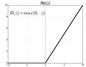
それでは前のモデルにReLUを組み込み、出力を可視化してみましょう。
class Net3(nn.Module):
  """
  Neural Network Instance
  """

  def __init__(self, padding=0):
    """
    Initialize Net3 parameters

    Args:
      padding: int or tuple, optional
        Zero-padding added to both sides of the input. Default: 0

    Returns:
      Nothing
    """
    super(Net3, self).__init__()
    self.conv1 = nn.Conv2d(in_channels=1, out_channels=3, kernel_size=5,
                           padding=padding)

    # First kernel - leading diagonal
    kernel_1 = torch.Tensor([[[1., 1., -1., -1., -1.],
                              [1., 1., 1., -1., -1.],
                              [-1., 1., 1., 1., -1.],
                              [-1., -1., 1., 1., 1.],
                              [-1., -1., -1., 1., 1.]]])

    # Second kernel - other diagonal
    kernel_2 = torch.Tensor([[[-1., -1., -1., 1., 1.],
                              [-1., -1., 1., 1., 1.],
                              [-1., 1., 1., 1., -1.],
                              [1., 1., 1., -1., -1.],
                              [1., 1., -1., -1., -1.]]])

    # Third kernel -checkerboard pattern
    kernel_3 = torch.Tensor([[[1., 1., -1., 1., 1.],
                              [1., 1., 1., 1., 1.],
                              [-1., 1., 1., 1., -1.],
                              [1., 1., 1., 1., 1.],
                              [1., 1., -1., 1., 1.]]])


    # Stack all kernels in one tensor with (3, 1, 5, 5) dimensions
    multiple_kernels = torch.stack([kernel_1, kernel_2, kernel_3], dim=0)

    self.conv1.weight = torch.nn.Parameter(multiple_kernels)

    # Negative bias
    self.conv1.bias = torch.nn.Parameter(torch.Tensor([-4, -4, -12]))

  def forward(self, x):
    """
    Forward Pass of Net3

    Args:
      x: torch.tensor
        Input features

    Returns:
      x: torch.tensor
        Convolution output
    """
    x = self.conv1(x)
    x = F.relu(x)
    return x
フィルターとReLUを画像に適用します。
net3 = Net3().to(DEVICE)
x_img = emnist_train[x_img_idx][0].unsqueeze(dim=0).to(DEVICE)
output_x_relu = net3(x_img)
output_x_relu = output_x_relu.squeeze(dim=0).detach().cpu().numpy()

o_img = emnist_train[o_img_idx][0].unsqueeze(dim=0).to(DEVICE)
output_o_relu = net3(o_img)
output_o_relu = output_o_relu.squeeze(dim=0).detach().cpu().numpy()と の画像と、それらに適用されたフィルターの出力がどのように見えるかを見てみましょう。
# @markdown *Execute this cell to view the filtered images*
fig, ((ax11, ax12, ax13, ax14, ax15, ax16, ax17),
      (ax21, ax22, ax23, ax24, ax25, ax26, ax27),
      (ax31, ax32, ax33, ax34, ax35, ax36, ax37)) = plt.subplots(3, 4 + 3,
                                                                 figsize=(14, 6))
# Show the filters
ax11.axis("off")
ax12.set_title("filter 1")
ax12.imshow(net3.conv1.weight[0, 0].detach().cpu().numpy(), cmap="gray")
ax13.set_title("filter 2")
ax13.imshow(net3.conv1.weight[1, 0].detach().cpu().numpy(), cmap="gray")
ax14.set_title("filter 3")
ax14.imshow(net3.conv1.weight[2, 0].detach().cpu().numpy(), cmap="gray")

ax15.set_title("filter 1")
ax15.imshow(net3.conv1.weight[0, 0].detach().cpu().numpy(), cmap="gray")
ax16.set_title("filter 2")
ax16.imshow(net3.conv1.weight[1, 0].detach().cpu().numpy(), cmap="gray")
ax17.set_title("filter 3")
ax17.imshow(net3.conv1.weight[2, 0].detach().cpu().numpy(), cmap="gray")

vmin, vmax = -6, 10
# Show x and the filters applied to `x`
ax21.set_title("image x")
ax21.imshow(emnist_train[x_img_idx][0].reshape(28, 28), cmap='gray')
ax22.set_title("output filter 1")
ax22.imshow(output_x[0], cmap='gray', vmin=vmin, vmax=vmax)
ax23.set_title("output filter 2")
ax23.imshow(output_x[1], cmap='gray', vmin=vmin, vmax=vmax)
ax24.set_title("output filter 3")
ax24.imshow(output_x[2], cmap='gray', vmin=vmin, vmax=vmax)

ax25.set_title("filter 1 + ReLU")
ax25.imshow(output_x_relu[0], cmap='gray', vmin=vmin, vmax=vmax)
ax26.set_title("filter 2 + ReLU")
ax26.imshow(output_x_relu[1], cmap='gray', vmin=vmin, vmax=vmax)
ax27.set_title("filter 3 + ReLU")
ax27.imshow(output_x_relu[2], cmap='gray', vmin=vmin, vmax=vmax)

# Show o and the filters applied to `o`
ax31.set_title("image o")
ax31.imshow(emnist_train[o_img_idx][0].reshape(28, 28), cmap='gray')
ax32.set_title("output filter 1")
ax32.imshow(output_o[0], cmap='gray', vmin=vmin, vmax=vmax)
ax33.set_title("output filter 2")
ax33.imshow(output_o[1], cmap='gray', vmin=vmin, vmax=vmax)
ax34.set_title("output filter 3")
ax34.imshow(output_o[2], cmap='gray', vmin=vmin, vmax=vmax)

ax35.set_title("filter 1 + ReLU")
ax35.imshow(output_o_relu[0], cmap='gray', vmin=vmin, vmax=vmax)
ax36.set_title("filter 2 + ReLU")
ax36.imshow(output_o_relu[1], cmap='gray', vmin=vmin, vmax=vmax)
ax37.set_title("filter 3 + ReLU")
ax37.imshow(output_o_relu[2], cmap='gray', vmin=vmin, vmax=vmax)
plt.show()
ポッド内で、ReLU 活性化関数が を検出するために必要な特徴をどのように強化するのかについて話し合ってください。
こちらでは、ReLU が活性化関数として有用である理由についての議論が見られます。
こちらでは、ReLU を使う利点についての別の優れた議論が紹介されています。
セクション 3.3: プーリング
畳み込み層は、入力に特定の特徴(例えばエッジ)が存在することを要約した特徴マップを作成します。しかし、これらの特徴マップは入力中の特徴の_正確な_位置を記録しています。つまり、画像内の物体の位置が少し変わるだけで、非常に異なる特徴マップになる可能性があります。しかし、カップはカップであり( は であり)、画像のどこに現れても同じです!私たちは_平行移動不変性_を実現する必要があります。
この問題に対する一般的なアプローチはダウンサンプリングと呼ばれます。ダウンサンプリングは画像の低解像度版を作成し、大きな構造要素を保持しつつ、タスクにあまり関係のない細かいディテールを除去します。CNN では、Max-Pooling と Average-Pooling がダウンサンプリングに使われます。これらの操作は隠れ層のサイズを縮小し、より平行移動不変な特徴を生成し、後続の層でより効果的に利用できます。
# @title Video 4: Pooling
from ipywidgets import widgets
from IPython.display import YouTubeVideo
from IPython.display import IFrame
from IPython.display import display


class PlayVideo(IFrame):
  def __init__(self, id, source, page=1, width=400, height=300, **kwargs):
    self.id = id
    if source == 'Bilibili':
      src = f'https://player.bilibili.com/player.html?bvid={id}&page={page}'
    elif source == 'Osf':
      src = f'https://mfr.ca-1.osf.io/render?url=https://osf.io/download/{id}/?direct%26mode=render'
    super(PlayVideo, self).__init__(src, width, height, **kwargs)


def display_videos(video_ids, W=400, H=300, fs=1):
  tab_contents = []
  for i, video_id in enumerate(video_ids):
    out = widgets.Output()
    with out:
      if video_ids[i][0] == 'Youtube':
        video = YouTubeVideo(id=video_ids[i][1], width=W,
                             height=H, fs=fs, rel=0)
        print(f'Video available at https://youtube.com/watch?v={video.id}')
      else:
        video = PlayVideo(id=video_ids[i][1], source=video_ids[i][0], width=W,
                          height=H, fs=fs, autoplay=False)
        if video_ids[i][0] == 'Bilibili':
          print(f'Video available at https://www.bilibili.com/video/{video.id}')
        elif video_ids[i][0] == 'Osf':
          print(f'Video available at https://osf.io/{video.id}')
      display(video)
    tab_contents.append(out)
  return tab_contents


video_ids = [('Youtube', 'XOss-NUlpo0'), ('Bilibili', 'BV1264y1z7JZ')]
tab_contents = display_videos(video_ids, W=854, H=480)
tabs = widgets.Tab()
tabs.children = tab_contents
for i in range(len(tab_contents)):
  tabs.set_title(i, video_ids[i][0])
display(tabs)
# @title Submit your feedback
content_review(f"{feedback_prefix}_Pooling_Video")畳み込み層と同様に、プーリング層も固定形状のウィンドウ(プーリングウィンドウ)を入力に体系的に適用します。フィルターと同様に、ウィンドウの形状やストライドのサイズを変更できます。そして、フィルターと同じように、プーリング操作を適用するたびに単一の出力を生成します。
プーリングは入力の_近傍_に対する要約統計量を提供する情報圧縮の一種を行います。
- Maxpooling では、プーリングウィンドウ内のすべてのピクセルの最大値を計算します。
- Avgpooling では、プーリングウィンドウ内のすべてのピクセルの平均値を計算します。
以下の例は、黄色のプーリングウィンドウ内で Maxpooling を行い、赤いプーリング出力行列を作成した結果を示しています。

プーリングは各プーリングウィンドウ内の値の要約を提供することでネットワークに平行移動不変性を与えます。したがって、基になる画像の特徴の小さな変化は出力に大きな違いをもたらしません。
畳み込み層とは異なり、プーリング層には学習されるパラメータがありません!プーリングは入力の事前に決められた要約を計算してそれを伝達するだけです。これはフィルターを学習する畳み込み層とは対照的です。
インタラクティブデモ 3.3: ストライドの効果
重要: デモを試すには、ブール変数 run_demo をチェックして True に変更してください。jupyter-book のビデオレンダリングの都合上、自動実行からは外しています。
以下のアニメーションはストライドを変えると出力がどのように変わるかを示しています。ストライドは次の出力を生成するためにプーリング領域が入力行列上でどれだけ移動するかを定義します(アニメーション中の赤い矢印)。ぜひ試してみてください!ストライドを変えて出力の形状がどう変わるか見てみましょう。MaxPool や AvgPool も試せます。
# @markdown *Run this cell to enable the widget!*

from IPython.display import HTML

id_html = 3.3
url = f'https://raw.githubusercontent.com/NeuromatchAcademy/course-content-dl/main/tutorials/W2D2_ConvnetsAndDlThinking/static/interactive_demo{id_html}.html'
run_demo = False # @param {type:"boolean"}
if run_demo:
  display(HTML(url))
# @title Submit your feedback
content_review(f"{feedback_prefix}_The_effect_of_the_stride_Interactive_Demo")コーディング演習 3.3: MaxPooling の実装
それでは PyTorch で MaxPooling を実装し、プーリングが入力画像の次元に与える影響を観察しましょう。MaxPooling 層にはカーネルサイズ 2、ストライド 2 を使ってください。
class Net4(nn.Module):
  """
  Neural Network instance
  """

  def __init__(self, padding=0, stride=2):
    """
    Initialise parameters of Net4

    Args:
      padding: int or tuple, optional
        Zero-padding added to both sides of the input. Default: 0
      stride: int
        Stride

    Returns:
      Nothing
    """
    super(Net4, self).__init__()
    self.conv1 = nn.Conv2d(in_channels=1, out_channels=3, kernel_size=5,
                            padding=padding)

    # First kernel - leading diagonal
    kernel_1 = torch.Tensor([[[1., 1., -1., -1., -1.],
                              [1., 1., 1., -1., -1.],
                              [-1., 1., 1., 1., -1.],
                              [-1., -1., 1., 1., 1.],
                              [-1., -1., -1., 1., 1.]]])

    # Second kernel - other diagonal
    kernel_2 = torch.Tensor([[[-1., -1., -1., 1., 1.],
                              [-1., -1., 1., 1., 1.],
                              [-1., 1., 1., 1., -1.],
                              [1., 1., 1., -1., -1.],
                              [1., 1., -1., -1., -1.]]])

    # Third kernel -checkerboard pattern
    kernel_3 = torch.Tensor([[[1., 1., -1., 1., 1.],
                              [1., 1., 1., 1., 1.],
                              [-1., 1., 1., 1., -1.],
                              [1., 1., 1., 1., 1.],
                              [1., 1., -1., 1., 1.]]])


    # Stack all kernels in one tensor with (3, 1, 5, 5) dimensions
    multiple_kernels = torch.stack([kernel_1, kernel_2, kernel_3], dim=0)

    self.conv1.weight = torch.nn.Parameter(multiple_kernels)

    # Negative bias
    self.conv1.bias = torch.nn.Parameter(torch.Tensor([-4, -4, -12]))
    ####################################################################
    # Fill in missing code below (...),
    # then remove or comment the line below to test your function
    raise NotImplementedError("Define the maxpool layer")
    ####################################################################
    self.pool = nn.MaxPool2d(kernel_size=..., stride=...)

  def forward(self, x):
    """
    Forward Pass of Net4

    Args:
      x: torch.tensor
        Input features

    Returns:
      x: torch.tensor
        Convolution + ReLU output
    """
    x = self.conv1(x)
    x = F.relu(x)
    ####################################################################
    # Fill in missing code below (...),
    # then remove or comment the line below to test your function
    raise NotImplementedError("Define the maxpool layer")
    ####################################################################
    x = ...  # Pass through a max pool layer
    return x


## Check if your implementation is correct
# net4 = Net4().to(DEVICE)
# check_pooling_net(net4, device=DEVICE)
✅ ネットワークは正しい出力を生成しました。
# @title Submit your feedback
content_review(f"{feedback_prefix}_Implement_MaxPooling_Exercise")
x_img = emnist_train[x_img_idx][0].unsqueeze(dim=0).to(DEVICE)
output_x_pool = net4(x_img)
output_x_pool = output_x_pool.squeeze(dim=0).detach().cpu().numpy()
o_img = emnist_train[o_img_idx][0].unsqueeze(dim=0).to(DEVICE)
output_o_pool = net4(o_img)
output_o_pool = output_o_pool.squeeze(dim=0).detach().cpu().numpy()# @markdown *Run the cell to plot the outputs!*
fig, ((ax11, ax12, ax13, ax14),
(ax21, ax22, ax23, ax24),
(ax31, ax32, ax33, ax34)) = plt.subplots(3, 4)
# Show the filters
ax11.axis("off")
ax12.set_title("filter 1")
ax12.imshow(net4.conv1.weight[0, 0].detach().cpu().numpy(), cmap="gray")
ax13.set_title("filter 2")
ax13.imshow(net4.conv1.weight[1, 0].detach().cpu().numpy(), cmap="gray")
ax14.set_title("filter 3")
ax14.imshow(net4.conv1.weight[2, 0].detach().cpu().numpy(), cmap="gray")
vmin, vmax = -6, 10
# Show x and the filters applied to x
ax21.set_title("image x")
ax21.imshow(emnist_train[x_img_idx][0].reshape(28, 28), cmap='gray')
ax22.set_title("output filter 1")
ax22.imshow(output_x_pool[0], cmap='gray', vmin=vmin, vmax=vmax)
ax23.set_title("output filter 2")
ax23.imshow(output_x_pool[1], cmap='gray', vmin=vmin, vmax=vmax)
ax24.set_title("output filter 3")
ax24.imshow(output_x_pool[2], cmap='gray', vmin=vmin, vmax=vmax)
# Show o and the filters applied to o
ax31.set_title("image o")
ax31.imshow(emnist_train[o_img_idx][0].reshape(28, 28), cmap='gray')
ax32.set_title("output filter 1")
ax32.imshow(output_o_pool[0], cmap='gray', vmin=vmin, vmax=vmax)
ax33.set_title("output filter 2")
ax33.imshow(output_o_pool[1], cmap='gray', vmin=vmin, vmax=vmax)
ax34.set_title("output filter 3")
ax34.imshow(output_o_pool[2], cmap='gray', vmin=vmin, vmax=vmax)
plt.show()ReLU セクションの後に見た出力のサイズの半分になっていることが観察できるはずです。これは Maxpool 層によるものです。
出力のサイズは減少しましたが、出力内の重要な高レベルの特徴は依然として保持されています。
セクション 4: まとめ
所要時間の目安: 約33分
# @title Video 5: Putting it all together
from ipywidgets import widgets
from IPython.display import YouTubeVideo
from IPython.display import IFrame
from IPython.display import display


class PlayVideo(IFrame):
  def __init__(self, id, source, page=1, width=400, height=300, **kwargs):
    self.id = id
    if source == 'Bilibili':
      src = f'https://player.bilibili.com/player.html?bvid={id}&page={page}'
    elif source == 'Osf':
      src = f'https://mfr.ca-1.osf.io/render?url=https://osf.io/download/{id}/?direct%26mode=render'
    super(PlayVideo, self).__init__(src, width, height, **kwargs)


def display_videos(video_ids, W=400, H=300, fs=1):
  tab_contents = []
  for i, video_id in enumerate(video_ids):
    out = widgets.Output()
    with out:
      if video_ids[i][0] == 'Youtube':
        video = YouTubeVideo(id=video_ids[i][1], width=W,
                             height=H, fs=fs, rel=0)
        print(f'Video available at https://youtube.com/watch?v={video.id}')
      else:
        video = PlayVideo(id=video_ids[i][1], source=video_ids[i][0], width=W,
                          height=H, fs=fs, autoplay=False)
        if video_ids[i][0] == 'Bilibili':
          print(f'Video available at https://www.bilibili.com/video/{video.id}')
        elif video_ids[i][0] == 'Osf':
          print(f'Video available at https://osf.io/{video.id}')
      display(video)
    tab_contents.append(out)
  return tab_contents


video_ids = [('Youtube', '-TJixd9fRCw'), ('Bilibili', 'BV1Fy4y1j7dU')]
tab_contents = display_videos(video_ids, W=854, H=480)
tabs = widgets.Tab()
tabs.children = tab_contents
for i in range(len(tab_contents)):
  tabs.set_title(i, video_ids[i][0])
display(tabs)
# @title Submit your feedback
content_review(f"{feedback_prefix}_Putting_it_all_together_Video")セクション 4.1: 畳み込みモデルと全結合モデルのパラメータ数
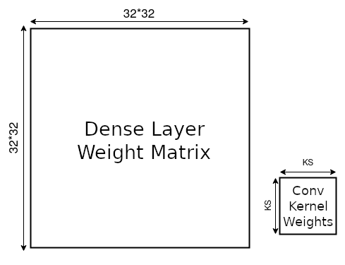
畳み込みネットワークは、入力画像全体に繰り返し適用される単一のカーネルを学習することで重みの共有を促進します。一般に、このカーネルは数個のパラメータしか持たず、全結合ネットワークの膨大なパラメータ数と比べて非常に少ないです。
以下のアニメーションを使って、 の画像データに対して畳み込み層と全結合層の両方を用いた数層のネットワークのパラメータ数を計算してみましょう。この演習の Num_Dense はネットワークで使う全結合層の数で、各全結合層は同じ入力・出力次元を持ちます。Num_Convs はネットワーク内の畳み込みブロックの数で、各ブロックは単一のカーネルを含みます。カーネルサイズはこのカーネルの縦横の長さです。
注意: スライダーを使う前にセルを実行する必要があります。
インタラクティブデモ 4.1: パラメータ数
# @markdown *Run this cell to enable the widget*
import io, base64
from ipywidgets import interact, interactive, fixed, interact_manual


def do_plot(image_size, batch_size, number_of_Linear, number_of_Conv2d,
            kernel_size, pooling, Final_Layer):
  sample_image = torch.rand(batch_size, 1, image_size, image_size)
  linear_layer = []
  linear_nets = []
  code_dense = ""

  code_dense += f"model_dense = nn.Sequential(\n"
  code_dense += f"    nn.Flatten(),\n"
  for i in range(number_of_Linear):
    linear_layer.append(nn.Linear(image_size * image_size * 1,
                                  image_size * image_size * 1,
                                  bias=False))
    linear_nets.append(nn.Sequential(*linear_layer))
    code_dense += f"    nn.Linear({image_size}*{image_size}*1, {image_size}*{image_size}*1, bias=False),\n"
  if Final_Layer is True:
    linear_layer.append(nn.Linear(image_size * image_size * 1, 10,
                                  bias=False))
    linear_nets.append(nn.Sequential(*linear_layer))
    code_dense += f"    nn.Linear({image_size}*{image_size}*1, 10, bias=False)\n"
  code_dense += ")\n"
  code_dense += "result_dense = model_dense(sample_image)\n"
  linear_layer = nn.Sequential(*linear_layer)

  conv_layer = []
  conv_nets = []
  code_conv = ""

  code_conv += f"model_conv = nn.Sequential(\n"
  for i in range(number_of_Conv2d):
    conv_layer.append(nn.Conv2d(in_channels=1,
                                out_channels=1,
                                kernel_size=kernel_size,
                                padding=kernel_size // 2,
                                bias=False))

    conv_nets.append(nn.Sequential(*conv_layer))
    code_conv += f"    nn.Conv2d(in_channels=1, out_channels=1, kernel_size={kernel_size}, padding={kernel_size//2}, bias=False),\n"
    if pooling > 0:
      conv_layer.append(nn.MaxPool2d(2, 2))
      code_conv += f"    nn.MaxPool2d(2, 2),\n"
    conv_nets.append(nn.Sequential(*conv_layer))
  if Final_Layer is True:
    conv_layer.append(nn.Flatten())
    code_conv += f"    nn.Flatten(),\n"
    conv_nets.append(nn.Sequential(*conv_layer))
    shape_conv = conv_nets[-1](sample_image).shape
    conv_layer.append(nn.Linear(shape_conv[1], 10, bias=False))
    code_conv += f"    nn.Linear({shape_conv[1]}, 10, bias=False),\n"
    conv_nets.append(nn.Sequential(*conv_layer))
  conv_layer = nn.Sequential(*conv_layer)
  code_conv += ")\n"
  code_conv += "result_conv = model_conv(sample_image)\n"


  t_1 = time.time()
  shape_linear = linear_layer(torch.flatten(sample_image, 1)).shape
  t_2 = time.time()
  shape_conv = conv_layer(sample_image).shape
  t_3 = time.time()

  print("Time taken by Dense Layer {}".format(t_2 - t_1))
  print("Time taken by Conv Layer  {}".format(t_3 - t_2))

  ax = plt.axes((0, 0, 1, 1))
  ax.spines["left"].set_visible(False)
  plt.yticks([])
  ax.spines["bottom"].set_visible(False)
  ax.spines["right"].set_visible(False)
  ax.spines["top"].set_visible(False)
  plt.xticks([])
  p1 = sum(p.numel() for p in linear_layer.parameters())
  nl = '\n'
  p2 = sum(p.numel() for p in conv_layer.parameters())
  plt.text(0.1, 0.8,
           f"Total Parameters in Dense Layer {p1:10,d}{nl}Total Parameters in Conv Layer   {p2:10,d}")

  plt.text(0.23, 0.62, "Dense Net", rotation=90,
           color='k', ha="center", va="center")

  def addBox(x, y, w, h, color, text1, text2, text3):
      """
      Function to render widget
      """
      ax.add_patch(plt.Rectangle((x, y), w, h, fill=True, color=color,
                                 alpha=0.5, zorder=1000, clip_on=False))
      plt.text(x + 0.02, y + h / 2, text1, rotation=90,
               va="center", ha="center", size=12)
      plt.text(x + 0.05, y + h / 2, text2, rotation=90,
               va="center", ha="center")
      plt.text(x + 0.08, y + h / 2, text3, rotation=90,
               va="center", ha="center", size=12)

  x = 0.25
  if 1:
    addBox(x, 0.5, 0.08, 0.25, [1, 0.5, 0], "Flatten",
           tuple(torch.flatten(sample_image, 1).shape), "")
    x += 0.08 + 0.01

  for i in range(number_of_Linear):
    addBox(x, 0.5, 0.1, 0.25, "g", "Dense",
           tuple(linear_nets[i](torch.flatten(sample_image, 1)).shape),
           list(linear_layer.parameters())[i].numel())
    x += 0.11

  if Final_Layer is True:
    i = number_of_Linear
    addBox(x, 0.5, 0.1, 0.25, "g", "Dense",
           tuple(linear_nets[i](torch.flatten(sample_image, 1)).shape),
           list(linear_layer.parameters())[i].numel())

  plt.text(0.23, 0.1 + 0.35 / 2, "Conv Net",
           rotation=90, color='k',
           ha="center", va="center")
  x = 0.25

  for i in range(number_of_Conv2d):
    addBox(x, 0.1, 0.1, 0.35, "r", "Conv",
           tuple(conv_nets[i * 2](sample_image).shape),
           list(conv_nets[i * 2].parameters())[-1].numel())
    x += 0.11
    if pooling > 0:
      addBox(x, 0.1, 0.08, 0.35, [0, 0.5, 1], "Pooling",
             tuple(conv_nets[i * 2 + 1](sample_image).shape), "")
      x += 0.08 + 0.01

  if Final_Layer is True:
    i = number_of_Conv2d
    addBox(x, 0.1, 0.08, 0.35, [1, 0.5, 0], "Flatten",
           tuple(conv_nets[i * 2](sample_image).shape), "")
    x += 0.08 + 0.01

    addBox(x, 0.1, 0.1, 0.35, "g", "Dense",
            tuple(conv_nets[i * 2 + 1](sample_image).shape),
            list(conv_nets[i * 2 + 1].parameters())[-1].numel())
    x += 0.11

  plt.text(0.08, 0.3 + 0.35 / 2,
           "Input", rotation=90, color='b', ha="center", va="center")

  ax.add_patch(plt.Rectangle((0.1, 0.3), 0.1, 0.35, fill=True, color='b',
                             alpha=0.5, zorder=1000, clip_on=False))
  plt.text(0.1 + 0.1 / 2, 0.3 + 0.35 / 2, tuple(sample_image.shape),
           rotation=90, va="center", ha="center")

  # Plot
  plt.gcf().set_tight_layout(False)
  my_stringIObytes = io.BytesIO()
  plt.savefig(my_stringIObytes, format='png', dpi=90)
  my_stringIObytes.seek(0)
  my_base64_jpgData = base64.b64encode(my_stringIObytes.read())

  del linear_layer, conv_layer

  plt.close()
  mystring = """<img src="data:image/png;base64,""" + str(my_base64_jpgData)[2:-1] + """" alt="Graph">"""

  return code_dense, code_conv, mystring


# Parameters
caption = widgets.Label(value='The values of range1 and range2 are synchronized')
slider_batch_size = widgets.IntSlider(value=100, min=10, max=100, step=10,
                                      description="BatchSize")
slider_image_size = widgets.IntSlider(value=32, min=32, max=128, step=32,
                                      description="ImageSize")
slider_number_of_Linear = widgets.IntSlider(value=1,min=1, max=3, step=1,
                                            description="NumDense")
slider_number_of_Conv2d = widgets.IntSlider(value=1, min=1, max=2, step=1,
                                            description="NumConv")
slider_kernel_size = widgets.IntSlider(value=5, min=3, max=21, step=2,
                                       description="KernelSize")
input_pooling = widgets.Checkbox(value=False,
                                 description="Pooling")
input_Final_Layer = widgets.Checkbox(value=False,
                                     description="Final_Layer")

output_code1 = widgets.HTML(value="", )

output_plot = widgets.HTML(value="", )


def plot_func(batch_size, image_size,
              number_of_Linear, number_of_Conv2d,
              kernel_size, pooling, Final_Layer):

    code1, code2, plot = do_plot(image_size, batch_size,
                                 number_of_Linear, number_of_Conv2d,
                                 kernel_size, pooling, Final_Layer)
    output_plot.value = plot

    output_code1.value = """
    <!DOCTYPE html>
    <html>
      <head>
        <style>
          * {
            box-sizing: border-box;
          }
          .column {
            float: left;
            /*width: 33.33%;*/
            padding: 5px;
          }
          /* Clearfix (clear floats) */
          .row::after {
            content: "";
            clear: both;
            display: table;
          }
          pre {
            line-height: 1.2em;
          }
        </style>
      </head>

      <body>
        <div class="row">
          <div class="column" style="overflow-x: scroll;">
          <h2>Code for Dense Network</h2>
          <pre>""" + code1 + """</pre>
        </div>
          <div class="column" style="overflow-x: scroll;">
          <h2>Code for Conv Network</h2>
          <pre>""" + code2 + """</pre>
          </div>
        </div>
      </body>
    </html>
"""

out = widgets.interactive_output(plot_func, {
    "batch_size": slider_batch_size,
    "image_size": slider_image_size,
    "number_of_Linear": slider_number_of_Linear,
    "number_of_Conv2d": slider_number_of_Conv2d,
    "kernel_size": slider_kernel_size,
    "pooling": input_pooling,
    "Final_Layer": input_Final_Layer,
})

ui = widgets.VBox([slider_batch_size, slider_image_size,
                   slider_number_of_Linear,
                   widgets.HBox([slider_number_of_Conv2d,
                                 slider_kernel_size,
                                 input_pooling]),
                   input_Final_Layer])
display(widgets.HBox([output_plot, output_code1]), ui)
display(out)
パラメータの差は非常に大きく、入力画像サイズが大きくなるにつれてさらに増加します。大きな画像では、線形層が入力ピクセルと直接掛け算できる行列を使用する必要があります。
プーリングは後続の畳み込み層のパラメータ数を減らしませんが、画像サイズを小さくします。したがって、後の全結合層はより少ないパラメータで済みます。
しかし、CNNのパラメータサイズは画像サイズに依存しません。入力に関わらず、同じ学習可能なフィルターを画像上でスライドさせ続けるためです。
パラメータ数の削減は、メモリ使用量を大幅に減らすだけでなく、モデルの汎化性能向上にも寄与します。
# @title Submit your feedback
content_review(f"{feedback_prefix}_Number_of_Parameters_Interactive_Demo")
# @title Video 6: Implement your own CNN
from ipywidgets import widgets
from IPython.display import YouTubeVideo
from IPython.display import IFrame
from IPython.display import display
class PlayVideo(IFrame):
def __init__(self, id, source, page=1, width=400, height=300, **kwargs):
self.id = id
if source == 'Bilibili':
src = f'https://player.bilibili.com/player.html?bvid={id}&page={page}'
elif source == 'Osf':
src = f'https://mfr.ca-1.osf.io/render?url=https://osf.io/download/{id}/?direct%26mode=render'
super(PlayVideo, self).__init__(src, width, height, **kwargs)
def display_videos(video_ids, W=400, H=300, fs=1):
tab_contents = []
for i, video_id in enumerate(video_ids):
out = widgets.Output()
with out:
if video_ids[i][0] == 'Youtube':
video = YouTubeVideo(id=video_ids[i][1], width=W,
height=H, fs=fs, rel=0)
print(f'Video available at https://youtube.com/watch?v={video.id}')
else:
video = PlayVideo(id=video_ids[i][1], source=video_ids[i][0], width=W,
height=H, fs=fs, autoplay=False)
if video_ids[i][0] == 'Bilibili':
print(f'Video available at https://www.bilibili.com/video/{video.id}')
elif video_ids[i][0] == 'Osf':
print(f'Video available at https://osf.io/{video.id}')
display(video)
tab_contents.append(out)
return tab_contents
video_ids = [('Youtube', '_gkF9Vv7MgE'), ('Bilibili', 'BV18f4y1j7e4')]
tab_contents = display_videos(video_ids, W=854, H=480)
tabs = widgets.Tab()
tabs.children = tab_contents
for i in range(len(tab_contents)):
tabs.set_title(i, video_ids[i][0])
display(tabs)# @title Submit your feedback
content_review(f"{feedback_prefix}_Implement_your_own_CNN_Video")コーディング演習4: 自分のCNNを実装しよう
これまで学んだことをすべて積み重ねましょう。以下の構造のCNNを作成してください。
- 畳み込み層
nn.Conv2d(in_channels=1, out_channels=32, kernel_size=3) - 畳み込み層
nn.Conv2d(in_channels=32, out_channels=64, kernel_size=3) - プーリング層
- 全結合層
nn.Linear(in_features=9216, out_features=128) - 全結合層
nn.Linear(in_features=128, out_features=2)
注意:動画で説明したように、線形層に渡す前に畳み込み層の出力をフラット化(flatten)します。つまり、入力の形状 を に変換します。今回の場合、2番目の畳み込み層の出力 を に変換します。入力画像のサイズは です。
ヒント:この段階で入力をフラット化するには torch.flatten(x, 1) を使うと良いです。ここでの はバッチ次元を除いて次元1以降をフラット化することを意味します。
また、プーリング層の出力が になる理由についても考えましょう。最初の2つの Conv2d(カーネルサイズ3)が画像サイズをそれぞれ 、 に減少させ、最後に MaxPool2d によって出力サイズが半分の になります。
さらに、ReLUも忘れずに(例:F.relu を使用)!最終の全結合層の後にはReLUは不要です。
# @title Train/Test Functions (Run Me)

# @markdown Double-click to see the contents!

def train(model, device, train_loader, epochs):
  """
  Training function

  Args:
    model: nn.module
      Neural network instance
    device: string
      GPU/CUDA if available, CPU otherwise
    epochs: int
      Number of epochs
    train_loader: torch.loader
      Training Set

  Returns:
    Nothing
  """
  model.train()

  criterion = nn.CrossEntropyLoss()
  optimizer = torch.optim.SGD(model.parameters(), lr=0.01)
  for epoch in range(epochs):
    with tqdm(train_loader, unit='batch') as tepoch:
      for data, target in tepoch:
        data, target = data.to(device), target.to(device)
        optimizer.zero_grad()
        output = model(data)

        loss = criterion(output, target)
        loss.backward()
        optimizer.step()
        tepoch.set_postfix(loss=loss.item())
        time.sleep(0.1)

def test(model, device, data_loader):
  """
  Test function

  Args:
    model: nn.module
      Neural network instance
    device: string
      GPU/CUDA if available, CPU otherwise
    data_loader: torch.loader
      Test Set

  Returns:
    acc: float
      Test accuracy
  """
  model.eval()
  correct = 0
  total = 0
  for data in data_loader:
    inputs, labels = data
    inputs = inputs.to(device).float()
    labels = labels.to(device).long()

    outputs = model(inputs)
    _, predicted = torch.max(outputs, 1)
    total += labels.size(0)
    correct += (predicted == labels).sum().item()

  acc = 100 * correct / total
  return acc
データをダウンロードします。ここではデータセットを正規化していることに注意してください。
set_seed(SEED)
emnist_train, emnist_test = get_Xvs0_dataset(normalize=True)
train_loader, test_loader = get_data_loaders(emnist_train, emnist_test,
                                             seed=SEED)
class EMNIST_Net(nn.Module):
"""
Neural network instance with following structure
nn.Conv2d(in_channels=1, out_channels=32, kernel_size=3) # Convolutional Layer 1
nn.Conv2d(in_channels=32, out_channels=64, kernel_size=3) + max-pooling # Convolutional Block 2
nn.Linear(in_features=9216, out_features=128) # Fully Connected Layer 1
nn.Linear(in_features=128, out_features=2) # Fully Connected Layer 2
"""
def __init__(self):
"""
Initialize parameters of EMNISTNet
Args:
None
Returns:
Nothing
"""
super(EMNIST_Net, self).__init__()
####################################################################
# Fill in missing code below (...),
# then remove or comment the line below to test your function
raise NotImplementedError("Define the required layers")
####################################################################
self.conv1 = nn.Conv2d(...)
self.conv2 = nn.Conv2d(...)
self.fc1 = nn.Linear(...)
self.fc2 = nn.Linear(...)
self.pool = nn.MaxPool2d(...)
def forward(self, x):
"""
Forward pass of EMNISTNet
Args:
x: torch.tensor
Input features
Returns:
x: torch.tensor
Output of final fully connected layer
"""
####################################################################
# Fill in missing code below (...),
# then remove or comment the line below to test your function
# Hint: Do not forget to flatten the image as it goes from
# Convolution Layers to Linear Layers!
raise NotImplementedError("Define forward pass for any input x")
####################################################################
x = self.conv1(x)
x = F.relu(x)
x = self.conv2(x)
x = ...
x = ...
x = ...
x = ...
x = ...
x = ...
return x
## Uncomment the lines below to train your network
# emnist_net = EMNIST_Net().to(DEVICE)
# print("Total Parameters in Network {:10d}".format(sum(p.numel() for p in emnist_net.parameters())))
# train(emnist_net, DEVICE, train_loader, 1)
## Uncomment to test your model
# print(f'Test accuracy is: {test(emnist_net, DEVICE, test_loader)}')テスト精度は約 を達成できたはずです!
# @title Submit your feedback
content_review(f"{feedback_prefix}_Implement_your_own_CNN_Exercise")
注意: ここではソフトマックス関数を使用しており、実数値を0から1の範囲に変換し、確率として解釈できるようにしています。
# Index of an image in the dataset that corresponds to an X and O
x_img_idx = 11
o_img_idx = 0

print("Input:")
x_img = emnist_train[x_img_idx][0].unsqueeze(dim=0).to(DEVICE)
plt.imshow(emnist_train[x_img_idx][0].reshape(28, 28),
           cmap=plt.get_cmap('gray'))
plt.show()
output = emnist_net(x_img)
result = F.softmax(output, dim=1)
print("\nResult:", result)
print("Confidence of image being an 'O':", result[0, 0].item())
print("Confidence of image being an 'X':", result[0, 1].item())
ネットワークはこの画像が であるとかなり自信を持っています!
これはソフトマックスの出力からも明らかで、各クラスに属する確率を示しています。クラス1、つまりクラス に属する確率が高いです。
次に、 の画像でネットワークをテストしてみましょう。
print("Input:")
o_img = emnist_train[o_img_idx][0].unsqueeze(dim=0).to(DEVICE)
plt.imshow(emnist_train[o_img_idx][0].reshape(28, 28),
           cmap=plt.get_cmap('gray'))
plt.show()
output = emnist_net(o_img)
result = F.softmax(output, dim=1)
print("\nResult:", result)
print("Confidence of image being an 'O':", result[0, 0].item())
print("Confidence of image being an 'X':", result[0, 1].item())
まとめ
このチュートリアルではCNNに慣れ親しみました。畳み込み演算の仕組みと画像への適用方法を学びました。また、自分でCNNを実装する方法も習得しました。次のチュートリアルではCNNのトレーニングについてさらに深く学びます!
ボーナス1: 自分のトレーニングループを再考する
所要時間の目安:約20分
前のセクションではCNNをコーディングしましたが、あらかじめ用意された関数でトレーニングしました。このセクションでは、畳み込みネットワークのトレーニングループの例を順を追って説明します。畳み込み層とマックスプーリングを使ってCNNをトレーニングし、トレーニング曲線と検証曲線を観察します。セクション6では正則化とデータ拡張を追加し、それらが曲線に与える影響とトレーニング時に取り入れる重要性を見ていきます。
# @title Video 7: Writing your own training loop
from ipywidgets import widgets
from IPython.display import YouTubeVideo
from IPython.display import IFrame
from IPython.display import display


class PlayVideo(IFrame):
  def __init__(self, id, source, page=1, width=400, height=300, **kwargs):
    self.id = id
    if source == 'Bilibili':
      src = f'https://player.bilibili.com/player.html?bvid={id}&page={page}'
    elif source == 'Osf':
      src = f'https://mfr.ca-1.osf.io/render?url=https://osf.io/download/{id}/?direct%26mode=render'
    super(PlayVideo, self).__init__(src, width, height, **kwargs)


def display_videos(video_ids, W=400, H=300, fs=1):
  tab_contents = []
  for i, video_id in enumerate(video_ids):
    out = widgets.Output()
    with out:
      if video_ids[i][0] == 'Youtube':
        video = YouTubeVideo(id=video_ids[i][1], width=W,
                             height=H, fs=fs, rel=0)
        print(f'Video available at https://youtube.com/watch?v={video.id}')
      else:
        video = PlayVideo(id=video_ids[i][1], source=video_ids[i][0], width=W,
                          height=H, fs=fs, autoplay=False)
        if video_ids[i][0] == 'Bilibili':
          print(f'Video available at https://www.bilibili.com/video/{video.id}')
        elif video_ids[i][0] == 'Osf':
          print(f'Video available at https://osf.io/{video.id}')
      display(video)
    tab_contents.append(out)
  return tab_contents


video_ids = [('Youtube', 'L0XG-QKv5_w'), ('Bilibili', 'BV1Ko4y1Q7UG')]
tab_contents = display_videos(video_ids, W=854, H=480)
tabs = widgets.Tab()
tabs.children = tab_contents
for i in range(len(tab_contents)):
  tabs.set_title(i, video_ids[i][0])
display(tabs)
# @title Submit your feedback
content_review(f"{feedback_prefix}_Writing_your_own_training_loop_Bonus_Video")ボーナス1.1: データセットを理解しよう
この課題で使用するデータセットはFashion-MNISTです。トレーニングセットは60,000例、テストセットは10,000例あります。テストセットはさらに検証セット(8,000例)とテストセット(2,000例)に分割します。各例は のグレースケール画像で、10クラスのラベルが付いています。データセットのラベルは以下の通りです:
\begin{matrix}
&& \
\hline
0 && \
1 && \
2 && \
3 && \
4 && \
5 && \
6 && \
7 && \
8 && \
9 && \
\end{matrix}
注意: トレーニング時間を約10分から2分に短縮するため、データセットをTシャツ/トップとシャツの2カテゴリのみに絞ります。後で全データセットでの結果例も提供し、全体の結果イメージを掴めるようにします。
# @title Download Fashion MNIST dataset

# webpage: https://github.com/zalandoresearch/fashion-mnist
fname = 'FashionMNIST.tar.gz'
folder = 'FashionMNIST'
url = "https://osf.io/dfhu5/download"
download_data(fname, folder, url, tar=True)
# @title Loading Fashion-MNIST Data
# @markdown `reduce_classes(data)` to reduce Fashion-MNIST Data to two-categories
# need to split into train, validation, test
def reduce_classes(data):
"""
Reducing classes in Fashion MNIST
to T-Shirts and Shirts
Args:
data: torch.tensor
Training Data
Returns:
data: torch.tensor
Data with two classes
"""
# Only want T-Shirts (0) and Shirts (6) labels
train_idx = (data.targets == 0) | (data.targets == 6)
data.targets = data.targets[train_idx]
data.data = data.data[train_idx]
# Convert Xs predictions to 1, Os predictions to 0
data.targets[data.targets == 6] = 1
return data
def get_fashion_mnist_dataset(binary=False, download=False, seed=0):
"""
Helper function to get Fashion MNIST data
Args:
binary: boolean
If True, training data has only two classes
download: boolean
If True, download training data
seed: int
Set seed for reproducibility [default: 0]
Returns:
train_data: torch.tensor
Training data
test_data: torch.tensor
Test data
validation_data: torch.tensor
Validation data
"""
transform = transforms.Compose([
transforms.ToTensor(),
transforms.Normalize((0.1307,), (0.3081,))
])
train_data = datasets.FashionMNIST(root='.',
download=download,
train=True,
transform=transform)
test_data = datasets.FashionMNIST(root='.',
download=download,
train=False,
transform=transform)
if binary:
train_data = reduce_classes(train_data)
test_data = reduce_classes(test_data)
set_seed(seed)
validation_data, test_data = torch.utils.data.random_split(test_data,
[int(0.8*len(test_data)),
int(0.2*len(test_data))])
return train_data, validation_data, test_datanum_classes = 10
train_data, validation_data, test_data = get_fashion_mnist_dataset(seed=SEED)10クラスのデータセットで続けたい場合は、次のセルをスキップしてください。
num_classes = 2
train_data, validation_data, test_data = get_fashion_mnist_dataset(binary=True, seed=SEED)
データセットを可視化するためのコードです。
fig, (ax1, ax2, ax3, ax4) = plt.subplots(1, 4)
ax1.imshow(train_data[0][0].reshape(28, 28), cmap=plt.get_cmap('gray'))
ax2.imshow(train_data[1][0].reshape(28, 28), cmap=plt.get_cmap('gray'))
ax3.imshow(train_data[2][0].reshape(28, 28), cmap=plt.get_cmap('gray'))
ax4.imshow(train_data[3][0].reshape(28, 28), cmap=plt.get_cmap('gray'))
fig.set_size_inches(18.5, 10.5)
plt.show()
ポッドのメンバーと少し話し合って、どのクラスが最も混同しやすいと思うか考えてみましょう。Tシャツ/トップスとシャツを区別するのはどれくらい難しいでしょうか?
# @title Video 8: The Training Loop
from ipywidgets import widgets
from IPython.display import YouTubeVideo
from IPython.display import IFrame
from IPython.display import display


class PlayVideo(IFrame):
  def __init__(self, id, source, page=1, width=400, height=300, **kwargs):
    self.id = id
    if source == 'Bilibili':
      src = f'https://player.bilibili.com/player.html?bvid={id}&page={page}'
    elif source == 'Osf':
      src = f'https://mfr.ca-1.osf.io/render?url=https://osf.io/download/{id}/?direct%26mode=render'
    super(PlayVideo, self).__init__(src, width, height, **kwargs)


def display_videos(video_ids, W=400, H=300, fs=1):
  tab_contents = []
  for i, video_id in enumerate(video_ids):
    out = widgets.Output()
    with out:
      if video_ids[i][0] == 'Youtube':
        video = YouTubeVideo(id=video_ids[i][1], width=W,
                             height=H, fs=fs, rel=0)
        print(f'Video available at https://youtube.com/watch?v={video.id}')
      else:
        video = PlayVideo(id=video_ids[i][1], source=video_ids[i][0], width=W,
                          height=H, fs=fs, autoplay=False)
        if video_ids[i][0] == 'Bilibili':
          print(f'Video available at https://www.bilibili.com/video/{video.id}')
        elif video_ids[i][0] == 'Osf':
          print(f'Video available at https://osf.io/{video.id}')
      display(video)
    tab_contents.append(out)
  return tab_contents


video_ids = [('Youtube', 'ZgYYgktqaP8'), ('Bilibili', 'BV1av411n7VJ')]
tab_contents = display_videos(video_ids, W=854, H=480)
tabs = widgets.Tab()
tabs.children = tab_contents
for i in range(len(tab_contents)):
  tabs.set_title(i, video_ids[i][0])
display(tabs)
# @title Submit your feedback
content_review(f"{feedback_prefix}_The_training_loop_Bonus_Video")ボーナス 1.2: 逆伝播の復習
逆伝播がしっかり理解できている場合はスキップしても構いません
入力データやテンソルに重み行列を掛けて出力を得ることは知っています。最初は実際の重み行列がわからないため、ランダムな値で初期化します。これらのランダムな重み行列を入力に適用すると、ある出力が得られます。最初は出力や予測が正しいラベルと一致するのは偶然に過ぎません。
性能を向上させるために、予測出力が真の出力(ラベル)に近くなるように重み行列を変更する必要があります。まず損失関数を使って予測出力と真の出力の差を計算します。損失関数に基づいて、誤差の重み行列に対する勾配を用いて重み行列の値を変更します。
このコースではPyTorchを使用しているため、組み込み関数で重みを更新します。'loss'変数に対してbackward()メソッドを呼び出し、すべての重み行列とバイアスに関する勾配・微分を計算します。その後、optimizer変数のstep()メソッドを呼び出して勾配更新を重み行列に適用します。
逆伝播の動作を示すアニメーションです。
こちらの記事ではさらに多くのアニメーションを見ることができます!
まずはサンプルトレーニングループを見てみましょう。最初にネットワークを作成し、データセットを読み込みます。次にトレーニングループを見ていきます。
class emnist_net(nn.Module):
  """
  Create a sample network
  """

  def __init__(self):
    """
    Initialise parameters of sample network

    Args:
      None

    Returns:
      Nothing
    """
    super().__init__()
    # First define the layers.
    self.conv1 = nn.Conv2d(1, 32, kernel_size=5, padding=2)
    self.conv2 = nn.Conv2d(32, 64, kernel_size=5, padding=2)
    self.fc1 = nn.Linear(7 * 7 * 64, 256)
    self.fc2 = nn.Linear(256, 26)

  def forward(self, x):
    """
    Forward pass of sample network

    Args:
      x: torch.tensor
        Input features

    Returns:
      x: torch.tensor
        Output after passing through sample network
    """
    # Conv layer 1.
    x = self.conv1(x)
    x = F.relu(x)
    x = F.max_pool2d(x, kernel_size=2)

    # Conv layer 2.
    x = self.conv2(x)
    x = F.relu(x)
    x = F.max_pool2d(x, kernel_size=2)

    # Fully connected layer 1.
    x = x.view(-1, 7 * 7 * 64)  # You have to first flatten the ourput from the
                            # previous convolution layer.
    x = self.fc1(x)
    x = F.relu(x)

    # Fully connected layer 2.
    x = self.fc2(x)

    return x
# @title Load a sample dataset (EMNIST)
# Download the data if there are not downloaded
fname = 'EMNIST.zip'
folder = 'EMNIST'
url = "https://osf.io/xwfaj/download"
download_data(fname, folder, url, tar=False)
mnist_train = datasets.EMNIST(root=".",
train=True,
transform=transforms.ToTensor(),
download=False,
split='letters')
mnist_test = datasets.EMNIST(root=".",
train=False,
transform=transforms.ToTensor(),
download=False,
split='letters')
# Labels should start from 0
mnist_train.targets -= 1
mnist_test.targets -= 1
# Create data loaders
g_seed = torch.Generator()
g_seed.manual_seed(SEED)
train_loader = torch.utils.data.DataLoader(mnist_train, batch_size=100,
shuffle=False,
num_workers=2,
worker_init_fn=seed_worker,
generator=g_seed)
test_loader = torch.utils.data.DataLoader(mnist_test, batch_size=100,
shuffle=False,
num_workers=2,
worker_init_fn=seed_worker,
generator=g_seed)# Training
# Instantiate model
# Puts the Model on the GPU (Select runtime-type as GPU
# from the 'Runtime->Change Runtime type' option).
model = emnist_net().to(DEVICE)
# Loss and Optimizer
criterion = nn.CrossEntropyLoss()
optimizer = torch.optim.Adam(model.parameters(), lr=0.001) # Make changes here, if necessary
# Iterate through train set minibatchs
for epoch in trange(3): # Make changes here, if necessary
for images, labels in tqdm(train_loader):
# Zero out the gradients
optimizer.zero_grad()
# Forward pass
x = images
# Move the data to GPU for faster execution.
x, labs = x.to(DEVICE), labels.to(DEVICE)
y = model(x)
# Calculate loss.
loss = criterion(y, labs)
# Backpropagation and gradient update.
loss.backward() # Calculate gradients.
optimizer.step() # Apply gradient udpate.
## Testing
correct = 0
total = len(mnist_test)
with torch.no_grad():
# Iterate through test set minibatchs
for images, labels in tqdm(test_loader):
# Forward pass
x = images
# Move the data to GPU for faster execution.
x, labs = x.to(DEVICE), labels.to(DEVICE)
y = model(x)
predictions = torch.argmax(y, dim=1)
correct += torch.sum((predictions == labs).float())
print(f'Test accuracy: {correct / total * 100:.2f}%')すでにCNNの構造はコーディングしました。今度はCNNのトレーニングループを実装します。
- 適切な損失関数を選択する
- トレーニング部分(勾配計算、損失計算、ステップ実行)をコーディングする
- ランニングロスを追跡する。すなわち各エポックごとにバッチサイズの平均損失を知りたい。精度についてはすでに同様の処理を行っています。
ボーナス 1.3: Fashion-MNIST データセット
実際のFashion-MNISTデータセットでトレーニングしてみましょう。
# @markdown ##### Getting the DataLoaders (Run Me)


def get_data_loaders(train_dataset, validation_dataset,
                     test_dataset, seed,
                     batch_size=64):
  """
  Helper function to fetch dataloaders

  Args:
    train_dataset: torch.tensor
      Training data
    test_dataset: torch.tensor
      Test data
    validation_dataset: torch.tensor
      Validation data
    batch_size: int
      Batch Size  [default: 64]
    seed: int
      Set seed for reproducibility

  Returns:
    train_loader: torch.loader
      Training Data
    test_loader: torch.loader
      Test Data
    validation_loader: torch.loader
      Validation Data
  """

  g_seed = torch.Generator()
  g_seed.manual_seed(seed)

  train_loader = DataLoader(train_dataset,
                            batch_size=batch_size,
                            shuffle=True,
                            num_workers=2,
                            worker_init_fn=seed_worker,
                            generator=g_seed)
  validation_loader = DataLoader(validation_dataset,
                                 batch_size=batch_size,
                                 shuffle=True,
                                 num_workers=2,
                                 worker_init_fn=seed_worker,
                                 generator=g_seed)
  test_loader = DataLoader(test_dataset,
                           batch_size=batch_size,
                           shuffle=True,
                           num_workers=2,
                           worker_init_fn=seed_worker,
                           generator=g_seed)

  return train_loader, validation_loader, test_loader


train_loader, validation_loader, test_loader = get_data_loaders(train_data,
                                                                validation_data,
                                                                test_data, SEED)
class FMNIST_Net1(nn.Module):
"""
Convolutional Neural Network
"""
def __init__(self, num_classes):
"""
Initialise parameters of CNN
Args:
num_classes: int
Number of classes
Returns:
Nothing
"""
super(FMNIST_Net1, self).__init__()
self.conv1 = nn.Conv2d(1, 32, 3, 1)
self.conv2 = nn.Conv2d(32, 64, 3, 1)
self.fc1 = nn.Linear(9216, 128)
self.fc2 = nn.Linear(128, num_classes)
def forward(self, x):
"""
Forward pass of CNN
Args:
x: torch.tensor
Input features
Returns:
x: torch.tensor
Output after passing through CNN
"""
x = self.conv1(x)
x = F.relu(x)
x = self.conv2(x)
x = F.relu(x)
x = F.max_pool2d(x, 2)
x = torch.flatten(x, 1)
x = self.fc1(x)
x = F.relu(x)
x = self.fc2(x)
return xコーディング演習 ボーナス 1: トレーニングループをコーディングしよう
トレーニングループのコーディングに挑戦しましょう。
まずcriterionを定義してください(ここでは先週学んだCrossEntropyLossを使えます)。これで損失を計算できます。次にすべてをまとめます。モデルの出力を取得し、損失を計算し、最後に重みを更新してトレーニングを開始します。
勾配をゼロにするのを忘れないでください。
注意: train関数内のコメントには、欠けているコードを埋めるための多くのヒントが含まれています。これによりトレーニングループの各ステップをしっかり理解できます。
def train(model, device, train_loader, validation_loader, epochs):
  """
  Training loop

  Args:
    model: nn.module
      Neural network instance
    device: string
      GPU/CUDA if available, CPU otherwise
    epochs: int
      Number of epochs
    train_loader: torch.loader
      Training Set
    validation_loader: torch.loader
      Validation set

  Returns:
    Nothing
  """
  criterion =  nn.CrossEntropyLoss()
  optimizer = torch.optim.SGD(model.parameters(), lr=0.01, momentum=0.9)
  train_loss, validation_loss = [], []
  train_acc, validation_acc = [], []
  with tqdm(range(epochs), unit='epoch') as tepochs:
    tepochs.set_description('Training')
    for epoch in tepochs:
      model.train()
      # Keeps track of the running loss
      running_loss = 0.
      correct, total = 0, 0
      for data, target in train_loader:
        data, target = data.to(device), target.to(device)
        ####################################################################
        # Fill in missing code below (...),
        # then remove or comment the line below to test your function
        raise NotImplementedError("Update the steps of the train loop")
        ####################################################################
        # COMPLETE CODE FOR TRAINING LOOP by following these steps
        # 1. Get the model output (call the model with the data from this batch)
        output = ...

        # 2. Zero the gradients out (i.e. reset the gradient that the optimizer
        #                       has collected so far with optimizer.zero_grad())
        ...

        # 3. Get the Loss (call the loss criterion with the model's output
        #                  and the target values)
        loss = ...

        # 4. Calculate the gradients (do the pass backwards from the loss
        #                             with loss.backward())
        ...

        # 5. Update the weights (using the training step of the optimizer,
        #                        optimizer.step())
        ...

        ####################################################################
        # Fill in missing code below (...),
        # then remove or comment the line below to test your function
        raise NotImplementedError("Update the set_postfix function")
        ####################################################################
        # Set loss to whatever you end up naming your variable when
        # calling criterion
        # For example, loss = criterion(output, target)
        # then set loss = loss.item() in the set_postfix function
        tepochs.set_postfix(loss=...)
        running_loss += ...  # Add the loss for this batch

        # Get accuracy
        _, predicted = torch.max(output, 1)
        total += target.size(0)
        correct += (predicted == target).sum().item()

      ####################################################################
      # Fill in missing code below (...),
      # then remove or comment the line below to test your function
      raise NotImplementedError("Append the train_loss")
      ####################################################################
      train_loss.append(...)  # Append the loss for this epoch (running loss divided by the number of batches e.g. len(train_loader))
      train_acc.append(correct / total)

      # Evaluate on validation data
      model.eval()
      running_loss = 0.
      correct, total = 0, 0
      for data, target in validation_loader:
        data, target = data.to(device), target.to(device)
        optimizer.zero_grad()
        output = model(data)
        loss = criterion(output, target)
        tepochs.set_postfix(loss=loss.item())
        running_loss += loss.item()
        # Get accuracy
        _, predicted = torch.max(output, 1)
        total += target.size(0)
        correct += (predicted == target).sum().item()

      validation_loss.append(running_loss / len(validation_loader))
      validation_acc.append(correct / total)

  return train_loss, train_acc, validation_loss, validation_acc


set_seed(SEED)
## Uncomment to test your training loop
# net = FMNIST_Net1(num_classes=2).to(DEVICE)
# train_loss, train_acc, validation_loss, validation_acc = train(net, DEVICE, train_loader, validation_loader, 20)
# print(f'Test accuracy is: {test(net, DEVICE, test_loader)}')
# plot_loss_accuracy(train_loss, train_acc, validation_loss, validation_acc)出力例:
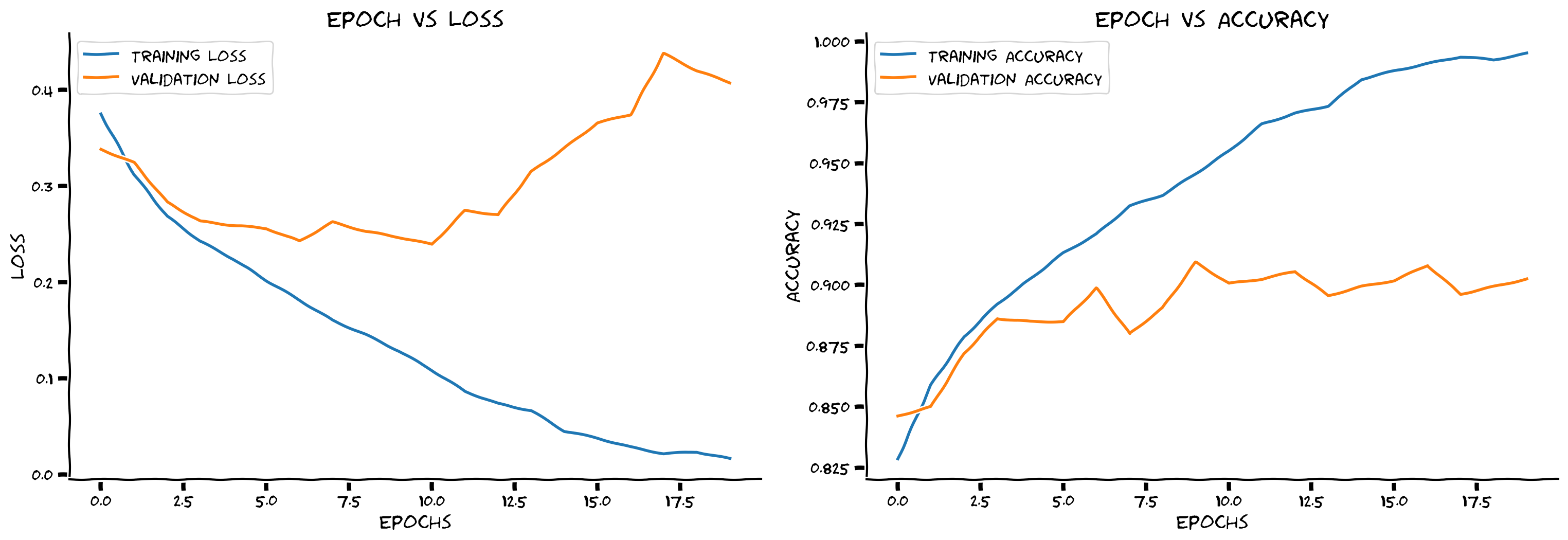
# @title Submit your feedback
content_review(f"{feedback_prefix}_Code_the_training_loop_Bonus_Exercise")
考えてみよう!ボーナス 1: 過学習
このネットワークは過学習していると思いますか?
もしそうなら、これに対抗するために何ができますか?
ヒント: 過学習はトレーニング精度が検証精度を大きく上回るときに起こります。
# @title Submit your feedback
content_review(f"{feedback_prefix}_Overfitting_Bonus_Discussion")
ボーナス 2: 過学習 - 症状と対策
所要時間の目安: 約30分
先週は正則化手法について学びました。以下は以前使ったCNNモデルのコピーです。ここにドロップアウト正則化を追加し、過学習の軽減に効果があるか確認してください。挑戦したい場合はドロップアウト以外の手法も試してみてください。
ボーナス 2.1: 正則化
コーディング演習 ボーナス 2.1: 正則化の追加
さまざまな正則化手法を追加してみてください。自由に追加して試してみましょう!
class FMNIST_Net2(nn.Module):
  """
  Neural Network instance
  """

  def __init__(self, num_classes):
    """
    Initialise parameters of FMNIST_Net2

    Args:
      num_classes: int
        Number of classes

    Returns:
      Nothing
    """
    super(FMNIST_Net2, self).__init__()
    ####################################################################
    # Fill in missing code below (...),
    # then remove or comment the line below to test your function
    raise NotImplementedError("Add regularization layers")
    ####################################################################
    self.conv1 = nn.Conv2d(1, 32, 3, 1)
    self.conv2 = nn.Conv2d(32, 64, 3, 1)
    self.dropout1 = ...
    self.dropout2 = ...
    self.fc1 = nn.Linear(9216, 128)
    self.fc2 = nn.Linear(128, num_classes)

  def forward(self, x):
    """
    Forward pass of FMNIST_Net2

    Args:
      x: torch.tensor
        Input features

    Returns:
      x: torch.tensor
        Output after passing through FMNIST_Net2
    """
    ####################################################################
    # Now add the layers in your forward pass in appropriate order
    # then remove or comment the line below to test your function
    raise NotImplementedError("Add regularization in the forward pass")
    ####################################################################
    x = self.conv1(x)
    x = F.relu(x)
    x = self.conv2(x)
    x = F.relu(x)
    x = F.max_pool2d(x, 2)
    x = ...
    x = torch.flatten(x, 1)
    x = self.fc1(x)
    x = F.relu(x)
    x = ...
    x = self.fc2(x)

    return x


set_seed(SEED)
## Uncomment below to check your code
# net2 = FMNIST_Net2(num_classes=2).to(DEVICE)
# train_loss, train_acc, validation_loss, validation_acc = train(net2, DEVICE, train_loader, validation_loader, 20)
# print(f'Test accuracy is: {test(net2, DEVICE, test_loader)}')
# plot_loss_accuracy(train_loss, train_acc, validation_loss, validation_acc)出力例:
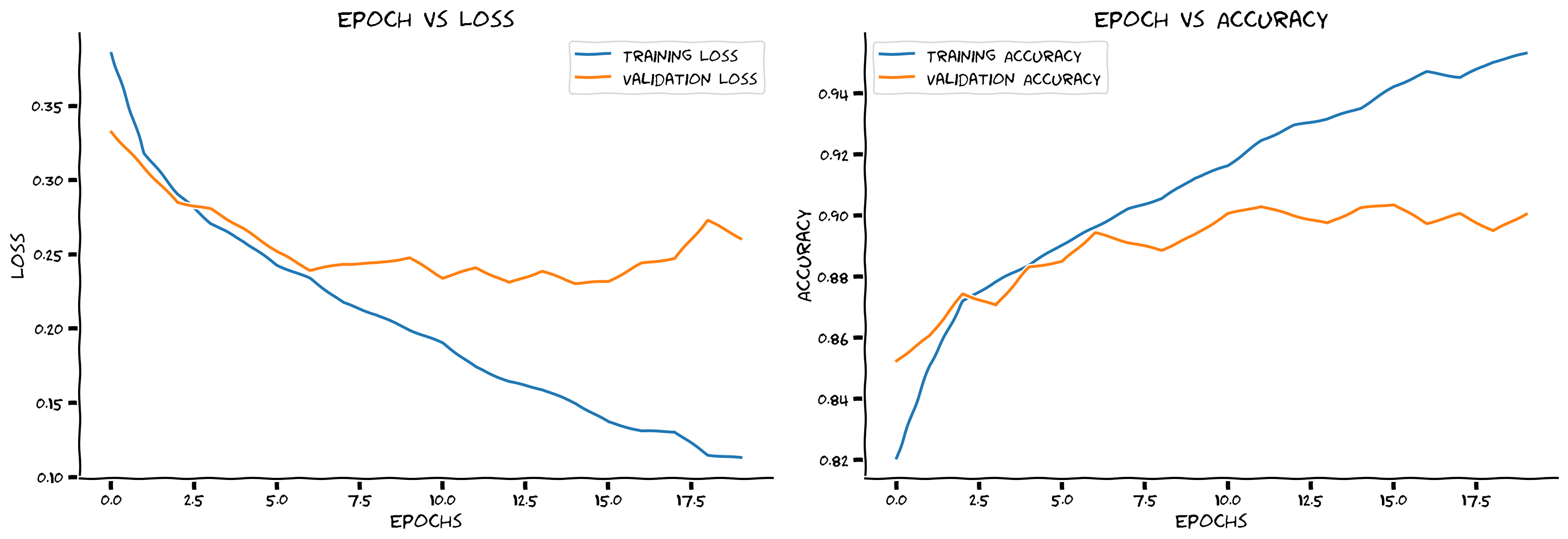
# @title Submit your feedback
content_review(f"{feedback_prefix}_Adding_Regularization_Bonus_Exercise")
考えてみよう!ボーナス 2.1: 正則化
-
正則化を追加する前と比べてトレーニング精度はわずかに下がりましたか?どのくらいの精度まで下げられましたか?
-
なぜ検証精度がトレーニング精度よりも高く始まるのでしょうか?
# @title Submit your feedback
content_review(f"{feedback_prefix}_Adding_Regularization_Bonus_Discussion")
インタラクティブデモ ボーナス 2.1: ドロップアウトの探求
もっと多くのドロップアウトパラメータの組み合わせを試したいけれど時間がない場合は、ここに事前計算済みの組み合わせがあります。スライダーで探索してみてください。
# @markdown *Run this cell to enable the widget*

import io, base64
from ipywidgets import widgets, interactive_output

data = [[0, 0, [0.3495898238046372, 0.2901147632522786, 0.2504794800931469, 0.23571575765914105, 0.21297093365896255, 0.19087818914905508, 0.186408187797729, 0.19487689035211472, 0.16774938120803934, 0.1548648244958926, 0.1390149021382503, 0.10919439224922593, 0.10054351237820501, 0.09900783193594914, 0.08370604479507088, 0.07831853718318521, 0.06859792241866285, 0.06152600247383197, 0.046342475851873885, 0.055123823092992796], [0.83475, 0.8659166666666667, 0.8874166666666666, 0.8913333333333333, 0.8998333333333334, 0.9140833333333334, 0.9178333333333333, 0.9138333333333334, 0.9251666666666667, 0.92975, 0.939, 0.9525833333333333, 0.9548333333333333, 0.9585833333333333, 0.9655833333333333, 0.9661666666666666, 0.9704166666666667, 0.9743333333333334, 0.9808333333333333, 0.9775], [0.334623601436615, 0.2977438402175903, 0.2655304968357086, 0.25506321132183074, 0.2588835284113884, 0.2336345863342285, 0.3029863876104355, 0.240766831189394, 0.2719801160693169, 0.25231350839138034, 0.2500132185220718, 0.26699506521224975, 0.2934862145781517, 0.361227530837059, 0.33196919202804565, 0.36985905408859254, 0.4042587959766388, 0.3716402840614319, 0.3707024946808815, 0.4652537405490875], [0.866875, 0.851875, 0.8775, 0.889375, 0.881875, 0.900625, 0.85, 0.898125, 0.885625, 0.876875, 0.899375, 0.90625, 0.89875, 0.87, 0.898125, 0.884375, 0.874375, 0.89375, 0.903125, 0.890625]], [0, 0.25, [0.35404509995528993, 0.30616586227366266, 0.2872369573946963, 0.27564131199045383, 0.25969504263806853, 0.24728168408445855, 0.23505379509260046, 0.21552803914280647, 0.209761732277718, 0.19977611067526518, 0.19632092922767427, 0.18672360206379535, 0.16564940239124476, 0.1654047035671612, 0.1684555298985636, 0.1627526102349796, 0.13878319327263755, 0.12881529055773577, 0.12628930977525862, 0.11346105090837846], [0.8324166666666667, 0.8604166666666667, 0.8680833333333333, 0.8728333333333333, 0.8829166666666667, 0.88625, 0.89425, 0.90125, 0.9015833333333333, 0.90925, 0.9114166666666667, 0.917, 0.9268333333333333, 0.92475, 0.921, 0.9255833333333333, 0.9385, 0.9428333333333333, 0.9424166666666667, 0.9484166666666667], [0.3533937376737595, 0.29569859683513644, 0.27531551957130435, 0.2576177391409874, 0.26947550356388095, 0.25361743807792664, 0.2527468180656433, 0.24179009914398195, 0.28664454460144045, 0.23347773611545564, 0.24672816634178163, 0.27822364538908007, 0.2380720081925392, 0.24426509588956832, 0.2443918392062187, 0.24207917481660843, 0.2519641682505608, 0.3075403380393982, 0.2798181238770485, 0.26709021866321564], [0.826875, 0.87, 0.870625, 0.8875, 0.883125, 0.88625, 0.891875, 0.891875, 0.890625, 0.903125, 0.89375, 0.885625, 0.903125, 0.888125, 0.899375, 0.898125, 0.905, 0.905625, 0.898125, 0.901875]], [0, 0.5, [0.39775496332886373, 0.33771887778284704, 0.321900939132939, 0.3079229625774191, 0.304149763301966, 0.28249239723416086, 0.2861261191044716, 0.27356165798103554, 0.2654648520686525, 0.2697350280557541, 0.25354846321204877, 0.24612889034633942, 0.23482802549892284, 0.2389904112416379, 0.23742155821875055, 0.232423192127905, 0.22337309338469455, 0.2141852991932884, 0.20677659985549907, 0.19355326712607068], [0.8155, 0.83625, 0.8481666666666666, 0.8530833333333333, 0.8571666666666666, 0.86775, 0.8623333333333333, 0.8711666666666666, 0.8748333333333334, 0.8685833333333334, 0.8785, 0.8804166666666666, 0.8835833333333334, 0.8840833333333333, 0.88875, 0.8919166666666667, 0.8946666666666667, 0.8960833333333333, 0.906, 0.9063333333333333], [0.3430288594961166, 0.4062050700187683, 0.29745822548866274, 0.27728439271450045, 0.28092808067798614, 0.2577864158153534, 0.2651400637626648, 0.25632822573184966, 0.3082498562335968, 0.2812121778726578, 0.26345942318439486, 0.2577408078312874, 0.25757989794015884, 0.26434457510709763, 0.24917411386966706, 0.27261342853307724, 0.2445397639274597, 0.26001051396131514, 0.24147838801145555, 0.2471102523803711], [0.82875, 0.795625, 0.87, 0.87375, 0.865625, 0.8825, 0.8825, 0.87625, 0.848125, 0.87875, 0.8675, 0.889375, 0.8925, 0.866875, 0.87375, 0.87125, 0.895625, 0.90375, 0.90125, 0.88625]], [0, 0.75, [0.4454924576777093, 0.43416607585993217, 0.42200265769311723, 0.40520024616667566, 0.41137005166804536, 0.404100904280835, 0.40118067664034823, 0.40139733080534223, 0.3797615355158106, 0.3596332479030528, 0.3600061919460905, 0.3554147962242999, 0.34480382890460337, 0.3329520877054397, 0.33164913056695716, 0.31860941466181836, 0.30702565340919696, 0.30605297186907304, 0.2953788426486736, 0.2877389984403519], [0.7788333333333334, 0.7825, 0.7854166666666667, 0.7916666666666666, 0.7885, 0.7833333333333333, 0.7923333333333333, 0.79525, 0.805, 0.81475, 0.8161666666666667, 0.8188333333333333, 0.817, 0.8266666666666667, 0.82225, 0.8360833333333333, 0.8456666666666667, 0.8430833333333333, 0.8491666666666666, 0.8486666666666667], [0.3507828885316849, 0.3337512403726578, 0.34320746660232543, 0.3476085543632507, 0.3326113569736481, 0.33033264458179473, 0.32014619171619413, 0.3182142299413681, 0.30076164126396177, 0.3263852882385254, 0.27597591280937195, 0.29062016785144806, 0.2765174686908722, 0.269492534995079, 0.2679423809051514, 0.2691828978061676, 0.2726386785507202, 0.2541181230545044, 0.2580208206176758, 0.26315389811992645], [0.839375, 0.843125, 0.823125, 0.821875, 0.81875, 0.819375, 0.8225, 0.826875, 0.835625, 0.865, 0.868125, 0.855625, 0.868125, 0.884375, 0.883125, 0.875, 0.87375, 0.883125, 0.8975, 0.885]], [0.25, 0, [0.34561181647029326, 0.2834314257699124, 0.2583787844298368, 0.23892096465730922, 0.23207981773513428, 0.20245029634617745, 0.183908417583146, 0.17489413774393975, 0.17696723581707857, 0.15615438255778652, 0.14469048382833283, 0.12424647461305907, 0.11314761043189371, 0.11249036608422373, 0.10725672634199579, 0.09081190969160896, 0.0942245383271353, 0.08525650047677312, 0.06622548752583246, 0.06039895973307021], [0.8356666666666667, 0.8675833333333334, 0.88175, 0.8933333333333333, 0.8975833333333333, 0.91175, 0.91825, 0.9249166666666667, 0.9238333333333333, 0.9305, 0.938, 0.9465833333333333, 0.9525833333333333, 0.9539166666666666, 0.9555, 0.9615, 0.9606666666666667, 0.96275, 0.9725, 0.9764166666666667], [0.31630186855792997, 0.2702121251821518, 0.2915778249502182, 0.26050266206264494, 0.27837209939956664, 0.24276352763175965, 0.3567117482423782, 0.2752074319124222, 0.2423130339384079, 0.2565067422389984, 0.28710135877132414, 0.266545415520668, 0.31818037331104276, 0.28757534325122835, 0.2777567034959793, 0.2998969575762749, 0.3292293107509613, 0.30775387287139894, 0.32681577146053314, 0.44882203072309496], [0.85375, 0.879375, 0.875625, 0.89, 0.86125, 0.884375, 0.851875, 0.8875, 0.89625, 0.875625, 0.8675, 0.895, 0.888125, 0.89125, 0.889375, 0.880625, 0.87875, 0.8875, 0.894375, 0.891875]], [0.25, 0.25, [0.35970850011452715, 0.31336131549261986, 0.2881505932421126, 0.2732012960267194, 0.26232245425753137, 0.2490472443639598, 0.24866499093935845, 0.22930880945096624, 0.21745950407645803, 0.20700296882460725, 0.197304340356842, 0.20665066804182022, 0.19864868348900308, 0.184807124210799, 0.1684703354703936, 0.17377675851767369, 0.16638460063791655, 0.15944768343754906, 0.14876513817208878, 0.1388207479835825], [0.83375, 0.85175, 0.86725, 0.8719166666666667, 0.8761666666666666, 0.8865833333333333, 0.88275, 0.8956666666666667, 0.8995833333333333, 0.9034166666666666, 0.90825, 0.9043333333333333, 0.9093333333333333, 0.9145, 0.9196666666666666, 0.9196666666666666, 0.9216666666666666, 0.9273333333333333, 0.9299166666666666, 0.93675], [0.3166788029670715, 0.28422485530376435, 0.38055971562862395, 0.2586472672224045, 0.2588653892278671, 0.27983254253864287, 0.25693483114242555, 0.26412731170654297, 0.2733065390586853, 0.24399636536836625, 0.24481021404266357, 0.2689305514097214, 0.2527604129910469, 0.24829535871744157, 0.2654112687706947, 0.23074268400669098, 0.24625462979078294, 0.26423920392990113, 0.25540480852127073, 0.25536185175180437], [0.856875, 0.86625, 0.815, 0.8825, 0.88125, 0.875625, 0.89, 0.8775, 0.870625, 0.895, 0.8975, 0.87375, 0.88625, 0.89125, 0.903125, 0.9, 0.893125, 0.89, 0.8925, 0.899375]], [0.25, 0.5, [0.3975753842040579, 0.34884724409339274, 0.3296900932142075, 0.3150389680361494, 0.31285368667003954, 0.30415422033439293, 0.29553352716438314, 0.289314468094009, 0.2806722329969102, 0.2724469883486311, 0.26634286379719035, 0.2645016222241077, 0.2619251853766594, 0.2551752221473354, 0.26411766035759704, 0.24515971153023394, 0.2390686312412962, 0.23573122312255362, 0.221005061562074, 0.22358600648635246], [0.8106666666666666, 0.8286666666666667, 0.844, 0.8513333333333334, 0.84975, 0.8570833333333333, 0.8624166666666667, 0.8626666666666667, 0.866, 0.8706666666666667, 0.8738333333333334, 0.8748333333333334, 0.8778333333333334, 0.8798333333333334, 0.87375, 0.8865, 0.8898333333333334, 0.8885833333333333, 0.8991666666666667, 0.8968333333333334], [0.3597823417186737, 0.31115993797779085, 0.29929635107517244, 0.2986589139699936, 0.2938830828666687, 0.28118040919303894, 0.2711684626340866, 0.2844697123765945, 0.26613601863384245, 0.2783134698867798, 0.2540236383676529, 0.25821100890636445, 0.2618845862150192, 0.2554920208454132, 0.26543013513088226, 0.24074569433927537, 0.26475649774074556, 0.25578504264354707, 0.2648500043153763, 0.25700133621692656], [0.825, 0.8375, 0.85875, 0.855625, 0.861875, 0.868125, 0.875, 0.85375, 0.886875, 0.86375, 0.88375, 0.885625, 0.875625, 0.87375, 0.8875, 0.895, 0.874375, 0.89125, 0.88625, 0.895625]], [0.25, 0.75, [0.4584837538447786, 0.4506375778545725, 0.4378386567089152, 0.4066803843734112, 0.3897064097542712, 0.3855383962868376, 0.39160584618753574, 0.3731403942120836, 0.37915910170116324, 0.36966170814443144, 0.35735995298687445, 0.35630573094525236, 0.346426092167484, 0.34040802899510303, 0.32829743726773464, 0.3284692421872565, 0.3186114077713895, 0.32295761503120685, 0.3201326223764014, 0.30581602454185486], [0.7803333333333333, 0.7709166666666667, 0.7723333333333333, 0.7850833333333334, 0.7885, 0.7903333333333333, 0.7986666666666666, 0.805, 0.8011666666666667, 0.8068333333333333, 0.8095833333333333, 0.8226666666666667, 0.8285, 0.83125, 0.8369166666666666, 0.8395, 0.8441666666666666, 0.8393333333333334, 0.8490833333333333, 0.8546666666666667], [0.43526833415031435, 0.3598956459760666, 0.3492005372047424, 0.33501910269260404, 0.31689528703689573, 0.3113307124376297, 0.32388085544109346, 0.3084335786104202, 0.3013568025827408, 0.28992725372314454, 0.28726822674274444, 0.26945948660373686, 0.276592333316803, 0.27462401330471037, 0.27574350595474245, 0.2710308712720871, 0.2702724140882492, 0.27323003828525544, 0.25551479041576386, 0.26488787233829497], [0.808125, 0.81625, 0.805, 0.8325, 0.846875, 0.835625, 0.850625, 0.838125, 0.836875, 0.861875, 0.85375, 0.866875, 0.858125, 0.8825, 0.879375, 0.874375, 0.874375, 0.886875, 0.883125, 0.86875]], [0.5, 0, [0.3579516930783049, 0.29596046564426826, 0.2779693031247626, 0.2563994538356015, 0.24771526356802342, 0.2324555875693864, 0.2139121579362991, 0.20474095547452886, 0.19138856208387842, 0.18883306279461434, 0.1763652620757831, 0.1698919345248253, 0.16033914366221808, 0.1557997044651432, 0.1432509447467771, 0.13817814606776896, 0.12609625801919622, 0.11830132696381275, 0.11182412960903441, 0.112559904720872], [0.8314166666666667, 0.8611666666666666, 0.8736666666666667, 0.8800833333333333, 0.885, 0.8944166666666666, 0.9036666666666666, 0.9090833333333334, 0.9193333333333333, 0.9161666666666667, 0.92225, 0.9255, 0.93075, 0.93225, 0.939, 0.9414166666666667, 0.94375, 0.9485833333333333, 0.9535833333333333, 0.9524166666666667], [0.30677567660808563, 0.32954772651195524, 0.25747098088264464, 0.2736126834154129, 0.2561805549263954, 0.23671718776226044, 0.24553639352321624, 0.2338863667845726, 0.24586652517318724, 0.23423030972480774, 0.26579618513584136, 0.2781539523601532, 0.27084136098623274, 0.23948652744293214, 0.26023868829011915, 0.2419952344894409, 0.2511997854709625, 0.23935708701610564, 0.2701922015845776, 0.27307246536016466], [0.870625, 0.855625, 0.886875, 0.875625, 0.878125, 0.8925, 0.885, 0.890625, 0.876875, 0.896875, 0.881875, 0.8875, 0.89, 0.898125, 0.896875, 0.89, 0.89875, 0.904375, 0.906875, 0.894375]], [0.5, 0.25, [0.3712943946903056, 0.3198322071594761, 0.29978102302931725, 0.295274139798068, 0.2861913934032968, 0.27165328782606635, 0.25972246442069397, 0.2543164194819141, 0.24795781916126292, 0.24630710007028378, 0.23296909834793272, 0.23382153587931015, 0.2239028559799524, 0.21443849290780564, 0.2149274461367663, 0.20642021417300752, 0.19801520536396097, 0.1978839404009124, 0.19118623847657062, 0.18144798041024107], [0.8235833333333333, 0.8538333333333333, 0.8604166666666667, 0.86075, 0.8664166666666666, 0.8754166666666666, 0.8799166666666667, 0.8815833333333334, 0.88725, 0.8848333333333334, 0.8936666666666667, 0.8935, 0.895, 0.8995, 0.89625, 0.9068333333333334, 0.9098333333333334, 0.9120833333333334, 0.91375, 0.9175833333333333], [0.3184810388088226, 0.2948088157176971, 0.29438531696796416, 0.27669853866100313, 0.2634278678894043, 0.25847582578659056, 0.2500907778739929, 0.2538330048322678, 0.25127841770648957, 0.2519759064912796, 0.2455715072154999, 0.2437664610147476, 0.259639236330986, 0.24515749186277389, 0.2553828465938568, 0.2324645048379898, 0.24492083072662355, 0.24482838332653045, 0.23327024638652802, 0.2520161652565002], [0.855, 0.865, 0.8525, 0.856875, 0.876875, 0.88125, 0.8825, 0.8875, 0.8925, 0.8925, 0.88875, 0.889375, 0.87375, 0.895, 0.889375, 0.90625, 0.883125, 0.895, 0.899375, 0.901875]], [0.5, 0.5, [0.40442772225496615, 0.36662670541951, 0.355034276367502, 0.3396551510755052, 0.3378269396563794, 0.32084332002287214, 0.31314464951766297, 0.2982726935693558, 0.2885229691387491, 0.2888992782285873, 0.2893476904706752, 0.281817957996688, 0.2771622718490185, 0.2693793097550565, 0.2617615883416952, 0.2657115764995205, 0.25631817549150043, 0.24793559907281654, 0.2538738044652533, 0.23912971732305718], [0.8093333333333333, 0.82825, 0.8341666666666666, 0.84525, 0.84525, 0.8515, 0.8583333333333333, 0.8626666666666667, 0.8688333333333333, 0.8685, 0.8689166666666667, 0.8693333333333333, 0.8711666666666666, 0.8766666666666667, 0.88275, 0.88175, 0.8839166666666667, 0.8866666666666667, 0.8839166666666667, 0.8929166666666667], [0.38392188608646394, 0.3653419762849808, 0.3050421380996704, 0.30614266455173494, 0.2937217426300049, 0.30008585572242735, 0.2794034606218338, 0.27541795969009397, 0.31378355383872986, 0.2670704126358032, 0.26745485186576845, 0.2471194839477539, 0.26509816259145735, 0.25458798944950106, 0.2481587851047516, 0.25591064751148224, 0.2596563971042633, 0.2569611769914627, 0.2435744071006775, 0.2507249677181244], [0.820625, 0.846875, 0.856875, 0.868125, 0.860625, 0.87125, 0.86625, 0.87375, 0.865625, 0.87875, 0.878125, 0.889375, 0.87875, 0.886875, 0.89125, 0.89, 0.87375, 0.884375, 0.88875, 0.89375]], [0.5, 0.75, [0.46106574311852455, 0.4519433615372536, 0.4446939624687459, 0.4284856241751224, 0.4527993325857406, 0.4220876024758562, 0.40969764266876463, 0.39233948219012704, 0.42498463344700793, 0.3869199570506177, 0.38021832910623954, 0.3855376149270129, 0.3721433773319772, 0.3662295250340979, 0.3629763710530514, 0.358500304691335, 0.3490118366131123, 0.34879197790584665, 0.33399240054348683, 0.3347948451149971], [0.7866666666666666, 0.7865, 0.784, 0.79375, 0.7755833333333333, 0.79125, 0.7973333333333333, 0.8085833333333333, 0.7913333333333333, 0.8125833333333333, 0.81675, 0.812, 0.8173333333333334, 0.8235833333333333, 0.831, 0.8306666666666667, 0.8353333333333334, 0.8320833333333333, 0.84375, 0.8410833333333333], [0.35159709095954894, 0.3579048192501068, 0.3501501774787903, 0.33594816565513613, 0.3741619431972504, 0.34183687329292295, 0.3353554099798203, 0.32617265462875367, 0.3640907108783722, 0.33187183618545535, 0.32401839792728426, 0.30536725163459777, 0.31303414940834046, 0.2893040508031845, 0.3063929396867752, 0.2909839802980423, 0.2858921372890472, 0.2850045281648636, 0.28049838364124297, 0.2873564797639847], [0.816875, 0.793125, 0.810625, 0.821875, 0.8175, 0.82, 0.816875, 0.814375, 0.828125, 0.83875, 0.818125, 0.843125, 0.834375, 0.85875, 0.874375, 0.85375, 0.870625, 0.85375, 0.883125, 0.848125]], [0.75, 0, [0.37716902824158366, 0.3260373148195287, 0.3128290904012132, 0.2998493126732238, 0.29384377892030045, 0.2759418967873492, 0.26431119905665834, 0.2577077782455277, 0.25772295725789474, 0.24954422610871335, 0.24065862928933285, 0.23703582263848882, 0.23237684028262787, 0.2200249534575863, 0.22110319957929722, 0.21804759631607126, 0.21419822757548473, 0.19927451733816812, 0.19864692467641323, 0.18966749441274938], [0.8215833333333333, 0.848, 0.8526666666666667, 0.8585, 0.8639166666666667, 0.8716666666666667, 0.8783333333333333, 0.8849166666666667, 0.88325, 0.88325, 0.8918333333333334, 0.8913333333333333, 0.896, 0.9010833333333333, 0.8996666666666666, 0.9016666666666666, 0.902, 0.9120833333333334, 0.9105833333333333, 0.9160833333333334], [0.3255926352739334, 0.3397491586208343, 0.3148202610015869, 0.30447013437747955, 0.27427292466163633, 0.2607581865787506, 0.2583494257926941, 0.24150457441806794, 0.24839721441268922, 0.24157819360494615, 0.24594406485557557, 0.2547012311220169, 0.24132476687431337, 0.2433958488702774, 0.2358475297689438, 0.24675665378570558, 0.23343635857105255, 0.22841362684965133, 0.2247604575753212, 0.24281086921691894], [0.85125, 0.85125, 0.853125, 0.851875, 0.876875, 0.87875, 0.883125, 0.888125, 0.89, 0.888125, 0.88375, 0.86625, 0.88375, 0.888125, 0.898125, 0.88875, 0.896875, 0.894375, 0.899375, 0.88625]], [0.75, 0.25, [0.3795942336796446, 0.33614943612446174, 0.3235826115024851, 0.3267444484728448, 0.30353531146303137, 0.29750882636042353, 0.2964640334248543, 0.28714796314214136, 0.2744278162717819, 0.27310871372514584, 0.2624819800257683, 0.2579742945889209, 0.25963644726954876, 0.25635017161356644, 0.2501001837960583, 0.24249463702769988, 0.23696896695393196, 0.23254455582417072, 0.22419108628751117, 0.22851746232110134], [0.8204166666666667, 0.839, 0.847, 0.8506666666666667, 0.8571666666666666, 0.8635, 0.8639166666666667, 0.8711666666666666, 0.8711666666666666, 0.87475, 0.87875, 0.87925, 0.8805833333333334, 0.8845, 0.88675, 0.8908333333333334, 0.8926666666666667, 0.89525, 0.8985, 0.8955833333333333], [0.3383863967657089, 0.31120560944080355, 0.32110977828502657, 0.3080899566411972, 0.2866462391614914, 0.27701647162437437, 0.29040718913078306, 0.2702513742446899, 0.2590403389930725, 0.26199558019638064, 0.26484714448451996, 0.2940529054403305, 0.2654808533191681, 0.25154681205749513, 0.26637687146663663, 0.24435366928577423, 0.24174826145172118, 0.2444209086894989, 0.247626873254776, 0.24192263156175614], [0.843125, 0.8575, 0.86, 0.86375, 0.87, 0.875625, 0.865, 0.88, 0.879375, 0.885, 0.888125, 0.85625, 0.87625, 0.88375, 0.879375, 0.888125, 0.8875, 0.886875, 0.8825, 0.8925]], [0.75, 0.5, [0.41032169133107715, 0.37122817583223605, 0.35897897873470125, 0.3438001747064768, 0.33858899811797954, 0.3389760729797343, 0.32536247420184156, 0.3152934226425404, 0.30936657058748795, 0.3078679118226183, 0.30974164977669716, 0.30031369174731537, 0.29489042173991814, 0.28921707251921613, 0.28369594476324445, 0.2849519875772456, 0.27076949349584734, 0.26930386248104116, 0.26349931491657774, 0.26431971300948176], [0.8086666666666666, 0.82875, 0.8284166666666667, 0.8381666666666666, 0.837, 0.8389166666666666, 0.8490833333333333, 0.8488333333333333, 0.8533333333333334, 0.8551666666666666, 0.8509166666666667, 0.8615, 0.8628333333333333, 0.86225, 0.8715, 0.86775, 0.8748333333333334, 0.8719166666666667, 0.8814166666666666, 0.8835], [0.3464747530221939, 0.3193131250143051, 0.3464068531990051, 0.3129056388139725, 0.3131117367744446, 0.30689118325710296, 0.2929005026817322, 0.3131696957349777, 0.302835636138916, 0.27934255003929137, 0.300513002872467, 0.26962003886699676, 0.2676294481754303, 0.26430738389492037, 0.2525753951072693, 0.2508367341756821, 0.25303518533706665, 0.24774718701839446, 0.24518848478794097, 0.26084545016288757], [0.8225, 0.85375, 0.849375, 0.853125, 0.85875, 0.848125, 0.856875, 0.8575, 0.87, 0.869375, 0.863125, 0.886875, 0.8725, 0.878125, 0.894375, 0.888125, 0.8875, 0.89125, 0.88875, 0.86875]], [0.75, 0.75, [0.4765880586619073, 0.4503744399928032, 0.4249279998401378, 0.42333967214886176, 0.4236916420941657, 0.4269233151002133, 0.4192506206479478, 0.41413671872083174, 0.41084911515738104, 0.389948022413127, 0.39566395788433706, 0.3741930383951106, 0.3794517093040842, 0.3692300356131919, 0.3640432547223061, 0.3608953575504587, 0.3419572095129084, 0.34907091543712515, 0.33601277535583113, 0.3408893179544743], [0.77625, 0.7823333333333333, 0.7916666666666666, 0.80075, 0.7973333333333333, 0.7810833333333334, 0.7928333333333333, 0.7930833333333334, 0.7951666666666667, 0.8015833333333333, 0.8000833333333334, 0.8126666666666666, 0.811, 0.81775, 0.8236666666666667, 0.8215, 0.8305833333333333, 0.8251666666666667, 0.8299166666666666, 0.836], [0.3674533206224442, 0.36733597874641416, 0.35894496202468873, 0.3514183223247528, 0.35345671892166136, 0.36494161546230314, 0.35217500329017637, 0.3447349113225937, 0.34697150766849516, 0.36931039452552794, 0.3350031852722168, 0.3416145300865173, 0.32389605045318604, 0.3109715062379837, 0.3322615468502045, 0.327584428191185, 0.31910278856754304, 0.311815539598465, 0.2950947880744934, 0.2948034608364105], [0.808125, 0.789375, 0.826875, 0.821875, 0.81375, 0.804375, 0.80625, 0.83, 0.820625, 0.848125, 0.816875, 0.8125, 0.83, 0.84625, 0.824375, 0.828125, 0.825625, 0.840625, 0.8475, 0.844375]]]
data = [[0, 0, [0.400307985173582, 0.2597426520640662, 0.20706942731312025, 0.17091670006251475, 0.13984850759524653, 0.11444453444522518, 0.0929887340481538, 0.07584588486117436, 0.06030314570384176, 0.04997897459031356, 0.037156337104278056, 0.02793900864590992, 0.02030197833807442, 0.01789472087045391, 0.0175876492686666, 0.019220354652448274, 0.013543135874294319, 0.006956856955481477, 0.0024507183060002227, 0.00206579088377317], [0.8547833333333333, 0.9049, 0.9241666666666667, 0.9360166666666667, 0.94695, 0.9585833333333333, 0.9658666666666667, 0.9723166666666667, 0.9780333333333333, 0.9820166666666666, 0.9868, 0.9906666666666667, 0.9936833333333334, 0.9941333333333333, 0.99405, 0.9932833333333333, 0.9960666666666667, 0.9979666666666667, 0.9996666666666667, 0.9995666666666667], [0.36797549843788147, 0.2586278670430183, 0.24208260095119477, 0.24353929474949837, 0.24164094921946525, 0.2638056704550982, 0.2579395814836025, 0.27675500786304474, 0.2851512663513422, 0.30380481338500975, 0.3235128371268511, 0.3284085538983345, 0.3443841063082218, 0.41086878085136413, 0.457796107493341, 0.4356938077956438, 0.4109785168170929, 0.4433729724138975, 0.4688420155197382, 0.4773445381522179], [0.87, 0.908375, 0.91475, 0.915125, 0.91525, 0.91725, 0.924875, 0.91975, 0.922375, 0.92025, 0.920375, 0.924875, 0.9235, 0.918125, 0.91525, 0.918875, 0.923625, 0.9235, 0.92625, 0.925]], [0, 0.25, [0.4710115425463424, 0.3166707545550647, 0.25890692547440275, 0.22350736999753187, 0.19296910860009794, 0.17304379170113154, 0.15315235079105285, 0.13728606270383925, 0.12178339355929034, 0.10961619754736898, 0.10074329449495337, 0.08793247367408294, 0.07651288138686625, 0.06934997136779089, 0.06243234033510685, 0.056774082654433795, 0.05116950291028218, 0.04961718403588313, 0.04289388027836952, 0.040430180404756245], [0.8289666666666666, 0.8851833333333333, 0.9045166666666666, 0.9167666666666666, 0.9294166666666667, 0.93545, 0.94275, 0.9486666666666667, 0.95365, 0.95855, 0.9618833333333333, 0.9667, 0.9717666666666667, 0.9745833333333334, 0.9765833333333334, 0.9793, 0.9809833333333333, 0.9820333333333333, 0.9839166666666667, 0.9849166666666667], [0.3629846270084381, 0.31240448981523516, 0.24729759228229523, 0.2697310926616192, 0.24718070650100707, 0.23403583562374114, 0.2295891786813736, 0.22117181441187858, 0.2475375788807869, 0.23771390727162361, 0.2562992911040783, 0.25533875498175623, 0.27057862806320193, 0.2820998176634312, 0.29471745146811007, 0.2795617451965809, 0.3008101430237293, 0.28815430629253386, 0.31814645100384953, 0.3106237706840038], [0.874125, 0.88875, 0.908875, 0.9045, 0.9145, 0.918125, 0.919375, 0.9245, 0.91975, 0.926, 0.923625, 0.925875, 0.92475, 0.926375, 0.925125, 0.92525, 0.924625, 0.930875, 0.924875, 0.926625]], [0, 0.5, [0.6091368444629316, 0.40709905083309106, 0.33330900164873106, 0.29541655938063605, 0.26824146830864043, 0.24633059249535552, 0.22803501166832219, 0.21262132842689435, 0.20038021789160745, 0.18430457027680647, 0.1744787511763288, 0.165271017740149, 0.15522625095554507, 0.1432937567076608, 0.13617747858651222, 0.12876031456241158, 0.12141566201230325, 0.11405601029369686, 0.11116664642408522, 0.10308189516060992], [0.7803833333333333, 0.8559166666666667, 0.8823, 0.89505, 0.9027333333333334, 0.9099166666666667, 0.9162333333333333, 0.9224833333333333, 0.9243166666666667, 0.9321, 0.9345833333333333, 0.9375333333333333, 0.9418833333333333, 0.9456666666666667, 0.9482333333333334, 0.9513666666666667, 0.9527333333333333, 0.9559, 0.9576166666666667, 0.9611], [0.36491659212112426, 0.29200539910793305, 0.2840233483910561, 0.2591339669823646, 0.24114771646261215, 0.2436459481716156, 0.2374294084906578, 0.24284198743104934, 0.22679156363010405, 0.2229055170416832, 0.21932773572206496, 0.23045065227150918, 0.23631879675388337, 0.22048399156332016, 0.2563135535418987, 0.2494968646839261, 0.24099056956171988, 0.23974315640330315, 0.24684958010911942, 0.25887142738699914], [0.8665, 0.8925, 0.897, 0.907375, 0.914125, 0.9125, 0.913875, 0.911875, 0.921125, 0.922625, 0.923375, 0.924125, 0.922625, 0.926, 0.915625, 0.926125, 0.932625, 0.927875, 0.93, 0.92525]], [0, 0.75, [1.187068938827718, 0.9080034740316842, 0.6863665148329887, 0.5706229420867301, 0.5069490017921432, 0.46316734996876485, 0.42913920047885573, 0.4107565824855874, 0.3908677859061054, 0.37283689377785745, 0.3606657798388111, 0.353545261082301, 0.34009441143986, 0.3239413740506559, 0.3193119444620253, 0.31045137204404577, 0.3003838519091164, 0.29092520530194615, 0.28635713599447504, 0.2760026559138349], [0.5551333333333334, 0.6467, 0.7338666666666667, 0.7841333333333333, 0.8128, 0.82845, 0.8430833333333333, 0.8501666666666666, 0.8580833333333333, 0.8646166666666667, 0.8667666666666667, 0.8709833333333333, 0.8766166666666667, 0.8816666666666667, 0.8812, 0.88465, 0.8898833333333334, 0.8934666666666666, 0.8940833333333333, 0.8977666666666667], [0.6463955206871033, 0.5193838343620301, 0.4155286856889725, 0.3316091845035553, 0.3148408111333847, 0.29354524302482604, 0.2875490103960037, 0.26903486740589144, 0.27737221759557723, 0.262776792883873, 0.25498255288600924, 0.2390553195178509, 0.24918611392378806, 0.23830307483673097, 0.23538302001357078, 0.24996423116326333, 0.2464654156267643, 0.24081429636478424, 0.23204647853970528, 0.23771219885349273], [0.763875, 0.81925, 0.8685, 0.8885, 0.8895, 0.895625, 0.902, 0.904125, 0.906125, 0.908, 0.909375, 0.9145, 0.916125, 0.9175, 0.91875, 0.91425, 0.915375, 0.918875, 0.91975, 0.91825]], [0.25, 0, [0.4140813298491654, 0.27481235485118843, 0.22397600941614174, 0.1890777693286951, 0.16538111197112848, 0.1448796250478132, 0.12440053254032313, 0.10817898457734855, 0.09634132136696025, 0.08548538653410352, 0.07339220296349257, 0.06470446296305314, 0.060030178171393875, 0.053294485403614034, 0.04429284706704323, 0.04014099264770115, 0.03974721442450951, 0.03304463665041803, 0.02955428938137994, 0.026940144761875052], [0.8496666666666667, 0.8982666666666667, 0.9162166666666667, 0.9292166666666667, 0.93805, 0.9457666666666666, 0.9534333333333334, 0.9596, 0.9645833333333333, 0.9679, 0.9726166666666667, 0.9761666666666666, 0.9775, 0.9800166666666666, 0.9842, 0.9855333333333334, 0.9857, 0.98805, 0.9895666666666667, 0.9905833333333334], [0.3327465409040451, 0.27738857254385946, 0.23834018683433533, 0.24359044748544692, 0.23630736249685289, 0.26239568686485293, 0.23089197066426276, 0.23183160039782524, 0.2287161501646042, 0.23795067170262338, 0.2680365410447121, 0.28079107534885406, 0.2745736412107945, 0.27641161236166956, 0.2967236565724015, 0.29836027943715454, 0.28526886811852453, 0.3188628684282303, 0.3159900237545371, 0.33990017675608397], [0.876875, 0.899875, 0.918125, 0.9105, 0.918125, 0.91, 0.92075, 0.922625, 0.924, 0.921, 0.920875, 0.921, 0.9285, 0.927625, 0.9265, 0.927375, 0.925875, 0.927, 0.92575, 0.925875]], [0.25, 0.25, [0.48859380523978013, 0.3269256727337075, 0.275135099903734, 0.24039912359244914, 0.21368402032566858, 0.19328243048317523, 0.17890911489359732, 0.16624130663682402, 0.15215728174088827, 0.1416037013468299, 0.13273427299440288, 0.12227611260405227, 0.11463099068699917, 0.10616964906720179, 0.09988978996809357, 0.09424899211093815, 0.08670466838887077, 0.0835973875783781, 0.0778748192367698, 0.07327510508696741], [0.82055, 0.8806666666666667, 0.9004333333333333, 0.9117333333333333, 0.9206333333333333, 0.92785, 0.9333, 0.9384166666666667, 0.9430333333333333, 0.9471833333333334, 0.95055, 0.9540166666666666, 0.9568833333333333, 0.9601666666666666, 0.9620333333333333, 0.9652, 0.9676833333333333, 0.9682666666666667, 0.9706, 0.9724333333333334], [0.34025013536214826, 0.29788709819316866, 0.2680273652672768, 0.2463292105793953, 0.23471139985322953, 0.22580294385552407, 0.21676637730002404, 0.20925517010688782, 0.23552959233522416, 0.21975916308164598, 0.23494828915596008, 0.21611644634604454, 0.22251244640350343, 0.22066593673825263, 0.2214409472346306, 0.22849382662773132, 0.24493269926309585, 0.2397777333110571, 0.23578458192944526, 0.2563280282020569], [0.870875, 0.8875, 0.900375, 0.906625, 0.9145, 0.921125, 0.92125, 0.92425, 0.916, 0.923125, 0.920375, 0.92675, 0.92575, 0.924875, 0.925, 0.924875, 0.922875, 0.931125, 0.932375, 0.929]], [0.25, 0.5, [0.6104797730917362, 0.42115319246994154, 0.3527538229359874, 0.3136731511446586, 0.2857721160565104, 0.26646374052426197, 0.24732486170523965, 0.23057452346613286, 0.21953405395769743, 0.20952929538100767, 0.19584925043811677, 0.18926965880162044, 0.18003955145856973, 0.17379174885878176, 0.16635702809354644, 0.15807223409366633, 0.1509416516620054, 0.1477138751140758, 0.14028569269798266, 0.13906246528172417], [0.7786833333333333, 0.8482166666666666, 0.8730833333333333, 0.888, 0.8978, 0.9033666666666667, 0.9089166666666667, 0.9147666666666666, 0.91955, 0.9221833333333334, 0.92715, 0.9309666666666667, 0.9334, 0.93495, 0.9376833333333333, 0.9402666666666667, 0.94405, 0.9439166666666666, 0.9466833333333333, 0.9464833333333333], [0.3859497320652008, 0.3124091213941574, 0.28177140313386917, 0.2564259949326515, 0.24969424712657928, 0.23137387067079543, 0.22758139592409135, 0.22978509336709976, 0.2293499847650528, 0.22430640310049058, 0.21563700905442237, 0.21529569518566133, 0.22171301135420798, 0.2105387990772724, 0.21190602815151213, 0.21494245541095733, 0.21312989933788776, 0.20670134457945824, 0.2146600303351879, 0.21474341893941165], [0.86, 0.888, 0.89625, 0.907, 0.908, 0.915, 0.917875, 0.92, 0.921125, 0.917625, 0.924, 0.921875, 0.925875, 0.92575, 0.928125, 0.92775, 0.928625, 0.93075, 0.92975, 0.930375]], [0.25, 0.75, [1.1724896589194789, 0.8803599189911315, 0.692622532690766, 0.5974764075837156, 0.5319996399920124, 0.49373906012028773, 0.4741932853007876, 0.45601858158927483, 0.43706520244892216, 0.4238534729236733, 0.41077356216813454, 0.38932509837882606, 0.3771154705856019, 0.3687882057305719, 0.34927689276937485, 0.3379922736602933, 0.33547254843212393, 0.3263144160448107, 0.31800466419251233, 0.3133781185822446], [0.5631833333333334, 0.6579333333333334, 0.7342166666666666, 0.7765833333333333, 0.8036333333333333, 0.8197166666666666, 0.82755, 0.8320166666666666, 0.8397833333333333, 0.8432666666666667, 0.8519333333333333, 0.85835, 0.86285, 0.8641, 0.87105, 0.8756666666666667, 0.8775166666666666, 0.87965, 0.88255, 0.8832333333333333], [0.5745115535259246, 0.4740168128013611, 0.4092038922309876, 0.345498643040657, 0.32894178831577303, 0.2999964846372604, 0.28456189918518066, 0.28186965006589887, 0.26958267349004744, 0.26703972268104553, 0.2667745503783226, 0.2553461962342262, 0.25764305877685545, 0.2528705199956894, 0.24987997275590895, 0.24210182267427444, 0.2366510547697544, 0.24053962442278862, 0.22825994032621383, 0.2270425768494606], [0.776875, 0.822625, 0.848875, 0.87825, 0.88925, 0.899875, 0.9015, 0.904375, 0.9035, 0.906, 0.906875, 0.91125, 0.907, 0.908625, 0.91175, 0.917125, 0.91675, 0.916125, 0.919875, 0.917625]], [0.5, 0, [0.43062501005145276, 0.29807482149078646, 0.2541527441585623, 0.21918726423338278, 0.1950343672964555, 0.17517360023010387, 0.16213757058244144, 0.14869415854364, 0.13477844860392815, 0.12352272007129848, 0.11392300839184412, 0.10589898744228679, 0.09751250602896692, 0.089864786467088, 0.08516462990539526, 0.07973235945548934, 0.07441158362824137, 0.07053931183896578, 0.06258528833356954, 0.06177985634201014], [0.8429, 0.88905, 0.9052166666666667, 0.9182166666666667, 0.92755, 0.9337666666666666, 0.93835, 0.944, 0.9489333333333333, 0.95365, 0.9565333333333333, 0.9599166666666666, 0.9637833333333333, 0.9659666666666666, 0.9685666666666667, 0.9705, 0.9713666666666667, 0.9738, 0.9770166666666666, 0.9769833333333333], [0.32814766228199005, 0.29447353577613833, 0.25052148789167406, 0.22761481428146363, 0.23280890756845474, 0.23155913531780242, 0.21984874603152274, 0.2166314404308796, 0.2202563073039055, 0.22508277136087418, 0.2237191815972328, 0.2246915928721428, 0.22815296687185765, 0.2254556802213192, 0.2337513281852007, 0.2381753808259964, 0.24798179551959038, 0.24766947883367538, 0.24877363580465317, 0.2518915164768696], [0.879625, 0.89025, 0.907875, 0.916625, 0.91625, 0.91825, 0.920875, 0.923625, 0.922625, 0.923, 0.92575, 0.927125, 0.928625, 0.92625, 0.925375, 0.925625, 0.926375, 0.92475, 0.9255, 0.92675]], [0.5, 0.25, [0.5022556754285847, 0.3545388207554436, 0.2965180559564374, 0.2689443711818917, 0.24340009927622544, 0.22504497168144819, 0.21177587015574167, 0.19926073912507308, 0.18498492261557692, 0.1792394390810273, 0.16716771742809555, 0.16088557891500022, 0.15540826101420022, 0.1471743908549931, 0.14383414784458273, 0.1351151093741311, 0.1312572255915305, 0.12904865093140014, 0.12332957751079918, 0.11934908895072208], [0.8186333333333333, 0.8711666666666666, 0.8905666666666666, 0.9020666666666667, 0.9106333333333333, 0.9169333333333334, 0.9227, 0.9258166666666666, 0.9317, 0.9329666666666667, 0.9384833333333333, 0.9394333333333333, 0.94185, 0.9447666666666666, 0.9449833333333333, 0.9489, 0.9506, 0.9520333333333333, 0.95295, 0.9556833333333333], [0.37072600054740906, 0.2894986196160316, 0.2896255247592926, 0.2553737629055977, 0.2347450014948845, 0.23144772934913635, 0.22532679361104965, 0.2152210614681244, 0.21610748746991157, 0.22872606116533278, 0.22058768355846406, 0.20230921444296837, 0.2118315652012825, 0.20028054055571556, 0.20844366964697839, 0.20884322375059128, 0.21231223946809769, 0.19875787001848222, 0.2072589308321476, 0.22480831852555275], [0.862, 0.894, 0.892375, 0.906375, 0.912625, 0.91375, 0.916875, 0.918875, 0.92125, 0.9185, 0.920375, 0.92825, 0.9255, 0.92925, 0.926875, 0.9285, 0.926375, 0.93075, 0.931125, 0.922875]], [0.5, 0.5, [0.6208003907124879, 0.4341448332582201, 0.3655890760454796, 0.3245583019102179, 0.3000562671722888, 0.2840681741280215, 0.2686156402947679, 0.25843519997844566, 0.24892204790227196, 0.23988707410469493, 0.22968693327770304, 0.22323107979953416, 0.21376596502403714, 0.21353628940340172, 0.208721635311143, 0.20283085862393063, 0.19862186088204892, 0.1939613972542319, 0.18833921627917968, 0.18451892669552933], [0.7769666666666667, 0.8453333333333334, 0.86965, 0.88425, 0.8911, 0.8957666666666667, 0.90125, 0.9056666666666666, 0.9083833333333333, 0.9122666666666667, 0.91455, 0.9176833333333333, 0.92035, 0.9217, 0.9232333333333334, 0.9238333333333333, 0.9270333333333334, 0.9283, 0.93035, 0.9312333333333334], [0.390482270359993, 0.3140819278359413, 0.286346542596817, 0.26530489122867584, 0.25648517191410064, 0.25534764647483826, 0.24066219604015351, 0.22813884472846985, 0.22091108289361, 0.22591463786363603, 0.22548504903912545, 0.21807716876268388, 0.23463654381036758, 0.21917386519908905, 0.2077158398628235, 0.2112607652246952, 0.205703763961792, 0.21748955991864205, 0.20092388433218003, 0.20742826372385026], [0.859125, 0.884375, 0.89225, 0.9035, 0.9045, 0.904875, 0.907875, 0.915375, 0.914875, 0.915375, 0.916375, 0.92075, 0.91575, 0.91825, 0.92375, 0.924, 0.924875, 0.917125, 0.926875, 0.920875]], [0.5, 0.75, [1.1608194957918196, 0.8736483463918222, 0.7270457689632485, 0.6118623841482439, 0.5539627463769302, 0.5169604117872872, 0.4843029365547176, 0.4664089765979537, 0.449539397952399, 0.4308713404481599, 0.4170197155842903, 0.4104185118508746, 0.3983522486299086, 0.3890672579232945, 0.38423672571047535, 0.38125834129512437, 0.36963055836461756, 0.36898326972273116, 0.3608236700328174, 0.35822524538617145], [0.56785, 0.6591833333333333, 0.71765, 0.7660333333333333, 0.7931666666666667, 0.8079666666666667, 0.8198833333333333, 0.8275166666666667, 0.8349833333333333, 0.8422, 0.8473666666666667, 0.8486833333333333, 0.85425, 0.85675, 0.8578666666666667, 0.8603333333333333, 0.8643333333333333, 0.8637833333333333, 0.8684333333333333, 0.8680166666666667], [0.5984484012126923, 0.5152713191509247, 0.42289899206161496, 0.3746640253067017, 0.3369040569067001, 0.32359291434288023, 0.2978636801838875, 0.2998174095153809, 0.2883352539539337, 0.2839300352931023, 0.2775397801399231, 0.2616970262527466, 0.259125192284584, 0.25470315623283385, 0.2535187450051308, 0.2600560383200645, 0.25031394577026367, 0.2547155976295471, 0.23950587111711502, 0.24401323813199996], [0.750875, 0.78025, 0.86225, 0.869875, 0.884875, 0.891625, 0.898875, 0.89275, 0.901875, 0.9005, 0.899875, 0.908375, 0.91125, 0.910375, 0.910375, 0.907, 0.9135, 0.910375, 0.914125, 0.911625]], [0.75, 0, [0.5018121279410716, 0.3649225841834347, 0.31199926770985253, 0.2825479824850554, 0.25993211727057186, 0.2431308363737074, 0.22870161555913973, 0.22126636312587428, 0.2113911879540824, 0.20279224649834227, 0.19300907663603836, 0.18686007729360163, 0.1815741605866057, 0.1759802805684777, 0.17041425832084564, 0.16513840764014323, 0.15892388751861383, 0.1548161118118557, 0.1498002242614656, 0.14744469122107284], [0.8158, 0.8648, 0.8846833333333334, 0.8954666666666666, 0.9035333333333333, 0.9097666666666666, 0.9142666666666667, 0.91615, 0.9219166666666667, 0.9239333333333334, 0.9268166666666666, 0.9287666666666666, 0.9304833333333333, 0.9327333333333333, 0.9365, 0.9368666666666666, 0.9395333333333333, 0.9418833333333333, 0.9445, 0.9450166666666666], [0.35916801404953, 0.30038927191495896, 0.2824265750646591, 0.28094157111644746, 0.2402345055937767, 0.24779821130633353, 0.2263277245759964, 0.22270147562026976, 0.22010754531621932, 0.20850908517837524, 0.21723379525542258, 0.20454896742105483, 0.2065480750799179, 0.20593296563625335, 0.21030707907676696, 0.2015896993279457, 0.19770563289523124, 0.19552358242869378, 0.197759574085474, 0.19900305101275445], [0.867125, 0.890875, 0.896875, 0.896, 0.912125, 0.90875, 0.9185, 0.916875, 0.920375, 0.925125, 0.919375, 0.92675, 0.927125, 0.924625, 0.924125, 0.9275, 0.928, 0.928875, 0.93325, 0.930125]], [0.75, 0.25, [0.564780301424359, 0.41836969141385705, 0.3581543931924204, 0.3251280398018706, 0.30215959723538427, 0.28700008430778345, 0.27507679125488693, 0.26540731782439164, 0.25373875692105496, 0.24964979071734048, 0.24098571216357922, 0.23604591902512223, 0.2270722362135392, 0.2229606584985373, 0.22031292727570545, 0.21439386613126885, 0.21020108821200156, 0.2042837777872012, 0.20376247368149283, 0.20021205727082453], [0.7927, 0.8474166666666667, 0.8672166666666666, 0.8811833333333333, 0.8883, 0.8952833333333333, 0.89795, 0.9011333333333333, 0.9055833333333333, 0.9071166666666667, 0.9100333333333334, 0.911, 0.91515, 0.9162166666666667, 0.91775, 0.9197833333333333, 0.9218666666666666, 0.9239, 0.9236833333333333, 0.92455], [0.39558523416519165, 0.3187315353155136, 0.30105597496032716, 0.2717038299441338, 0.25286867189407347, 0.24664685553312302, 0.24286985045671464, 0.23643679201602935, 0.23006864881515504, 0.2277349520921707, 0.22591854375600814, 0.2165311907827854, 0.21385486593842506, 0.21402871897816658, 0.2096972267627716, 0.21242560443282127, 0.2098898750245571, 0.2062524998188019, 0.19932547932863234, 0.20170186588168143], [0.850625, 0.88125, 0.8845, 0.897125, 0.9065, 0.9085, 0.907625, 0.91275, 0.917125, 0.9135, 0.91825, 0.922625, 0.91925, 0.921125, 0.923625, 0.92225, 0.923375, 0.922875, 0.925625, 0.92775]], [0.75, 0.5, [0.6916971901205303, 0.4947840944567977, 0.41710148827988963, 0.38678343986460906, 0.36429949198513906, 0.34339441834831796, 0.33055868282564665, 0.3199633415272114, 0.31550557391920575, 0.3022628513289921, 0.2959158662110885, 0.2941135993993867, 0.28555906579089063, 0.27903660322462065, 0.2769482293601102, 0.27154609372716215, 0.26548120195963487, 0.26188135733291795, 0.2588035051009929, 0.2574938320115939], [0.7497333333333334, 0.8236833333333333, 0.8482333333333333, 0.8618666666666667, 0.8703666666666666, 0.8772166666666666, 0.8803333333333333, 0.8829166666666667, 0.88525, 0.88945, 0.89275, 0.8937166666666667, 0.8969, 0.8977666666666667, 0.9, 0.90175, 0.9041666666666667, 0.9035, 0.9049, 0.9046166666666666], [0.41916924858093263, 0.3380992366075516, 0.31549062132835387, 0.2921286026239395, 0.2786481494307518, 0.28516836106777194, 0.25556409001350405, 0.2538892236948013, 0.24726227968931197, 0.24262803781032563, 0.24080126863718032, 0.24242325466871262, 0.23416680485010147, 0.22847312396764755, 0.22423979061841964, 0.2311997367441654, 0.22794704174995423, 0.21943940049409866, 0.21820387506484987, 0.21150743806362152], [0.8435, 0.87725, 0.88425, 0.890375, 0.898125, 0.89275, 0.905625, 0.906125, 0.911, 0.910625, 0.911, 0.909875, 0.914875, 0.915375, 0.917875, 0.915, 0.91475, 0.919625, 0.923875, 0.92425]], [0.75, 0.75, [1.162218615571573, 0.8284856370453642, 0.7309887468624217, 0.6590983641744931, 0.6089096262510906, 0.5663433943285363, 0.5383681068733048, 0.5242803116787725, 0.49926126579930785, 0.48940120944018556, 0.4789252862779062, 0.46633604049746163, 0.4596060775458686, 0.4464966354847971, 0.4418302221593064, 0.43759817490254893, 0.42892070028827645, 0.4226101264516428, 0.418694807601763, 0.4110745745840103], [0.58005, 0.6824666666666667, 0.7223333333333334, 0.7464333333333333, 0.7711333333333333, 0.7891833333333333, 0.8012333333333334, 0.80635, 0.8172666666666667, 0.82225, 0.8271833333333334, 0.831, 0.8335833333333333, 0.8371833333333333, 0.8412166666666666, 0.84265, 0.8458833333333333, 0.8471166666666666, 0.8497666666666667, 0.8522833333333333], [0.5945872340202332, 0.518519122838974, 0.4681703653335571, 0.42978407418727876, 0.40349935555458066, 0.37377681517601014, 0.35234942865371705, 0.3359788683652878, 0.3217720929384232, 0.3279728285074234, 0.3114012089371681, 0.3060767319202423, 0.2949701727628708, 0.2981588536500931, 0.2855641575455666, 0.28112928783893587, 0.28212732630968096, 0.27846804082393645, 0.27372796374559405, 0.27415593349933626], [0.78525, 0.8215, 0.820125, 0.844375, 0.86375, 0.875125, 0.876625, 0.882, 0.887875, 0.884625, 0.890375, 0.892125, 0.897125, 0.894125, 0.902625, 0.89975, 0.89975, 0.90125, 0.902, 0.90075]]]


Dropout1 = 0.25 # param {type:"slider", min:0, max:0.75, step:0.25}
Dropout2 = 0.75 # param {type:"slider", min:0, max:0.75, step:0.25}

def plot(Dropout1, Dropout2):
  d1, d2, train_loss, train_acc, validation_loss, validation_acc = data[int(Dropout1 * 4) * 4 + int(Dropout2 * 4)]
  print(d1, d2)
  plot_loss_accuracy(train_loss, train_acc, validation_loss, validation_acc)
  plt.gcf().axes[0].set_ylim(0, 1.2)
  plt.gcf().axes[1].set_ylim(0.5, 1)

  my_stringIObytes = io.BytesIO()
  plt.savefig(my_stringIObytes, format='png', dpi=90)
  my_stringIObytes.seek(0)
  my_base64_jpgData = base64.b64encode(my_stringIObytes.read())
  plt.close()
  p.value = """<img src="data:image/png;base64,""" + str(my_base64_jpgData)[2:-1] + """" alt="Graph">"""

d1 = widgets.FloatSlider(min=0, max=0.75, value=0.25, step=0.25, description="Dropout 1", style={'description_width': 'initial', 'width': '800px'}, )
d2 = widgets.FloatSlider(min=0, max=0.75, value=0.25, step=0.25, description="Dropout 2", style={'description_width': 'initial', 'width': '800px'}, )
p = widgets.HTML(value="aasdsd")

w = interactive_output(plot, {"Dropout1":d1, "Dropout2": d2})
display(widgets.VBox([d1, d2, p, w]))
# @title Submit your feedback
content_review(f"{feedback_prefix}_Dropout_exploration_Bonus_Interactive_Demo")コーディング演習 ボーナス 2.2: データ拡張はどれくらい効果がある?
先週はデータ拡張がネットワークの正則化に役立つことも学びました。トランスフォームを使ってデータ拡張をモデルに追加し、モデルの汎化性能が向上するか試してみましょう!次のセルで、augmentation_transformsリストに追加したいトランスフォームを入れてください。その後、上記の正則化付きネットワークを実行し、損失と精度をプロットします。
こちらはPyTorchで利用可能なトランスフォームの一覧です。
# @title Download Fashion-MNIST, if it has not been downloaded.
fname = 'FashionMNIST.tar.gz'
folder = 'FashionMNIST'
url = "https://osf.io/dfhu5/download"
download_data(fname, folder, url, tar=True)
def transforms_custom(binary=False, download=False, seed=0):
"""
Helper function defining transformations
Args:
binary: boolean
If True, number of classes = 2
download: boolean
If True, download dataset
seed: int
Set seed for reproducibility
Returns:
train_loader: torch.loader
Training Set
test_loader: torch.loader
Test Set
validation_loader: torch.loader
Validation Set
"""
# Basic preprocessing
preprocessing_transforms = [transforms.ToTensor(),
transforms.Normalize((0.1307,), (0.3081,))]
# Add the augmentation transforms to the preprocessing
train_transform = transforms.Compose(get_augmentation_transforms() +
preprocessing_transforms)
# Load the Fashion MNIST dataset with the transforms
train_data = datasets.FashionMNIST(root='.',
download=download,
train=True,
transform=train_transform)
if binary:
# Reduce to our two classes to speed up training
train_data = reduce_classes(train_data)
# Get the data loader instances for the dataset
train_loader, validation_loader, test_loader = get_data_loaders(train_data,
validation_data,
test_data,
seed)
return train_loader, validation_loader, test_loaderdef get_augmentation_transforms():
"""
Returns Augmentation Transforms
Args:
None
Returns:
augmentation_transforms: list
List of augmentation transforms
"""
####################################################################
# Fill in missing code below (...),
# then remove or comment the line below to test your function
raise NotImplementedError("Add Transforms")
####################################################################
augmentation_transforms = [..., ...]
return augmentation_transforms
set_seed(SEED)
net3 = FMNIST_Net2(num_classes=2).to(DEVICE) # Get the network
## Uncomment below to test your function
# train_loader, validation_loader, test_loader = transforms_custom(binary=True, seed=SEED)
# train_loss, train_acc, validation_loss, validation_acc = train(net3, DEVICE, train_loader, validation_loader, 20)
# print(f'Test accuracy is: {test(net3, DEVICE, test_loader)}')
# plot_loss_accuracy(train_loss, train_acc, validation_loss, validation_acc)出力例:
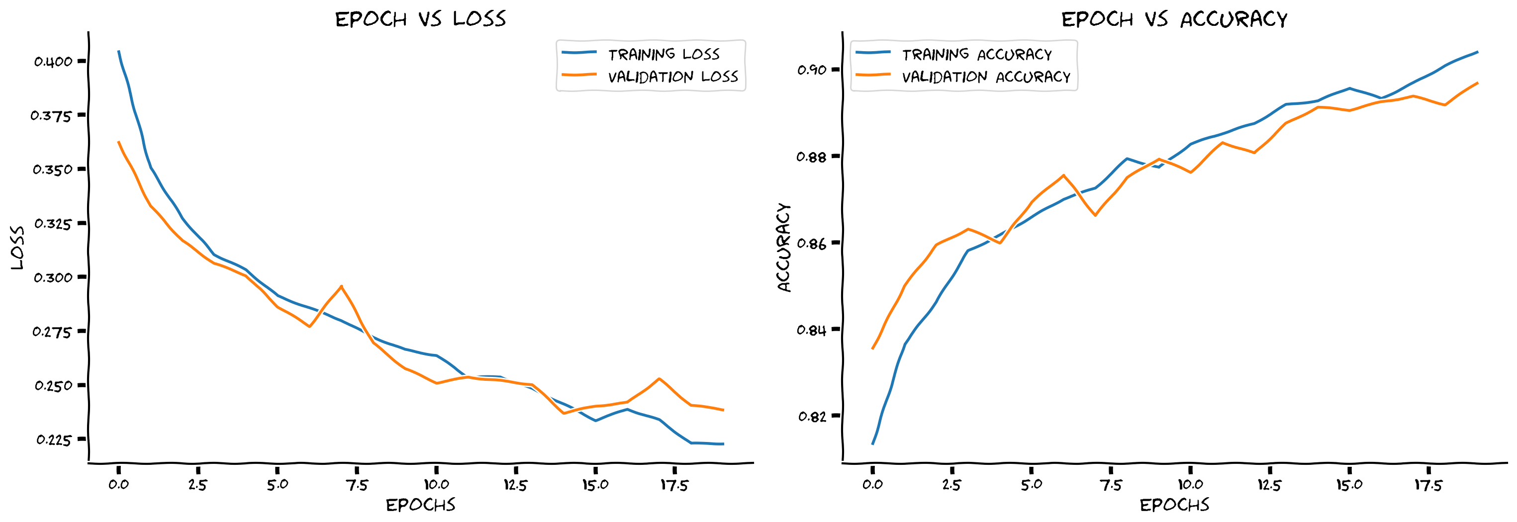
# @title Submit your feedback
content_review(f"{feedback_prefix}_How_much_augmentation_help_Bonus_Exercise")
考えてみよう!ボーナス 2.2: データ拡張
ドロップアウトのみの場合と比べてトレーニング精度はさらに下がりましたか?モデルはまだ過学習していますか?
素晴らしい!このセクションでは、おそらく初めてのCNNをトレーニングしました。正則化とデータ拡張を加えて、よく汎化するモデルを作りました。すべての要素が徐々に繋がってきています!
# @title Submit your feedback
content_review(f"{feedback_prefix}_Data_Augmentation_Bonus_Discussion")