チュートリアル 1: 正則化手法 パート1

第2週、第1日目: 正則化

Neuromatch Academyによる

コンテンツ作成者: ラヴィ・テジャ・コンキマラ、モヒトラジュ・リンガン・クマライアン、ケビン・マチャド・ガンボア、ケルソン・シリング-スクリボ、ライル・アングラー

コンテンツレビュアー: ピユシュ・チャウハン、バイ・スイウェイ、ケルソン・シリング-スクリボ

コンテンツ編集者: ロベルト・グイドッティ、スピロス・チャヴリス

制作編集者: サイード・サレヒ、ガガナ・B、スピロス・チャヴリス

チュートリアルの目的

1. 大規模な人工ニューラルネットワーク（ANN）は適応的基底関数により効率的な普遍近似器である
2. ANNは一部を記憶するが、良く一般化する
3. 過剰パラメータ化モデルの縮小としての正則化：早期終了

# @title Tutorial slides
from IPython.display import IFrame
link_id = "mf79a"
print(f"If you want to download the slides: https://osf.io/download/{link_id}/")
IFrame(src=f"https://mfr.ca-1.osf.io/render?url=https://osf.io/{link_id}/?direct%26mode=render%26action=download%26mode=render", width=854, height=480)

セットアップ

本日のコードの一部は実行に最大1時間かかる場合があります。そのため、コードは「非表示」にし、結果の出力のみを示しています。

# @title Install dependencies

# @markdown **WARNING**: There may be *errors* and/or *warnings* reported during the installation. However, they should be ignored.

# @title Install and import feedback gadget


from vibecheck import DatatopsContentReviewContainer
def content_review(notebook_section: str):
    return DatatopsContentReviewContainer(
        "",  # No text prompt
        notebook_section,
        {
            "url": "https://pmyvdlilci.execute-api.us-east-1.amazonaws.com/klab",
            "name": "neuromatch_dl",
            "user_key": "f379rz8y",
        },
    ).render()


feedback_prefix = "W2D1_T1"

# Imports
import time
import copy
import torch
import pathlib

import numpy as np
import torch.nn as nn
import torch.optim as optim
import torch.nn.functional as F
import matplotlib.pyplot as plt
import matplotlib.animation as animation

from tqdm.auto import tqdm
from IPython.display import HTML
from torchvision import transforms
from torchvision.datasets import ImageFolder

# @title Figure Settings
import logging
logging.getLogger('matplotlib.font_manager').disabled = True

import ipywidgets as widgets
%matplotlib inline
%config InlineBackend.figure_format = 'retina'
plt.style.use("https://raw.githubusercontent.com/NeuromatchAcademy/content-creation/main/nma.mplstyle")

# @title Loading Animal Faces data
import requests, os
from zipfile import ZipFile

print("Start downloading and unzipping `AnimalFaces` dataset...")
name = 'afhq'
fname = f"{name}.zip"
url = f"https://osf.io/kgfvj/download"

if not os.path.exists(fname):
  r = requests.get(url, allow_redirects=True)
  with open(fname, 'wb') as fh:
    fh.write(r.content)

  if os.path.exists(fname):
    with ZipFile(fname, 'r') as zfile:
      zfile.extractall(f".")
      os.remove(fname)

print("Download completed.")

# @title Loading Animal Faces Randomized data

print("Start downloading and unzipping `Randomized AnimalFaces` dataset...")

names = ['afhq_random_32x32', 'afhq_10_32x32']
urls = ["https://osf.io/9sj7p/download",
        "https://osf.io/wvgkq/download"]


for i, name in enumerate(names):
  url = urls[i]
  fname = f"{name}.zip"

  if not os.path.exists(fname):
    r = requests.get(url, allow_redirects=True)
    with open(fname, 'wb') as fh:
      fh.write(r.content)

    if os.path.exists(fname):
      with ZipFile(fname, 'r') as zfile:
        zfile.extractall(f".")
        os.remove(fname)

print("Download completed.")

# @title Plotting functions
def imshow(img):
  """
  Display unnormalized image

  Args:
    img: np.ndarray
      Datapoint to visualize

  Returns:
    Nothing
  """
  img = img / 2 + 0.5     # Unnormalize
  npimg = img.numpy()
  plt.imshow(np.transpose(npimg, (1, 2, 0)))
  plt.axis(False)
  plt.show()


def plot_weights(norm, labels, ws,
                 title='Weight Size Measurement'):
  """
  Plot of weight size measurement [norm value vs layer]

  Args:
    norm: float
      Norm values
    labels: list
      Targets
    ws: list
      Weights
    title: string
      Title of plot

  Returns:
    Nothing
  """
  plt.figure(figsize=[8, 6])
  plt.title(title)
  plt.ylabel('Frobenius Norm Value')
  plt.xlabel('Model Layers')
  plt.bar(labels, ws)
  plt.axhline(y=norm,
              linewidth=1,
              color='r',
              ls='--',
              label='Total Model F-Norm')
  plt.legend()
  plt.show()


def early_stop_plot(train_acc_earlystop,
                    val_acc_earlystop, best_epoch):
  """
  Plot of early stopping

  Args:
    train_acc_earlystop: np.ndarray
      Training accuracy log until early stop point
    val_acc_earlystop: np.ndarray
      Val accuracy log until early stop point
    best_epoch: int
      Epoch at which early stopping occurs

  Returns:
    Nothing
  """
  plt.figure(figsize=(8, 6))
  plt.plot(val_acc_earlystop,label='Val - Early',c='red',ls = 'dashed')
  plt.plot(train_acc_earlystop,label='Train - Early',c='red',ls = 'solid')
  plt.axvline(x=best_epoch, c='green', ls='dashed',
              label='Epoch for Max Val Accuracy')
  plt.title('Early Stopping')
  plt.ylabel('Accuracy (%)')
  plt.xlabel('Epoch')
  plt.legend()
  plt.show()

# @title Set random seed

# @markdown Executing `set_seed(seed=seed)` you are setting the seed

# For DL its critical to set the random seed so that students can have a
# baseline to compare their results to expected results.
# Read more here: https://pytorch.org/docs/stable/notes/randomness.html

# Call `set_seed` function in the exercises to ensure reproducibility.
import random
import torch

def set_seed(seed=None, seed_torch=True):
  """
  Function that controls randomness. NumPy and random modules must be imported.

  Args:
    seed : Integer
      A non-negative integer that defines the random state. Default is `None`.
    seed_torch : Boolean
      If `True` sets the random seed for pytorch tensors, so pytorch module
      must be imported. Default is `True`.

  Returns:
    Nothing.
  """
  if seed is None:
    seed = np.random.choice(2 ** 32)
  random.seed(seed)
  np.random.seed(seed)
  if seed_torch:
    torch.manual_seed(seed)
    torch.cuda.manual_seed_all(seed)
    torch.cuda.manual_seed(seed)
    torch.backends.cudnn.benchmark = False
    torch.backends.cudnn.deterministic = True

  print(f'Random seed {seed} has been set.')


# In case that `DataLoader` is used
def seed_worker(worker_id):
  """
  DataLoader will reseed workers following randomness in
  multi-process data loading algorithm.

  Args:
    worker_id: integer
      ID of subprocess to seed. 0 means that
      the data will be loaded in the main process
      Refer: https://pytorch.org/docs/stable/data.html#data-loading-randomness for more details

  Returns:
    Nothing
  """
  worker_seed = torch.initial_seed() % 2**32
  np.random.seed(worker_seed)
  random.seed(worker_seed)

# @title Set device (GPU or CPU). Execute `set_device()`
# especially if torch modules used.

# Inform the user if the notebook uses GPU or CPU.

def set_device():
  """
  Set the device. CUDA if available, CPU otherwise

  Args:
    None

  Returns:
    Nothing
  """
  device = "cuda" if torch.cuda.is_available() else "cpu"
  if device != "cuda":
    print("WARNING: For this notebook to perform best, "
        "if possible, in the menu under `Runtime` -> "
        "`Change runtime type.`  select `GPU` ")
  else:
    print("GPU is enabled in this notebook.")

  return device

SEED = 2021
set_seed(seed=SEED)
DEVICE = set_device()

セクション0: 便利な関数の定義

本チュートリアルを始めるにあたり、今日頻繁に使う関数、例えば AnimalNet、train、test、main を定義しましょう。

class AnimalNet(nn.Module):
  """
  Network Class - Animal Faces
  """

  def __init__(self):
    """
    Initialize parameters of AnimalNet

    Args:
      None

    Returns:
      Nothing
    """
    super(AnimalNet, self).__init__()
    self.fc1 = nn.Linear(3 * 32 * 32, 128)
    self.fc2 = nn.Linear(128, 32)
    self.fc3 = nn.Linear(32, 3)

  def forward(self, x):
    """
    Forward Pass of AnimalNet

    Args:
      x: torch.tensor
        Input features

    Returns:
      output: torch.tensor
        Outputs/Predictions
    """
    x = x.view(x.shape[0],-1)
    x = F.relu(self.fc1(x))
    x = F.relu(self.fc2(x))
    x = self.fc3(x)
    output = F.log_softmax(x, dim=1)
    return output

train関数は現在のモデルとtrain_loader、損失関数を受け取り、データセット全体を1回通してパラメータを更新します。test関数は各エポック後の現在のモデルを受け取り、テストデータセットの精度を計算します。

def train(args, model, train_loader, optimizer,
          reg_function1=None, reg_function2=None, criterion=F.nll_loss):
  """
  Trains the current input model using the data
  from Train_loader and Updates parameters for a single pass

  Args:
    args: dictionary
      Dictionary with epochs: 200, lr: 5e-3, momentum: 0.9, device: DEVICE
    model: nn.module
      Neural network instance
    train_loader: torch.loader
      Input dataset
    optimizer: function
      Optimizer
    reg_function1: function
      Regularisation function [default: None]
    reg_function2: function
      Regularisation function [default: None]
    criterion: function
      Specifies loss function [default: nll_loss]

  Returns:
    model: nn.module
      Neural network instance post training
  """
  device = args['device']
  model.train()
  for batch_idx, (data, target) in enumerate(train_loader):
    data, target = data.to(device), target.to(device)
    optimizer.zero_grad()
    output = model(data)
    if reg_function1 is None:
      loss = criterion(output, target)
    elif reg_function2 is None:
      loss = criterion(output, target)+args['lambda']*reg_function1(model)
    else:
      loss = criterion(output, target) + args['lambda1']*reg_function1(model) + args['lambda2']*reg_function2(model)
    loss.backward()
    optimizer.step()

  return model


def test(model, test_loader, criterion=F.nll_loss, device='cpu'):
  """
  Tests the current model

  Args:
    model: nn.module
      Neural network instance
    device: string
      GPU/CUDA if available, CPU otherwise
    test_loader: torch.loader
      Test dataset
    criterion: function
      Specifies loss function [default: nll_loss]

  Returns:
    test_loss: float
      Test loss
  """
  model.eval()
  test_loss = 0
  correct = 0
  with torch.no_grad():
    for data, target in test_loader:
      data, target = data.to(device), target.to(device)
      output = model(data)
      test_loss += criterion(output, target, reduction='sum').item()  # Sum up batch loss
      pred = output.argmax(dim=1, keepdim=True)  # Get the index of the max log-probability
      correct += pred.eq(target.view_as(pred)).sum().item()

  test_loss /= len(test_loader.dataset)
  return 100. * correct / len(test_loader.dataset)


def main(args, model, train_loader, val_loader,
         reg_function1=None, reg_function2=None):
  """
  Trains the model with train_loader and
  tests the learned model using val_loader

  Args:
    args: dictionary
      Dictionary with epochs: 200, lr: 5e-3, momentum: 0.9, device: DEVICE
    model: nn.module
      Neural network instance
    train_loader: torch.loader
      Train dataset
    val_loader: torch.loader
      Validation set
    reg_function1: function
      Regularisation function [default: None]
    reg_function2: function
      Regularisation function [default: None]

  Returns:
    val_acc_list: list
      Log of validation accuracy
    train_acc_list: list
      Log of training accuracy
    param_norm_list: list
      Log of frobenius norm
    trained_model: nn.module
      Trained model/model post training
  """

  device = args['device']

  model = model.to(device)
  optimizer = optim.SGD(model.parameters(), lr=args['lr'],
                        momentum=args['momentum'])

  val_acc_list, train_acc_list,param_norm_list = [], [], []
  for epoch in tqdm(range(args['epochs'])):
    trained_model = train(args, model, train_loader, optimizer,
                          reg_function1=reg_function1,
                          reg_function2=reg_function2)
    train_acc = test(trained_model, train_loader, device=device)
    val_acc = test(trained_model, val_loader, device=device)
    param_norm = calculate_frobenius_norm(trained_model)
    train_acc_list.append(train_acc)
    val_acc_list.append(val_acc)
    param_norm_list.append(param_norm)

  return val_acc_list, train_acc_list, param_norm_list, trained_model

セクション1: 正則化は縮小である

所要時間の目安：約20分

# @title Video 1: Introduction to Regularization
from ipywidgets import widgets
from IPython.display import YouTubeVideo
from IPython.display import IFrame
from IPython.display import display


class PlayVideo(IFrame):
  def __init__(self, id, source, page=1, width=400, height=300, **kwargs):
    self.id = id
    if source == 'Bilibili':
      src = f'https://player.bilibili.com/player.html?bvid={id}&page={page}'
    elif source == 'Osf':
      src = f'https://mfr.ca-1.osf.io/render?url=https://osf.io/download/{id}/?direct%26mode=render'
    super(PlayVideo, self).__init__(src, width, height, **kwargs)


def display_videos(video_ids, W=400, H=300, fs=1):
  tab_contents = []
  for i, video_id in enumerate(video_ids):
    out = widgets.Output()
    with out:
      if video_ids[i][0] == 'Youtube':
        video = YouTubeVideo(id=video_ids[i][1], width=W,
                             height=H, fs=fs, rel=0)
        print(f'Video available at https://youtube.com/watch?v={video.id}')
      else:
        video = PlayVideo(id=video_ids[i][1], source=video_ids[i][0], width=W,
                          height=H, fs=fs, autoplay=False)
        if video_ids[i][0] == 'Bilibili':
          print(f'Video available at https://www.bilibili.com/video/{video.id}')
        elif video_ids[i][0] == 'Osf':
          print(f'Video available at https://osf.io/{video.id}')
      display(video)
    tab_contents.append(out)
  return tab_contents


video_ids = [('Youtube', 'jhQAnIHTR6A'), ('Bilibili', 'BV1mo4y1X76E')]
tab_contents = display_videos(video_ids, W=854, H=480)
tabs = widgets.Tab()
tabs.children = tab_contents
for i in range(len(tab_contents)):
  tabs.set_title(i, video_ids[i][0])
display(tabs)

# @title Submit your feedback
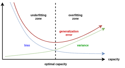
content_review(f"{feedback_prefix}_Introduction_to_Regularization_Video")

ニューラルネットの重要な考え方は、「複雑すぎる」モデルを使うことです。これはデータのノイズまでフィットできるほど複雑です。そこでモデルを「正則化」して、複雑すぎず十分に複雑な状態に調整します。モデルが複雑であるほど訓練データに良く適合しますが、複雑すぎると一般化性能が低下します。つまり訓練データを記憶してしまい、将来のテストデータに対しては精度が落ちます。

# @title Video 2: Regularization as Shrinkage
from ipywidgets import widgets
from IPython.display import YouTubeVideo
from IPython.display import IFrame
from IPython.display import display


class PlayVideo(IFrame):
  def __init__(self, id, source, page=1, width=400, height=300, **kwargs):
    self.id = id
    if source == 'Bilibili':
      src = f'https://player.bilibili.com/player.html?bvid={id}&page={page}'
    elif source == 'Osf':
      src = f'https://mfr.ca-1.osf.io/render?url=https://osf.io/download/{id}/?direct%26mode=render'
    super(PlayVideo, self).__init__(src, width, height, **kwargs)


def display_videos(video_ids, W=400, H=300, fs=1):
  tab_contents = []
  for i, video_id in enumerate(video_ids):
    out = widgets.Output()
    with out:
      if video_ids[i][0] == 'Youtube':
        video = YouTubeVideo(id=video_ids[i][1], width=W,
                             height=H, fs=fs, rel=0)
        print(f'Video available at https://youtube.com/watch?v={video.id}')
      else:
        video = PlayVideo(id=video_ids[i][1], source=video_ids[i][0], width=W,
                          height=H, fs=fs, autoplay=False)
        if video_ids[i][0] == 'Bilibili':
          print(f'Video available at https://www.bilibili.com/video/{video.id}')
        elif video_ids[i][0] == 'Osf':
          print(f'Video available at https://osf.io/{video.id}')
      display(video)
    tab_contents.append(out)
  return tab_contents


video_ids = [('Youtube', 'mhVbJ74upnQ'), ('Bilibili', 'BV1YL411H7Dv')]
tab_contents = display_videos(video_ids, W=854, H=480)
tabs = widgets.Tab()
tabs.children = tab_contents
for i in range(len(tab_contents)):
  tabs.set_title(i, video_ids[i][0])
display(tabs)

# @title Submit your feedback
content_review(f"{feedback_prefix}_Regularization_as_Shrinkage_Video")

正則化を考える一つの方法は、モデル全体の重みの大きさで考えることです。大きな重みを持つモデルはデータに完璧にフィットできますが、小さな重みのモデルは訓練セットでの性能は劣る傾向にあるものの、驚くほどテストセットで良い結果を出すことがあります。重みが小さすぎるとモデルが過小適合してしまう問題もあります。

このチュートリアルでは、モデル内のすべてのテンソルのフロベニウスノルムの和を「モデルの大きさ」の指標として使います。

コーディング演習1: フロベニウスノルム

始める前に、フロベニウスノルム（時にユークリッドノルムとも呼ばれる）を定義しましょう。$m×n$行列$A$のフロベニウスノルムは、その要素の絶対値の二乗和の平方根として定義されます。

これは単に行列の大きさを測る指標であり、ベクトルの大きさに相当します。

ヒント: model.parameters() または $model.named_parameters()$ 関数を使いましょう

def calculate_frobenius_norm(model):
  """
  Function to calculate frobenius norm

  Args:
    model: nn.module
      Neural network instance

  Returns:
    norm: float
      Frobenius norm
  """
  ####################################################################
  # Fill in all missing code below (...),
  # then remove or comment the line below to test your function
  raise NotImplementedError("Define `calculate_frobenius_norm` function")
  ####################################################################
  norm = 0.0
  # Sum the square of all parameters
  for param in model.parameters():
    norm += ...

  # Take a square root of the sum of squares of all the parameters
  norm = ...
  return norm



# Seed added for reproducibility
set_seed(seed=SEED)

## uncomment below to test your code
# net = nn.Linear(10, 1)
# print(f'Frobenius norm of Single Linear Layer: {calculate_frobenius_norm(net)}')

ランダムシード2021が設定されました。
単一線形層のフロベニウスノルム: 0.6572162508964539

解答を見る$

# @title Submit your feedback
content_review(f"{feedback_prefix}_Forbenius_norm_Exercise")

モデル全体の重みの大きさを計算するだけでなく、各層ごとの重みの大きさも求めることができます。そのために、calculate_frobenius_norm関数を以下のように修正します。

どのように動作するか見てみましょう！

def calculate_frobenius_norm(model):
  """
  Calculate Frobenius Norm per Layer

  Args:
    model: nn.module
      Neural network instance

  Returns:
    norm: float
      Norm value
    labels: list
      Targets
    ws: list
      Weights
  """

  # Initialization of variables
  norm, ws, labels = 0.0, [], []

  # Sum all the parameters
  for name, parameters in model.named_parameters():
    p = torch.sum(parameters**2)
    norm += p

    ws.append((p**0.5).cpu().detach().numpy())
    labels.append(name)

  # Take a square root of the sum of squares of all the parameters
  norm = (norm**0.5).cpu().detach().numpy()

  return norm, ws, labels


set_seed(SEED)
net = nn.Linear(10,1)
norm, ws, labels = calculate_frobenius_norm(net)
print(f'Frobenius norm of Single Linear Layer: {norm:.4f}')
# Plots the weights
plot_weights(norm, labels, ws)

最後の関数 calculate_frobenius_norm を使うことで、ANNモデル全体の各層ごとのフロベニウスノルムを取得し、plot_weights関数で可視化できます。

set_seed(seed=SEED)

# Creates a new model
model = AnimalNet()

# Calculates the forbenius norm per layer
norm, ws, labels = calculate_frobenius_norm(model)
print(f'Frobenius norm of Models weights: {norm:.4f}')

# Plots the weights
plot_weights(norm, labels, ws)

セクション2: 過学習

所要時間の目安：約15分

# @title Video 3: Overparameterization and Overfitting
from ipywidgets import widgets
from IPython.display import YouTubeVideo
from IPython.display import IFrame
from IPython.display import display


class PlayVideo(IFrame):
  def __init__(self, id, source, page=1, width=400, height=300, **kwargs):
    self.id = id
    if source == 'Bilibili':
      src = f'https://player.bilibili.com/player.html?bvid={id}&page={page}'
    elif source == 'Osf':
      src = f'https://mfr.ca-1.osf.io/render?url=https://osf.io/download/{id}/?direct%26mode=render'
    super(PlayVideo, self).__init__(src, width, height, **kwargs)


def display_videos(video_ids, W=400, H=300, fs=1):
  tab_contents = []
  for i, video_id in enumerate(video_ids):
    out = widgets.Output()
    with out:
      if video_ids[i][0] == 'Youtube':
        video = YouTubeVideo(id=video_ids[i][1], width=W,
                             height=H, fs=fs, rel=0)
        print(f'Video available at https://youtube.com/watch?v={video.id}')
      else:
        video = PlayVideo(id=video_ids[i][1], source=video_ids[i][0], width=W,
                          height=H, fs=fs, autoplay=False)
        if video_ids[i][0] == 'Bilibili':
          print(f'Video available at https://www.bilibili.com/video/{video.id}')
        elif video_ids[i][0] == 'Osf':
          print(f'Video available at https://osf.io/{video.id}')
      display(video)
    tab_contents.append(out)
  return tab_contents


video_ids = [('Youtube', '-HJ_9HxY38g'), ('Bilibili', 'BV1NX4y1A73i')]
tab_contents = display_videos(video_ids, W=854, H=480)
tabs = widgets.Tab()
tabs.children = tab_contents
for i in range(len(tab_contents)):
  tabs.set_title(i, video_ids[i][0])
display(tabs)

# @title Submit your feedback
content_review(f"{feedback_prefix}_Overparameterization_and_Overfitting_Video")

セクション2.1: 過学習の可視化

ニューラルネットの過学習を説明するために、合成データセットを作成しましょう。

set_seed(seed=SEED)

# Creating train data
# Input
X = torch.rand((10, 1))
# Output
Y = 2*X + 2*torch.empty((X.shape[0], 1)).normal_(mean=0, std=1)  # Adding small error in the data

# Visualizing train data
plt.figure(figsize=(8, 6))
plt.scatter(X.numpy(),Y.numpy())
plt.xlabel('input (x)')
plt.ylabel('output(y)')
plt.title('toy dataset')
plt.show()

# Creating test dataset
X_test = torch.linspace(0, 1, 40)
X_test = X_test.reshape((40, 1, 1))

先ほど作成したデータセットにフィットできる過剰パラメータ化されたニューラルネットを作成し、訓練します。

まずはモデルのアーキテクチャを構築しましょう。

class Net(nn.Module):
  """
  Network Class - 2D with following structure
  nn.Linear(1, 300) + leaky_relu(self.fc1(x)) # First fully connected layer
  nn.Linear(300, 500) + leaky_relu(self.fc2(x)) # Second fully connected layer
  nn.Linear(500, 1) # Final fully connected layer
  """

  def __init__(self):
    """
    Initialize parameters of Net

    Args:
      None

    Returns:
      Nothing
    """
    super(Net, self).__init__()

    self.fc1 = nn.Linear(1, 300)
    self.fc2 = nn.Linear(300, 500)
    self.fc3 = nn.Linear(500, 1)

  def forward(self, x):
    """
    Forward pass of Net

    Args:
      x: torch.tensor
        Input features

    Returns:
      x: torch.tensor
        Output/Predictions
    """
    x = F.leaky_relu(self.fc1(x))
    x = F.leaky_relu(self.fc2(x))
    output = self.fc3(x)
    return output

次に、モデルの訓練に必要な各種パラメータを定義します。

set_seed(seed=SEED)

# Train the network on toy dataset
model = Net()

criterion = nn.MSELoss()
optimizer = optim.Adam(model.parameters(), lr=1e-4)

iters = 0
# Calculates frobenius before training
normi, wsi, label = calculate_frobenius_norm(model)

これでモデルの訓練を開始できます。

set_seed(seed=SEED)

# Initializing variables
# Losses
train_loss = []
test_loss = []

# Model norm
model_norm = []

# Initializing variables to store weights
norm_per_layer = []

max_epochs = 10000

running_predictions = np.empty((40, int(max_epochs / 500 + 1)))

for epoch in tqdm(range(max_epochs)):
  # Frobenius norm per epoch
  norm, pl, layer_names = calculate_frobenius_norm(model)

  # Training
  model_norm.append(norm)
  norm_per_layer.append(pl)
  model.train()
  optimizer.zero_grad()
  predictions = model(X)
  loss = criterion(predictions, Y)
  loss.backward()
  optimizer.step()

  train_loss.append(loss.data)
  model.eval()
  Y_test = model(X_test)
  loss = criterion(Y_test, 2*X_test)
  test_loss.append(loss.data)

  if (epoch % 500 == 0 or epoch == max_epochs - 1):
    running_predictions[:, iters] = Y_test[:, 0, 0].detach().numpy()
    iters += 1

訓練が終わったので、訓練過程でモデルがどのように変化したか見てみましょう。

# @title Animation (Run Me!)

set_seed(seed=SEED)
# Create a figure and axes
fig = plt.figure(figsize=(14, 5))
ax1 = plt.subplot(121)
ax2 = plt.subplot(122)
# Organizing subplots
plot1, = ax1.plot([],[])
plot2 = ax2.bar([], [])


def frame(i):
  """
  Load animation frame

  Args:
    i: int
      Epoch number

  Returns:
    plot1: function
      Subplot of test-data vs running predictions
    plot2: function
      Subplot of test-data vs running predictions
  """
  ax1.clear()
  title1 = ax1.set_title('')
  ax1.set_xlabel("Input(x)")
  ax1.set_ylabel("Output(y)")

  ax2.clear()
  ax2.set_xlabel('Layer names')
  ax2.set_ylabel('Frobenius norm')
  title2 = ax2.set_title('Weight Measurement: Forbenius Norm')

  ax1.scatter(X.numpy(),Y.numpy())
  plot1 = ax1.plot(X_test[:,0,:].detach().numpy(),
                   running_predictions[:,i])
  title1.set_text(f'Epochs: {i * 500}')
  plot2 = ax2.bar(label, norm_per_layer[i*500])
  plt.axhline(y=model_norm[i*500], linewidth=1,
              color='r', ls='--',
              label=f'Norm: {model_norm[i*500]:.2f}')
  plt.legend()

  return plot1, plot2


anim = animation.FuncAnimation(fig, frame, frames=range(20),
                               blit=False, repeat=False,
                               repeat_delay=10000)
html_anim = HTML(anim.to_html5_video())
plt.close()

import IPython
IPython.display.display(html_anim)

# @title Plot the train and test losses
plt.figure(figsize=(8, 6))
plt.plot(train_loss,label='train_loss')
plt.plot(test_loss,label='test_loss')
plt.ylabel('loss')
plt.xlabel('epochs')
plt.title('loss vs epoch')
plt.legend()
plt.show()

考えてみよう！2.1: 損失の解釈

上の訓練とテストのグラフについて、以下を話し合ってみてください：

• 訓練損失とテスト損失の傾向はどうなっていますか？（損失の最小値はどこにありますか？）
• これが私たちの訓練したモデルについて何を示していますか？

解答を見る$

# @title Submit your feedback
content_review(f"{feedback_prefix}_Interpreting_losses_Discussion")

次に、訓練中のモデルのフロベニウスノルムを可視化しましょう。エポックが進むにつれて重みの値が増加しているのが見えるはずです。

# @markdown Frobenious norm of the model
plt.figure(figsize=(8, 6))
plt.plot(model_norm)
plt.ylabel('Norm of the model')
plt.xlabel('Epochs')
plt.title('Frobenious norm of the model')
plt.show()

最後に、トレーニング前後のモデルの各層ごとのフロベニウスノルムを比較できます。

# @markdown Frobenius norm per layer before and after training
normf, wsf, label = calculate_frobenius_norm(model)

plot_weights(float(normi), label, wsi,
             title='Weight Size Before Training')
plot_weights(float(normf), label, wsf,
             title='Weight Size After Training')

セクション 2.2: テストデータセットでの過学習

原則として、すべてのハイパーパラメータを選択するまでテストセットには触れてはいけません。もしモデル選択の過程でテストデータを使用すると、テストデータに過学習してしまうリスクがあり、それは非常に深刻な問題になります。トレーニングデータに過学習した場合は、テストデータを使った評価が常にあり、モデルの正当性を保てます。しかし、テストデータに過学習してしまったら、どうやってそれを知ることができるでしょうか？

また別の種類の過学習もあります。ある画像や投稿、医療記録のセットに対して「正直な」フィッティングを行っても、それが他の画像や投稿、医療記録に一般化しない場合です。

バリデーションデータセット

この問題に対処する一般的な方法は、データを3つに分割し、ハイパーパラメータの調整にバリデーションデータセット（またはバリデーションセット）を使うことです。理想的には、テストデータには一度だけ触れて、最良のモデルを評価したり、少数のモデル同士を比較したりします。実際のテストデータは一度使っただけで捨てられることはほとんどありません。

セクション 3: 記憶

所要時間の目安: 約20分

十分に大きなネットワークと十分なトレーニングがあれば、ニューラルネットワークは各トレーニング例を記憶することでほぼ100%のトレーニング精度を達成できます。しかし、これは新しいデータに対してモデルが失敗することを意味するため望ましくありません。

このセクションでは、3つのMLPをトレーニングします。対象はそれぞれ：

1. 動物の顔データセット
2. 完全にノイズのあるデータセット（すべてのラベルをランダムにシャッフル）
3. 部分的にノイズのあるデータセット（15%のラベルをランダムにシャッフル）

さて、十分な時間トレーニングし強力なネットワークを使った場合、これらのモデルのトレーニング精度とテスト精度はどうなるか、数分考えてみてください。

まず、3つのデータセットすべてに必要なデータローダーを作成しましょう。データの分割方法に注目してください。データセットの一部でトレーニングするのは、トレーニングが速くなり、過学習がより明確に見えるためです。

# Dataloaders for the Dataset
batch_size = 128
classes = ('cat', 'dog', 'wild')

# Defining number of examples for train, val test
len_train, len_val, len_test = 100, 100, 14430

train_transform = transforms.Compose([
     transforms.ToTensor(),
     transforms.Normalize((0.5, 0.5, 0.5), (0.5, 0.5, 0.5))
     ])
data_path = pathlib.Path('.')/'afhq'  # Using pathlib to be compatible with all OS's
img_dataset = ImageFolder(data_path/'train', transform=train_transform)

# Dataloaders for the Original Dataset

# For reproducibility
g_seed = torch.Generator()
g_seed.manual_seed(SEED)

img_train_data, img_val_data,_ = torch.utils.data.random_split(img_dataset,
                                                               [len_train,
                                                                len_val,
                                                                len_test])

# Creating train_loader and Val_loader
train_loader = torch.utils.data.DataLoader(img_train_data,
                                           batch_size=batch_size,
                                           num_workers=2,
                                           worker_init_fn=seed_worker,
                                           generator=g_seed)

val_loader = torch.utils.data.DataLoader(img_val_data,
                                         batch_size=1000,
                                         num_workers=2,
                                         worker_init_fn=seed_worker,
                                         generator=g_seed)

# Dataloaders for the Random Dataset

# For reproducibility
g_seed = torch.Generator()
g_seed.manual_seed(SEED + 1)

# Splitting randomized data into training and validation data
data_path = pathlib.Path('.')/'afhq_random_32x32/afhq_random' # Using pathlib to be compatible with all OS's
img_dataset = ImageFolder(data_path/'train', transform=train_transform)
random_img_train_data, random_img_val_data,_ = torch.utils.data.random_split(img_dataset, [len_train, len_val, len_test])

# Randomized train and validation dataloader
rand_train_loader = torch.utils.data.DataLoader(random_img_train_data,
                                                batch_size=batch_size,
                                                num_workers=2,
                                                worker_init_fn=seed_worker,
                                                generator=g_seed)

rand_val_loader = torch.utils.data.DataLoader(random_img_val_data,
                                              batch_size=1000,
                                              num_workers=2,
                                              worker_init_fn=seed_worker,
                                              generator=g_seed)

# Dataloaders for the Partially Random Dataset

# For reproducibility
g_seed = torch.Generator()
g_seed.manual_seed(SEED + 1)

# Splitting data between training and validation dataset for partially randomized data
data_path = pathlib.Path('.')/'afhq_10_32x32/afhq_10' # Using pathlib to be compatible with all OS's
img_dataset = ImageFolder(data_path/'train', transform=train_transform)
partially_random_train_data, partially_random_val_data,_ = torch.utils.data.random_split(img_dataset, [len_train, len_val, len_test])

# Training and Validation loader for partially randomized data
partial_rand_train_loader = torch.utils.data.DataLoader(partially_random_train_data,
                                                        batch_size=batch_size,
                                                        num_workers=2,
                                                        worker_init_fn=seed_worker,
                                                        generator=g_seed)

partial_rand_val_loader = torch.utils.data.DataLoader(partially_random_val_data,
                                                      batch_size=1000,
                                                      num_workers=2,
                                                      worker_init_fn=seed_worker,
                                                      generator=g_seed)

次に、トレーニングデータセットのサイズに比べて多くのパラメータを持つモデルを定義し、これらのデータセットでトレーニングしましょう。

class BigAnimalNet(nn.Module):
  """
  Network Class - Animal Faces with following structure:
  nn.Linear(3*32*32, 124) + leaky_relu(self.fc1(x)) # First fully connected layer
  nn.Linear(124, 64) + leaky_relu(self.fc2(x)) # Second fully connected layer
  nn.Linear(64, 3) # Final fully connected layer
  """

  def __init__(self):
    """
    Initialize parameters for BigAnimalNet

    Args:
      None

    Returns:
      Nothing
    """
    super(BigAnimalNet, self).__init__()
    self.fc1 = nn.Linear(3*32*32, 124)
    self.fc2 = nn.Linear(124, 64)
    self.fc3 = nn.Linear(64, 3)

  def forward(self, x):
    """
    Forward pass of BigAnimalNet

    Args:
      x: torch.tensor
        Input features

    Returns:
      x: torch.tensor
        Output/Predictions
    """
    x = x.view(x.shape[0], -1)
    x = F.leaky_relu(self.fc1(x))
    x = F.leaky_relu(self.fc2(x))
    x = self.fc3(x)
    output = F.log_softmax(x, dim=1)
    return output

BigAnimalNet()をトレーニングする前に、再度フロベニウスノルムを計算します。

set_seed(seed=SEED)
normi, wsi, label = calculate_frobenius_norm(BigAnimalNet())

次に、BigAnimalNet()モデルをトレーニングします。

# Here we have 100 true train data.

# Set the arguments
args = {
    'epochs': 200,
    'lr': 5e-3,
    'momentum': 0.9,
    'device': DEVICE
}


# Initialize the network
set_seed(seed=SEED)
model = BigAnimalNet()

start_time = time.time()

# Train the network
val_acc_pure, train_acc_pure, _, model = main(args=args,
                                              model=model,
                                              train_loader=train_loader,
                                              val_loader=val_loader)
end_time = time.time()

print(f"Time to memorize the dataset: {end_time - start_time}")

# Train and Test accuracy plot
plt.figure(figsize=(8, 6))
plt.plot(val_acc_pure, label='Val Accuracy Pure', c='red', ls='dashed')
plt.plot(train_acc_pure, label='Train Accuracy Pure', c='red', ls='solid')
plt.axhline(y=max(val_acc_pure), c='green', ls='dashed',
            label='max Val accuracy pure')
plt.title('Memorization')
plt.ylabel('Accuracy (%)')
plt.xlabel('Epoch')
plt.legend()
plt.show()

# @markdown #### Frobenius norm for AnimalNet before and after training
normf, wsf, label = calculate_frobenius_norm(model)

plot_weights(float(normi), label, wsi, title='Weight Size Before Training')
plot_weights(float(normf), label, wsf, title='Weight Size After Training')

データビジュアライザー

ランダムラベルのデータでモデルをトレーニングする前に、データが本当にランダムであることを視覚化して確認しましょう。ここでは：

classes = ("cat", "dog", "wild")

.permute()メソッドを使います。plt.imshow()は入力がNumPy形式で、かつ$(P_x, P_y, 3)$の形式であることを期待しています。ここで$P_x$と$P_y$はそれぞれ$x$軸と$y$軸方向のピクセル数です。

def visualize_data(dataloader):
  """
  Helper function to visualize data

  Args:
    dataloader: torch.tensor
      Dataloader to visualize

  Returns:
    Nothing
  """

  for idx, (data, label) in enumerate(dataloader):
    plt.figure(idx)

    # Choose the datapoint you would like to visualize
    index = 22

    # Choose that datapoint using index and permute the dimensions
    # and bring the pixel values between [0, 1]
    data = data[index].permute(1, 2, 0) * \
           torch.tensor([0.5, 0.5, 0.5]) + \
           torch.tensor([0.5, 0.5, 0.5])

    # Convert the torch tensor into numpy
    data = data.numpy()

    plt.imshow(data)
    plt.axis(False)
    image_class = classes[label[index].item()]
    print(f'The image belongs to : {image_class}')

  plt.show()


# Call the function
visualize_data(rand_train_loader)

それでは、シャッフルされたデータでネットワークをトレーニングし、記憶しているかどうかを見てみましょう。

# Here we have 100 completely shuffled train data.

# Set the arguments
args = {
    'epochs': 200,
    'lr': 5e-3,
    'momentum': 0.9,
    'device': DEVICE
}

# Initialize the model
set_seed(seed=SEED)
model = BigAnimalNet()

# Train the model
val_acc_random, train_acc_random, _, model = main(args,
                                                  model,
                                                  rand_train_loader,
                                                  val_loader)

# Train and Test accuracy plot
plt.figure(figsize=(8, 6))
plt.plot(val_acc_pure,label='Val - Pure',c='red',ls = 'dashed')
plt.plot(train_acc_pure,label='Train - Pure',c='red',ls = 'solid')
plt.plot(val_acc_random,label='Val - Random',c='blue',ls = 'dashed')
plt.plot(train_acc_random,label='Train - Random',c='blue',ls = 'solid')

plt.title('Memorization')
plt.ylabel('Accuracy (%)')
plt.xlabel('Epoch')
plt.legend()
plt.show()

ANNがランダムにシャッフルされたラベルで100%のトレーニング精度を達成できたのは驚きではありませんか？これがトレーニング精度がモデルの性能を示す良い指標でない理由の一つです。

セクション 4: 早期停止

所要時間の目安: 約20分

# @title Video 4: Early Stopping
from ipywidgets import widgets
from IPython.display import YouTubeVideo
from IPython.display import IFrame
from IPython.display import display


class PlayVideo(IFrame):
  def __init__(self, id, source, page=1, width=400, height=300, **kwargs):
    self.id = id
    if source == 'Bilibili':
      src = f'https://player.bilibili.com/player.html?bvid={id}&page={page}'
    elif source == 'Osf':
      src = f'https://mfr.ca-1.osf.io/render?url=https://osf.io/download/{id}/?direct%26mode=render'
    super(PlayVideo, self).__init__(src, width, height, **kwargs)


def display_videos(video_ids, W=400, H=300, fs=1):
  tab_contents = []
  for i, video_id in enumerate(video_ids):
    out = widgets.Output()
    with out:
      if video_ids[i][0] == 'Youtube':
        video = YouTubeVideo(id=video_ids[i][1], width=W,
                             height=H, fs=fs, rel=0)
        print(f'Video available at https://youtube.com/watch?v={video.id}')
      else:
        video = PlayVideo(id=video_ids[i][1], source=video_ids[i][0], width=W,
                          height=H, fs=fs, autoplay=False)
        if video_ids[i][0] == 'Bilibili':
          print(f'Video available at https://www.bilibili.com/video/{video.id}')
        elif video_ids[i][0] == 'Osf':
          print(f'Video available at https://osf.io/{video.id}')
      display(video)
    tab_contents.append(out)
  return tab_contents


video_ids = [('Youtube', '72IG2bX5l30'), ('Bilibili', 'BV1cB4y1K777')]
tab_contents = display_videos(video_ids, W=854, H=480)
tabs = widgets.Tab()
tabs.children = tab_contents
for i in range(len(tab_contents)):
  tabs.set_title(i, video_ids[i][0])
display(tabs)

# @title Submit your feedback
content_review(f"{feedback_prefix}_Early_Stopping_Video")

バリデーション精度がモデルの過学習が始まる前にピークに達することがわかったので、トレーニングを早めに停止したいと思います。上のプロットからも、実データのトレーニング/テスト損失は非常に滑らかではなく、エポックの選択がバリデーション/テスト精度に重要な役割を果たすことが推測できるでしょう。

早期停止は、バリデーション精度が向上しなくなった時点でトレーニングを停止します。

コーディング演習 4: 早期停止

上記の説明に従って早期停止を含むようにメイン関数を再実装してください。その後、以下のコードを実行して実装を検証しましょう。

def early_stopping_main(args, model, train_loader, val_loader):
  """
  Function to simulate early stopping

  Args:
    args: dictionary
      Dictionary with epochs: 200, lr: 5e-3, momentum: 0.9, device: DEVICE
    model: nn.module
      Neural network instance
    train_loader: torch.loader
      Train dataset
    val_loader: torch.loader
      Validation set

  Returns:
    val_acc_list: list
      Val accuracy log until early stop point
    train_acc_list: list
      Training accuracy log until early stop point
    best_model: nn.module
      Model performing best with early stopping
    best_epoch: int
      Epoch at which early stopping occurs
  """

  ####################################################################
  # Fill in all missing code below (...),
  # then remove or comment the line below to test your function
  raise NotImplementedError("Complete the early_stopping_main function")
  ####################################################################
  device = args['device']
  model = model.to(device)
  optimizer = optim.SGD(model.parameters(),
                        lr=args['lr'],
                        momentum=args['momentum'])

  best_acc = 0.0
  best_epoch = 0

  # Number of successive epochs that you want to wait before stopping training process
  patience = 20

  # Keeps track of number of epochs during which the val_acc was less than best_acc
  wait = 0

  val_acc_list, train_acc_list = [], []
  for epoch in tqdm(range(args['epochs'])):

    # Train the model
    trained_model = ...

    # Calculate training accuracy
    train_acc = ...

    # Calculate validation accuracy
    val_acc = ...

    if (val_acc > best_acc):
      best_acc = val_acc
      best_epoch = epoch
      best_model = copy.deepcopy(trained_model)
      wait = 0
    else:
      wait += 1

    if (wait > patience):
      print(f'Early stopped on epoch: {epoch}')
      break

    train_acc_list.append(train_acc)
    val_acc_list.append(val_acc)

  return val_acc_list, train_acc_list, best_model, best_epoch



# Set the arguments
args = {
    'epochs': 200,
    'lr': 5e-4,
    'momentum': 0.99,
    'device': DEVICE
}

# Initialize the model
set_seed(seed=SEED)
model = AnimalNet()

## Uncomment to test
# val_acc_earlystop, train_acc_earlystop, best_model, best_epoch = early_stopping_main(args, model, train_loader, val_loader)
# print(f'Maximum Validation Accuracy is reached at epoch: {best_epoch:2d}')
# early_stop_plot(train_acc_earlystop, val_acc_earlystop, best_epoch)

解答を見る$

# @title Submit your feedback
content_review(f"{feedback_prefix}_Early_Stopping_Exercise")

考えてみよう！4: 早期停止

ポッド内で次のことについて議論してください：

• 早期停止はネットワークのトレーニングに悪影響を及ぼす可能性があると思いますか？

解答を見る$

# @title Submit your feedback
content_review(f"{feedback_prefix}_Early_Stopping_Discussion")

まとめ

このチュートリアルでは、シュリンケージとして説明される正則化手法を紹介しました。深層学習における最悪の落とし穴の一つである過学習について学び、最後にモデルの過学習を減らす方法として早期停止を学びました。

もし時間があれば、ランダム化されたラベルでトレーニングした場合のモデルの挙動について学べます。

ボーナス: ランダム化ラベルでのトレーニング

このパートでは、15%のラベルがノイズのある部分的にシャッフルされたデータセットでトレーニングしましょう。

# Here we have 15% partially shuffled train data.

# Set the arguments
args = {
    'epochs': 200,
    'lr': 5e-3,
    'momentum': 0.9,
    'device': DEVICE
}

# Intialize the model
set_seed(seed=SEED)
model = BigAnimalNet()

# Train the model
val_acc_shuffle, train_acc_shuffle, _, _, = main(args,
                                                 model,
                                                 partial_rand_train_loader,
                                                 val_loader)

# Train and test acc plot
plt.figure(figsize=(8, 6))
plt.plot(val_acc_shuffle, label='Val Accuracy shuffle', c='red', ls='dashed')
plt.plot(train_acc_shuffle, label='Train Accuracy shuffle', c='red', ls='solid')
plt.axhline(y=max(val_acc_shuffle), c='green', ls='dashed',
            label='Max Val Accuracy shuffle')
plt.title('Memorization')
plt.ylabel('Accuracy (%)')
plt.xlabel('Epoch')
plt.legend()
plt.show()

#@markdown #### Plotting them all together (Run Me!)
plt.figure(figsize=(8, 6))
plt.plot(val_acc_pure,label='Val - Pure',c='red',ls = 'dashed')
plt.plot(train_acc_pure,label='Train - Pure',c='red',ls = 'solid')
plt.plot(val_acc_random,label='Val - Random',c='blue',ls = 'dashed')
plt.plot(train_acc_random,label='Train - Random',c='blue',ls = 'solid')
plt.plot(val_acc_shuffle, label='Val - shuffle', c='y', ls='dashed')
plt.plot(train_acc_shuffle, label='Train - shuffle', c='y', ls='solid')

plt.title('Memorization')
plt.ylabel('Accuracy (%)')
plt.xlabel('Epoch')
plt.legend()
plt.show()

考えてみよう！ボーナス: 一般化しますか？

ニューラルネットワークがトレーニングデータを完全にフィット/記憶した場合：

• それは一般化できていると思いますか？
• なぜそう思うか、または思わないかの理由は何ですか？

解答を見る$

# @title Submit your feedback
content_review(f"{feedback_prefix}_Early_Stopping_Generalization_Bonus_Discussion")

また、わずかにシャッフルされたデータでトレーニングしたモデルが純粋なデータでトレーニングしたモデルよりわずかに良い結果を出すことがあるのは興味深い点です。データの一部をシャッフルすることは正則化の一形態であり、つまりトレーニングデータにノイズを加える多くの方法の一つです。