チュートリアル 2: 深いMLP

第1週、第3日目: 多層パーセプトロン

Neuromatch Academyによる

コンテンツ作成者: Arash Ash, Surya Ganguli

コンテンツレビュアー: Saeed Salehi, Felix Bartsch, Yu-Fang Yang, Melvin Selim Atay, Kelson Shilling-Scrivo

コンテンツ編集者: Gagana B, Kelson Shilling-Scrivo, Spiros Chavlis

制作編集者: Anoop Kulkarni, Kelson Shilling-Scrivo, Gagana B, Spiros Chavlis

チュートリアルの目的

このチュートリアルでは、MLPについてさらに深く掘り下げ、その数学的および実践的な側面を詳しく見ていきます。今日はMLPがなぜ以下のようになるのかを見ていきます:

深くも広くもできる
転送関数に依存する
初期化に敏感である

# @title Tutorial slides
from IPython.display import IFrame
link_id = "ed65b"
print(f"If you want to download the slides: https://osf.io/download/{link_id}/")
IFrame(src=f"https://mfr.ca-1.osf.io/render?url=https://osf.io/{link_id}/?direct%26mode=render%26action=download%26mode=render", width=854, height=480)

セットアップ

このノートブックはGPUを使用しません！

# @title Install and import feedback gadget


from vibecheck import DatatopsContentReviewContainer
def content_review(notebook_section: str):
    return DatatopsContentReviewContainer(
        "",  # No text prompt
        notebook_section,
        {
            "url": "https://pmyvdlilci.execute-api.us-east-1.amazonaws.com/klab",
            "name": "neuromatch_dl",
            "user_key": "f379rz8y",
        },
    ).render()


feedback_prefix = "W1D3_T2"

# Imports
import pathlib

import torch
import numpy as np
import matplotlib.pyplot as plt

import torch.nn as nn
import torch.optim as optim

from torchvision.utils import make_grid
import torchvision.transforms as transforms
from torchvision.datasets import ImageFolder
from torch.utils.data import DataLoader, TensorDataset

from tqdm.auto import tqdm
from IPython.display import display

# @title Figure Settings
import logging
logging.getLogger('matplotlib.font_manager').disabled = True

import ipywidgets as widgets  # Interactive display
%config InlineBackend.figure_format = 'retina'
plt.style.use("https://raw.githubusercontent.com/NeuromatchAcademy/content-creation/main/nma.mplstyle")
my_layout = widgets.Layout()

# @title Helper functions (MLP Tutorial 1 Codes)

# @markdown `Net(nn.Module)`

class Net(nn.Module):
  """
  Simulate MLP Network
  """

  def __init__(self, actv, input_feature_num, hidden_unit_nums, output_feature_num):
    """
    Initialize MLP Network parameters

    Args:
      actv: string
        Activation function
      input_feature_num: int
        Number of input features
      hidden_unit_nums: list
        Number of units per hidden layer. List of integers
      output_feature_num: int
        Number of output features

    Returns:
      Nothing
    """
    super(Net, self).__init__()
    self.input_feature_num = input_feature_num # Save the input size for reshapinng later
    self.mlp = nn.Sequential() # Initialize layers of MLP

    in_num = input_feature_num # Initialize the temporary input feature to each layer
    for i in range(len(hidden_unit_nums)): # Loop over layers and create each one
      out_num = hidden_unit_nums[i] # Assign the current layer hidden unit from list
      layer = nn.Linear(in_num, out_num) # Use nn.Linear to define the layer
      in_num = out_num # Assign next layer input using current layer output
      self.mlp.add_module(f"Linear_{i}", layer) # Append layer to the model with a name

      actv_layer = eval(f"nn.{actv}") # Assign activation function (eval allows us to instantiate object from string)
      self.mlp.add_module(f"Activation_{i}", actv_layer) # Append activation to the model with a name

    out_layer = nn.Linear(in_num, output_feature_num) # Create final layer
    self.mlp.add_module('Output_Linear', out_layer) # Append the final layer

  def forward(self, x):
    """
    Simulate forward pass of MLP Network

    Args:
      x: torch.tensor
        Input data

    Returns:
      logits: Instance of MLP
        Forward pass of MLP
    """
    # Reshape inputs to (batch_size, input_feature_num)
    # Just in case the input vector is not 2D, like an image!
    x = x.view(-1, self.input_feature_num)

    logits = self.mlp(x) # forward pass of MLP
    return logits


# @markdown `train_test_classification(net, criterion, optimizer, train_loader, test_loader, num_epochs=1, verbose=True, training_plot=False)`
def train_test_classification(net, criterion, optimizer, train_loader,
                              test_loader, num_epochs=1, verbose=True,
                              training_plot=False, device='cpu'):
  """
  Accumulate training loss/Evaluate performance

  Args:
    net: Instance of Net class
      Describes the model with ReLU activation, batch size 128
    criterion: torch.nn type
      Criterion combines LogSoftmax and NLLLoss in one single class.
    optimizer: torch.optim type
      Implements Adam algorithm.
    train_loader: torch.utils.data type
      Combines the train dataset and sampler, and provides an iterable over the given dataset.
    test_loader: torch.utils.data type
      Combines the test dataset and sampler, and provides an iterable over the given dataset.
    num_epochs: int
      Number of epochs [default: 1]
    verbose: boolean
      If True, print statistics
    training_plot=False
      If True, display training plot
    device: string
      CUDA/GPU if available, CPU otherwise

  Returns:
    Nothing
  """
  net.to(device)
  net.train()
  training_losses = []
  for epoch in tqdm(range(num_epochs)):  # Loop over the dataset multiple times
    running_loss = 0.0
    for i, data in enumerate(train_loader, 0):
      # Get the inputs; data is a list of [inputs, labels]
      inputs, labels = data
      inputs = inputs.to(device).float()
      labels = labels.to(device).long()

      # Zero the parameter gradients
      optimizer.zero_grad()

      # forward + backward + optimize
      outputs = net(inputs)

      loss = criterion(outputs, labels)
      loss.backward()
      optimizer.step()

      # Print statistics
      if verbose:
        training_losses += [loss.item()]

  net.eval()

  def test(data_loader):
    """
    Function to gauge network performance

    Args:
      data_loader: torch.utils.data type
        Combines the test dataset and sampler, and provides an iterable over the given dataset.

    Returns:
      acc: float
        Performance of the network
      total: int
        Number of datapoints in the dataloader
    """
    correct = 0
    total = 0
    for data in data_loader:
      inputs, labels = data
      inputs = inputs.to(device).float()
      labels = labels.to(device).long()

      outputs = net(inputs)
      _, predicted = torch.max(outputs, 1)
      total += labels.size(0)
      correct += (predicted == labels).sum().item()

    acc = 100 * correct / total
    return total, acc

  train_total, train_acc = test(train_loader)
  test_total, test_acc = test(test_loader)

  if verbose:
    print(f'\nAccuracy on the {train_total} training samples: {train_acc:0.2f}')
    print(f'Accuracy on the {test_total} testing samples: {test_acc:0.2f}\n')

  if training_plot:
    plt.plot(training_losses)
    plt.xlabel('Batch')
    plt.ylabel('Training loss')
    plt.show()

  return train_acc, test_acc


# @markdown `shuffle_and_split_data(X, y, seed)`
def shuffle_and_split_data(X, y, seed):
  """
  Helper function to shuffle and split data

  Args:
    X: torch.tensor
      Input data
    y: torch.tensor
      Corresponding target variables
    seed: int
      Set seed for reproducibility

  Returns:
    X_test: torch.tensor
      Test data [20% of X]
    y_test: torch.tensor
      Labels corresponding to above mentioned test data
    X_train: torch.tensor
      Train data [80% of X]
    y_train: torch.tensor
      Labels corresponding to above mentioned train data
  """
  # Set seed for reproducibility
  torch.manual_seed(seed)
  # Number of samples
  N = X.shape[0]
  # Shuffle data
  shuffled_indices = torch.randperm(N)   # Get indices to shuffle data, could use torch.randperm
  X = X[shuffled_indices]
  y = y[shuffled_indices]

  # Split data into train/test
  test_size = int(0.2 * N)    # Assign test datset size using 20% of samples
  X_test = X[:test_size]
  y_test = y[:test_size]
  X_train = X[test_size:]
  y_train = y[test_size:]

  return X_test, y_test, X_train, y_train

# @title Plotting functions
def imshow(img):
  """
  Helper function to plot unnormalised image

  Args:
    img: torch.tensor
      Image to be displayed

  Returns:
    Nothing
  """
  img = img / 2 + 0.5     # Unnormalize
  npimg = img.numpy()
  plt.imshow(np.transpose(npimg, (1, 2, 0)))
  plt.axis(False)
  plt.show()


def sample_grid(M=500, x_max=2.0):
  """
  Helper function to simulate sample meshgrid

  Args:
    M: int
      Size of the constructed tensor with meshgrid
    x_max: float
      Defines range for the set of points

  Returns:
    X_all: torch.tensor
      Concatenated meshgrid tensor
  """
  ii, jj = torch.meshgrid(torch.linspace(-x_max, x_max,M),
                          torch.linspace(-x_max, x_max, M),
                          indexing='ij')
  X_all = torch.cat([ii.unsqueeze(-1),
                     jj.unsqueeze(-1)],
                     dim=-1).view(-1, 2)
  return X_all


def plot_decision_map(X_all, y_pred, X_test, y_test,
                      M=500, x_max=2.0, eps=1e-3):
  """
  Helper function to plot decision map

  Args:
    X_all: torch.tensor
      Concatenated meshgrid tensor
    y_pred: torch.tensor
      Labels predicted by the network
    X_test: torch.tensor
      Test data
    y_test: torch.tensor
      Labels of the test data
    M: int
      Size of the constructed tensor with meshgrid
    x_max: float
      Defines range for the set of points
    eps: float
      Decision threshold

  Returns:
    Nothing
  """
  decision_map = torch.argmax(y_pred, dim=1)

  for i in range(len(X_test)):
    indeces = (X_all[:, 0] - X_test[i, 0])**2 + (X_all[:, 1] - X_test[i, 1])**2 < eps
    decision_map[indeces] = (K + y_test[i]).long()

  decision_map = decision_map.view(M, M).cpu()
  plt.imshow(decision_map, extent=[-x_max, x_max, -x_max, x_max], cmap='jet')
  plt.axis('off')
  plt.plot()

# @title Set random seed

# @markdown Executing `set_seed(seed=seed)` you are setting the seed

# For DL its critical to set the random seed so that students can have a
# baseline to compare their results to expected results.
# Read more here: https://pytorch.org/docs/stable/notes/randomness.html

# Call `set_seed` function in the exercises to ensure reproducibility.
import random
import torch

def set_seed(seed=None, seed_torch=True):
  """
  Function that controls randomness. NumPy and random modules must be imported.

  Args:
    seed : Integer
      A non-negative integer that defines the random state. Default is `None`.
    seed_torch : Boolean
      If `True` sets the random seed for pytorch tensors, so pytorch module
      must be imported. Default is `True`.

  Returns:
    Nothing.
  """
  if seed is None:
    seed = np.random.choice(2 ** 32)
  random.seed(seed)
  np.random.seed(seed)
  if seed_torch:
    torch.manual_seed(seed)
    torch.cuda.manual_seed_all(seed)
    torch.cuda.manual_seed(seed)
    torch.backends.cudnn.benchmark = False
    torch.backends.cudnn.deterministic = True

  print(f'Random seed {seed} has been set.')


# In case that `DataLoader` is used
def seed_worker(worker_id):
  """
  DataLoader will reseed workers following randomness in
  multi-process data loading algorithm.

  Args:
    worker_id: integer
      ID of subprocess to seed. 0 means that
      the data will be loaded in the main process
      Refer: https://pytorch.org/docs/stable/data.html#data-loading-randomness for more details

  Returns:
    Nothing
  """
  worker_seed = torch.initial_seed() % 2**32
  np.random.seed(worker_seed)
  random.seed(worker_seed)

# @title Set device (GPU or CPU). Execute `set_device()`
# especially if torch modules used.

# Inform the user if the notebook uses GPU or CPU.

def set_device():
  """
  Set the device. CUDA if available, CPU otherwise

  Args:
    None

  Returns:
    Nothing
  """
  device = "cuda" if torch.cuda.is_available() else "cpu"
  if device != "cuda":
    print("GPU is not enabled in this notebook. \n"
          "If you want to enable it, in the menu under `Runtime` -> \n"
          "`Hardware accelerator.` and select `GPU` from the dropdown menu")
  else:
    print("GPU is enabled in this notebook. \n"
          "If you want to disable it, in the menu under `Runtime` -> \n"
          "`Hardware accelerator.` and select `None` from the dropdown menu")

  return device

SEED = 2021
set_seed(seed=SEED)
DEVICE = set_device()

# @title Download of the Animal Faces dataset
# @markdown Animal faces consists of 16,130 32x32 images belonging to 3 classes
import requests, os
from zipfile import ZipFile

print("Start downloading and unzipping `AnimalFaces` dataset...")
name = 'AnimalFaces32x32'
fname = f"{name}.zip"
url = f"https://osf.io/kgfvj/download"
r = requests.get(url, allow_redirects=True)
with open(fname, 'wb') as fh:
  fh.write(r.content)

with ZipFile(fname, 'r') as zfile:
  zfile.extractall(f"./{name}")

if os.path.exists(fname):
  os.remove(fname)
else:
  print(f"The file {fname} does not exist")

os.chdir(name)
print("Download completed.")

# @title Data Loader
# @markdown Execute this cell!
K = 4
sigma = 0.4
N = 1000
t = torch.linspace(0, 1, N)
X = torch.zeros(K*N, 2)
y = torch.zeros(K*N)
for k in range(K):
  X[k*N:(k+1)*N, 0] = t*(torch.sin(2*np.pi/K*(2*t+k)) + sigma**2*torch.randn(N))   # [TO-DO]
  X[k*N:(k+1)*N, 1] = t*(torch.cos(2*np.pi/K*(2*t+k)) + sigma**2*torch.randn(N))   # [TO-DO]
  y[k*N:(k+1)*N] = k


X_test, y_test, X_train, y_train = shuffle_and_split_data(X, y, seed=SEED)

# DataLoader with random seed
batch_size = 128
g_seed = torch.Generator()
g_seed.manual_seed(SEED)

test_data = TensorDataset(X_test, y_test)
test_loader = DataLoader(test_data, batch_size=batch_size,
                         shuffle=False, num_workers=0,
                         worker_init_fn=seed_worker,
                         generator=g_seed,
                         )

train_data = TensorDataset(X_train, y_train)
train_loader = DataLoader(train_data,
                          batch_size=batch_size,
                          drop_last=True,
                          shuffle=True,
                          worker_init_fn=seed_worker,
                          generator=g_seed,
                          )

セクション1: 幅広いネットワーク vs 深いネットワーク

所要時間の目安: 約45分

# @title Video 1: Deep Expressivity
from ipywidgets import widgets
from IPython.display import YouTubeVideo
from IPython.display import IFrame
from IPython.display import display


class PlayVideo(IFrame):
  def __init__(self, id, source, page=1, width=400, height=300, **kwargs):
    self.id = id
    if source == 'Bilibili':
      src = f'https://player.bilibili.com/player.html?bvid={id}&page={page}'
    elif source == 'Osf':
      src = f'https://mfr.ca-1.osf.io/render?url=https://osf.io/download/{id}/?direct%26mode=render'
    super(PlayVideo, self).__init__(src, width, height, **kwargs)


def display_videos(video_ids, W=400, H=300, fs=1):
  tab_contents = []
  for i, video_id in enumerate(video_ids):
    out = widgets.Output()
    with out:
      if video_ids[i][0] == 'Youtube':
        video = YouTubeVideo(id=video_ids[i][1], width=W,
                             height=H, fs=fs, rel=0)
        print(f'Video available at https://youtube.com/watch?v={video.id}')
      else:
        video = PlayVideo(id=video_ids[i][1], source=video_ids[i][0], width=W,
                          height=H, fs=fs, autoplay=False)
        if video_ids[i][0] == 'Bilibili':
          print(f'Video available at https://www.bilibili.com/video/{video.id}')
        elif video_ids[i][0] == 'Osf':
          print(f'Video available at https://osf.io/{video.id}')
      display(video)
    tab_contents.append(out)
  return tab_contents


video_ids = [('Youtube', 'g8JuGrNk9ag'), ('Bilibili', 'BV19f4y157vG')]
tab_contents = display_videos(video_ids, W=854, H=480)
tabs = widgets.Tab()
tabs.children = tab_contents
for i in range(len(tab_contents)):
  tabs.set_title(i, video_ids[i][0])
display(tabs)

# @title Submit your feedback
content_review(f"{feedback_prefix}_Deep_Expressivity_Video")

コーディング演習1: パラメータ数を同じに保ちながら幅広さと深さを比較

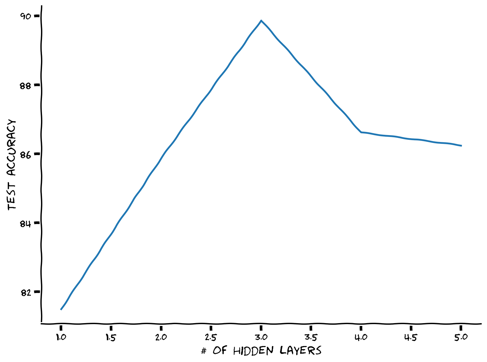
固定されたパラメータ数の制約のもとで最適な隠れ層の数を見つけましょう！
まずはモデルのパラメータ数をカウントする関数が必要です。.parameters()を呼び出してモデルの層を反復処理し、.numel()で層のパラメータ数を数えることができます。また、requires_grad属性を使って訓練可能なパラメータかどうかを確認できます。例えば、

x = torch.ones(10, 5, requires_grad=True)

カウンター関数を定義した後、深さを段階的に増やし、隠れユニット数（すべての隠れ層で同じと仮定）を可能な範囲で反復し、パラメータカウンターを使って全体のパラメータ数がmax_par_countに近くなる隠れユニット数を選びます。

def run_depth_optimizer(max_par_count, max_hidden_layer, device):
  """
  Simulate Depth Optimizer

  Args:
    max_par_count: int
      Maximum number of hidden units in layer of depth optimizer
    max_hidden_layer: int
      Maximum number of hidden layers within depth optimizer
    device: string
      CUDA/GPU if available, CPU otherwise

  Returns:
    hidden_layers: int
      Number of hidden layers in depth optimizer
    test_scores: list
      Log of test scores
  """
  ####################################################################
  # Fill in all missing code below (...),
  # then remove or comment the line below to test your function
  raise NotImplementedError("Define the depth optimizer function")
  ###################################################################

  def count_parameters(model):
    """
    Function to count model parameters

    Args:
      model: instance of Net class
        MLP instance

    Returns:
      par_count: int
        Number of parameters in network
    """
    par_count = 0
    for p in model.parameters():
      if p.requires_grad:
        par_count += ...
    return par_count

  # Number of hidden layers to try
  hidden_layers = ...

  # Test test score list
  test_scores = []

  for hidden_layer in hidden_layers:
    # Initialize the hidden units in each hidden layer to be 1
    hidden_units = np.ones(hidden_layer, dtype=int)

    # Define the the with hidden units equal to 1
    wide_net = Net('ReLU()', X_train.shape[1], hidden_units, K).to(device)
    par_count = count_parameters(wide_net)

    # Increment hidden_units and repeat until the par_count reaches the desired count
    while par_count < max_par_count:
      hidden_units += 1
      wide_net = Net('ReLU()', X_train.shape[1], hidden_units, K).to(device)
      par_count = ...

    # Train it
    criterion = nn.CrossEntropyLoss()
    optimizer = optim.Adam(wide_net.parameters(), lr=1e-3)
    _, test_acc = train_test_classification(wide_net, criterion, optimizer,
                                            train_loader, test_loader,
                                            num_epochs=100, device=device)
    test_scores += [test_acc]

  return hidden_layers, test_scores



set_seed(seed=SEED)
max_par_count = 100
max_hidden_layer = 5
## Uncomment below to test your function
# hidden_layers, test_scores = run_depth_optimizer(max_par_count, max_hidden_layer, DEVICE)
# plt.xlabel('# of hidden layers')
# plt.ylabel('Test accuracy')
# plt.plot(hidden_layers, test_scores)
# plt.show()

解答を見る$

出力例:

# @title Submit your feedback
content_review(f"{feedback_prefix}_Wide_vs_Deep_Exercise")

考えてみよう！1: なぜトレードオフがあるのか？

ここで、最適な隠れ層の数が存在することがわかりました。このシナリオで隠れ層をある点以上に増やすと性能が悪化するのはなぜだと思いますか？

解答を見る$

# @title Submit your feedback
content_review(f"{feedback_prefix}_Wide_vs_Deep_Discussion")

セクション1.1: 幅広いモデルが失敗する場合

前に生成した2つの特徴量を持つスパイラルデータセットを使いましょう。さらに多項式特徴量を追加して（これにより最初の層が広くなります）、単一の線形層を訓練します。隠れ層のない同じMLPネットワークを使うこともできます（ただし、もはやMLPとは呼べませんが）。

多項式の次数を最大 $P=50$ まで追加します。つまり、すべての項 $x_1^n x_2^m$ について $n+m\leq P$ となります。ここで、 $P$ までの多項式特徴量の総数がなぜ以下の式になるかを数学的に証明するのは楽しい演習です:

\text{項数} = \frac{(P+1)(P+2)}{2}

また、nn.Linear層にはバイアス項があるため、次数0の多項式項（定数項）は不要です。したがって、多項式特徴量は1つ少なくなります。

def run_poly_classification(poly_degree, device='cpu', seed=0):
  """
  Helper function to run the above defined polynomial classifier

  Args:
    poly_degree: int
      Degree of the polynomial
    device: string
      CUDA/GPU if available, CPU otherwise
    seed: int
      A non-negative integer that defines the random state. Default is 0.

  Returns:
    num_features: int
      Number of features
  """

  def make_poly_features(poly_degree, X):
    """
    Function to define the number of polynomial features except the bias term

    Args:
      poly_degree: int
        Degree of the polynomial
      X: torch.tensor
        Input data

    Returns:
      num_features: int
        Number of features
      poly_X: torch.tensor
        Polynomial term
    """
    num_features = (poly_degree + 1)*(poly_degree + 2) // 2 - 1
    poly_X = torch.zeros((X.shape[0], num_features))
    count = 0
    for i in range(poly_degree+1):
      for j in range(poly_degree+1):
         # No need to add zero degree since model has biases
        if j + i > 0:
          if j + i <= poly_degree:
            # Define the polynomial term
            poly_X[:, count] = X[:, 0]**i * X [:, 1]**j
            count += 1
    return poly_X, num_features

  poly_X_test, num_features = make_poly_features(poly_degree, X_test)
  poly_X_train, _ = make_poly_features(poly_degree, X_train)

  batch_size = 128

  g_seed = torch.Generator()
  g_seed.manual_seed(seed)
  poly_test_data = TensorDataset(poly_X_test, y_test)
  poly_test_loader = DataLoader(poly_test_data,
                                batch_size=batch_size,
                                shuffle=False,
                                num_workers=1,
                                worker_init_fn=seed_worker,
                                generator=g_seed)

  poly_train_data = TensorDataset(poly_X_train, y_train)
  poly_train_loader = DataLoader(poly_train_data,
                                 batch_size=batch_size,
                                 shuffle=True,
                                 num_workers=1,
                                 worker_init_fn=seed_worker,
                                 generator=g_seed)

  # Define a linear model using MLP class
  poly_net = Net('ReLU()', num_features, [], K).to(device)

  # Train it!
  criterion = nn.CrossEntropyLoss()
  optimizer = optim.Adam(poly_net.parameters(), lr=1e-3)
  _, _ = train_test_classification(poly_net, criterion, optimizer,
                                   poly_train_loader, poly_test_loader,
                                   num_epochs=100, device=DEVICE)
  # Test it
  X_all = sample_grid().to(device)
  poly_X_all, _ = make_poly_features(poly_degree, X_all)
  y_pred = poly_net(poly_X_all.to(device))

  # Plot it
  plot_decision_map(X_all.cpu(), y_pred.cpu(), X_test.cpu(), y_test.cpu())
  plt.show()

  return num_features


set_seed(seed=SEED)
max_poly_degree = 50
num_features = run_poly_classification(max_poly_degree, DEVICE, SEED)
print(f'Number of features: {num_features}')

考えてみよう！1.1: 幅広いモデルは一般化できるか？

このモデルは訓練分布外でもうまく機能していると思いますか？なぜそう思いますか？

解答を見る$

# @title Submit your feedback
content_review(f"{feedback_prefix}_Does_a_wide_model_generalize_well_Discussion")

セクション2: より深いMLP

所要時間の目安: 約55分

# @title Video 2: Case study
from ipywidgets import widgets
from IPython.display import YouTubeVideo
from IPython.display import IFrame
from IPython.display import display


class PlayVideo(IFrame):
  def __init__(self, id, source, page=1, width=400, height=300, **kwargs):
    self.id = id
    if source == 'Bilibili':
      src = f'https://player.bilibili.com/player.html?bvid={id}&page={page}'
    elif source == 'Osf':
      src = f'https://mfr.ca-1.osf.io/render?url=https://osf.io/download/{id}/?direct%26mode=render'
    super(PlayVideo, self).__init__(src, width, height, **kwargs)


def display_videos(video_ids, W=400, H=300, fs=1):
  tab_contents = []
  for i, video_id in enumerate(video_ids):
    out = widgets.Output()
    with out:
      if video_ids[i][0] == 'Youtube':
        video = YouTubeVideo(id=video_ids[i][1], width=W,
                             height=H, fs=fs, rel=0)
        print(f'Video available at https://youtube.com/watch?v={video.id}')
      else:
        video = PlayVideo(id=video_ids[i][1], source=video_ids[i][0], width=W,
                          height=H, fs=fs, autoplay=False)
        if video_ids[i][0] == 'Bilibili':
          print(f'Video available at https://www.bilibili.com/video/{video.id}')
        elif video_ids[i][0] == 'Osf':
          print(f'Video available at https://osf.io/{video.id}')
      display(video)
    tab_contents.append(out)
  return tab_contents


video_ids = [('Youtube', '3g_OJ6dYE8E'), ('Bilibili', 'BV1FL411n7SH')]
tab_contents = display_videos(video_ids, W=854, H=480)
tabs = widgets.Tab()
tabs.children = tab_contents
for i in range(len(tab_contents)):
  tabs.set_title(i, video_ids[i][0])
display(tabs)

# @title Submit your feedback
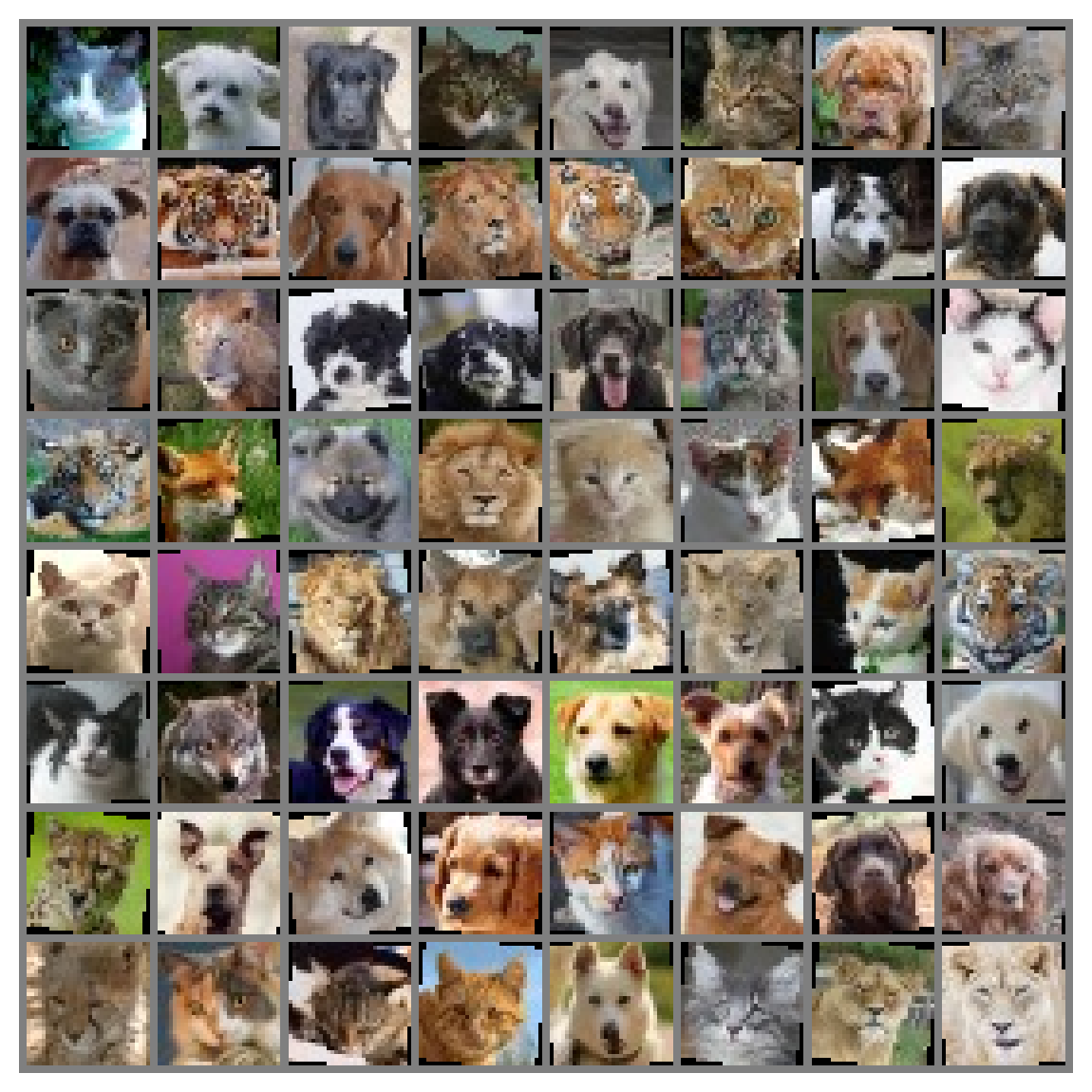
content_review(f"{feedback_prefix}_Case_study_Video")

コーディング演習2: 実世界データセットのデータローダー

データ前処理と拡張を含む最初の実世界データセットローダーを作りましょう！Torchvisionの変換機能を使います。
簡単なデータ拡張として以下のステップを行います:

10度のランダム回転（.RandomRotation）
ランダムな水平反転（.RandomHorizontalFlip）
また、前処理としては:
Pytorchのテンソルを $[0, 1]$ の範囲に変換（.ToTensor）
入力を $[-1, 1]$ の範囲に正規化（.Normalize）

ヒント: 変換についての詳細は公式ドキュメントを参照してください。

def get_data_loaders(batch_size, seed):
  """
  Helper function to get data loaders

  Args:
    batch_size: int
      Batch size
    seed: int
      A non-negative integer that defines the random state.

  Returns:
    img_train_loader: torch.utils.data type
      Combines the train dataset and sampler, and provides an iterable over the given dataset.
    img_test_loader: torch.utils.data type
      Combines the test dataset and sampler, and provides an iterable over the given dataset.
  """
  ####################################################################
  # Fill in all missing code below (...),
  # then remove or comment the line below to test your function
  raise NotImplementedError("Define the get data loaders function")
  ###################################################################

  # Define the transform done only during training
  augmentation_transforms = ...

  # Define the transform done in training and testing (after augmentation)
  mean = (0.5, 0.5, 0.5) # defined sequence of means per channel
  std = (0.5, 0.5, 0.5) # defined sequence of std deviations per channel
  # Note that the transform should normalize each channel: output[channel] = (input[channel] - mean[channel]) / std[channel]
  preprocessing_transforms = ...

  # Compose them together
  train_transform = transforms.Compose(augmentation_transforms + preprocessing_transforms)
  test_transform = transforms.Compose(preprocessing_transforms)

  # Using pathlib to be compatible with all OS's
  data_path = pathlib.Path('.')/'afhq'

  # Define the dataset objects (they can load one by one)
  img_train_dataset = ImageFolder(data_path/'train', transform=train_transform)
  img_test_dataset = ImageFolder(data_path/'val', transform=test_transform)

  g_seed = torch.Generator()
  g_seed.manual_seed(seed)
  # Define the dataloader objects (they can load batch by batch)
  img_train_loader = DataLoader(img_train_dataset,
                                batch_size=batch_size,
                                shuffle=True,
                                worker_init_fn=seed_worker,
                                generator=g_seed)
  # num_workers can be set to higher if running on Colab Pro TPUs to speed up,
  # with more than one worker, it will do multithreading to queue batches
  img_test_loader = DataLoader(img_test_dataset,
                               batch_size=batch_size,
                               shuffle=False,
                               num_workers=1,
                               worker_init_fn=seed_worker,
                               generator=g_seed)

  return img_train_loader, img_test_loader


batch_size = 64
set_seed(seed=SEED)
## Uncomment below to test your function
# img_train_loader, img_test_loader = get_data_loaders(batch_size, SEED)
## get some random training images
# dataiter = iter(img_train_loader)
# images, labels = next(dataiter)
## show images
# imshow(make_grid(images, nrow=8))

解答を見る$

出力例:

# Train it
set_seed(seed=SEED)
net = Net('ReLU()', 3*32*32, [64, 64, 64], 3).to(DEVICE)
criterion = nn.CrossEntropyLoss()
optimizer = optim.Adam(net.parameters(), lr=3e-4)
_, _ = train_test_classification(net, criterion, optimizer,
                                 img_train_loader, img_test_loader,
                                 num_epochs=30, device=DEVICE)

# Visualize the feature map
fc1_weights = net.mlp[0].weight.view(64, 3, 32, 32).detach().cpu()
fc1_weights /= torch.max(torch.abs(fc1_weights))
imshow(make_grid(fc1_weights, nrow=8))

# @title Submit your feedback
content_review(f"{feedback_prefix}_Dataloader_real_world_Exercise")

考えてみよう！2: なぜ最初の層の特徴は高レベルなのか？

3層の深さがあるにもかかわらず、最初の層の特徴マップに明確な動物の顔が見えます。このMLPは階層的な特徴表現を持っていると思いますか？なぜそう思いますか？

解答を見る$

# @title Submit your feedback
content_review(f"{feedback_prefix}_Why_first_layer_features_are_high_level_Discussion")

セクション3: 倫理的側面

所要時間の目安: 約20分

# @title Video 3: Ethics: Hype in AI
from ipywidgets import widgets
from IPython.display import YouTubeVideo
from IPython.display import IFrame
from IPython.display import display


class PlayVideo(IFrame):
  def __init__(self, id, source, page=1, width=400, height=300, **kwargs):
    self.id = id
    if source == 'Bilibili':
      src = f'https://player.bilibili.com/player.html?bvid={id}&page={page}'
    elif source == 'Osf':
      src = f'https://mfr.ca-1.osf.io/render?url=https://osf.io/download/{id}/?direct%26mode=render'
    super(PlayVideo, self).__init__(src, width, height, **kwargs)


def display_videos(video_ids, W=400, H=300, fs=1):
  tab_contents = []
  for i, video_id in enumerate(video_ids):
    out = widgets.Output()
    with out:
      if video_ids[i][0] == 'Youtube':
        video = YouTubeVideo(id=video_ids[i][1], width=W,
                             height=H, fs=fs, rel=0)
        print(f'Video available at https://youtube.com/watch?v={video.id}')
      else:
        video = PlayVideo(id=video_ids[i][1], source=video_ids[i][0], width=W,
                          height=H, fs=fs, autoplay=False)
        if video_ids[i][0] == 'Bilibili':
          print(f'Video available at https://www.bilibili.com/video/{video.id}')
        elif video_ids[i][0] == 'Osf':
          print(f'Video available at https://osf.io/{video.id}')
      display(video)
    tab_contents.append(out)
  return tab_contents


video_ids = [('Youtube', 'ou35QzsKsdc'), ('Bilibili', 'BV1CP4y1s712')]
tab_contents = display_videos(video_ids, W=854, H=480)
tabs = widgets.Tab()
tabs.children = tab_contents
for i in range(len(tab_contents)):
  tabs.set_title(i, video_ids[i][0])
display(tabs)

# @title Submit your feedback
content_review(f"{feedback_prefix}_Ethics_Hype_in_AI_Video")

まとめ

この日の2つ目のチュートリアルでは、MLPをさらに深く掘り下げ、その数学的および実践的な側面を詳しく見てきました。具体的には、深いネットワーク、幅広いネットワーク、そしてそれらが使用する転送関数に依存することについて学びました。また、初期化の重要性についても学び、スマートな初期化のための2つの方法を数学的に解析しました。

# @title Video 4: Outro
from ipywidgets import widgets
from IPython.display import YouTubeVideo
from IPython.display import IFrame
from IPython.display import display


class PlayVideo(IFrame):
  def __init__(self, id, source, page=1, width=400, height=300, **kwargs):
    self.id = id
    if source == 'Bilibili':
      src = f'https://player.bilibili.com/player.html?bvid={id}&page={page}'
    elif source == 'Osf':
      src = f'https://mfr.ca-1.osf.io/render?url=https://osf.io/download/{id}/?direct%26mode=render'
    super(PlayVideo, self).__init__(src, width, height, **kwargs)


def display_videos(video_ids, W=400, H=300, fs=1):
  tab_contents = []
  for i, video_id in enumerate(video_ids):
    out = widgets.Output()
    with out:
      if video_ids[i][0] == 'Youtube':
        video = YouTubeVideo(id=video_ids[i][1], width=W,
                             height=H, fs=fs, rel=0)
        print(f'Video available at https://youtube.com/watch?v={video.id}')
      else:
        video = PlayVideo(id=video_ids[i][1], source=video_ids[i][0], width=W,
                          height=H, fs=fs, autoplay=False)
        if video_ids[i][0] == 'Bilibili':
          print(f'Video available at https://www.bilibili.com/video/{video.id}')
        elif video_ids[i][0] == 'Osf':
          print(f'Video available at https://osf.io/{video.id}')
      display(video)
    tab_contents.append(out)
  return tab_contents


video_ids = [('Youtube', '2sEPw4sSfSw'), ('Bilibili', 'BV1Kb4y1r76G')]
tab_contents = display_videos(video_ids, W=854, H=480)
tabs = widgets.Tab()
tabs.children = tab_contents
for i in range(len(tab_contents)):
  tabs.set_title(i, video_ids[i][0])
display(tabs)

# @title Submit your feedback
content_review(f"{feedback_prefix}_Outro_Video")

ボーナス: 良い初期化の必要性

このセクションでは、深いネットワークの初期化の原理を導出します。重みが大きすぎると、信号の順伝播が混沌となり、誤差勾配の逆伝播が爆発します。一方、重みが小さすぎると、信号の順伝播は秩序的になり、誤差勾配の逆伝播は消失します。初期化の鍵は、秩序と混沌の境界に重みを設定することです。このセクションではその境界を導出し、正しい初期分散の計算方法を示します。

多くの既存の深層学習フレームワークの典型的な初期化スキームは、この秩序と混沌の境界での初期化の原理を暗黙的に利用しています。したがって、このセクションは初回では安全にスキップでき、ボーナスセクションです。

# @title Video 5: Need for Good Initialization
from ipywidgets import widgets
from IPython.display import YouTubeVideo
from IPython.display import IFrame
from IPython.display import display


class PlayVideo(IFrame):
  def __init__(self, id, source, page=1, width=400, height=300, **kwargs):
    self.id = id
    if source == 'Bilibili':
      src = f'https://player.bilibili.com/player.html?bvid={id}&page={page}'
    elif source == 'Osf':
      src = f'https://mfr.ca-1.osf.io/render?url=https://osf.io/download/{id}/?direct%26mode=render'
    super(PlayVideo, self).__init__(src, width, height, **kwargs)


def display_videos(video_ids, W=400, H=300, fs=1):
  tab_contents = []
  for i, video_id in enumerate(video_ids):
    out = widgets.Output()
    with out:
      if video_ids[i][0] == 'Youtube':
        video = YouTubeVideo(id=video_ids[i][1], width=W,
                             height=H, fs=fs, rel=0)
        print(f'Video available at https://youtube.com/watch?v={video.id}')
      else:
        video = PlayVideo(id=video_ids[i][1], source=video_ids[i][0], width=W,
                          height=H, fs=fs, autoplay=False)
        if video_ids[i][0] == 'Bilibili':
          print(f'Video available at https://www.bilibili.com/video/{video.id}')
        elif video_ids[i][0] == 'Osf':
          print(f'Video available at https://osf.io/{video.id}')
      display(video)
    tab_contents.append(out)
  return tab_contents


video_ids = [('Youtube', 'W0V2kwHSuUI'), ('Bilibili', 'BV1Qq4y1H7Px')]
tab_contents = display_videos(video_ids, W=854, H=480)
tabs = widgets.Tab()
tabs.children = tab_contents
for i in range(len(tab_contents)):
  tabs.set_title(i, video_ids[i][0])
display(tabs)

# @title Submit your feedback
content_review(f"{feedback_prefix}_Need_for_Good_Initialization_Bonus_Video")

Xavier初期化

非線形性のない全結合層の出力（例えば隠れ変数） $o_i$ のスケール分布を見てみましょう。この層には $n_{in}$ 個の入力( $x_j$ )とそれに対応する重み $w_{ij}$ があります。出力は次のように表されます。

o_{i} = \sum_{j=1}^{n_\mathrm{in}} w_{ij} x_j

重み $w_{ij}$ はすべて同じ分布から独立にサンプリングされているとします。この分布は平均0、分散 $\sigma^2$ を持つと仮定します。これは分布がガウスである必要はなく、平均と分散が存在すればよいです。入力 $x_j$ も平均0、分散 $\gamma^2$ を持ち、 $w_{ij}$ および互いに独立であると仮定します。この場合、 $o_i$ の平均と分散は次のように計算できます:

\begin{align}
E[o_i] &= $\sum_{j=1}^{n_\mathrm{in}} E$ [ $w_{ij}$ x_j] \ \
&= $\sum_{j=1}^{n_\mathrm{in}} E$ [ $w_{ij}]$ E[x_j] = 0, \ \ \
$\mathrm{Var}$ [o_i] &= $E[o_i^2]$ - ( $E[o_i])^2$ \ \
&= $\sum_{j=1}^{n_\mathrm{in}} E$ [ $w^2_{ij}$ $x^2_j]$ - 0 \ \
&= $\sum_{j=1}^{n_\mathrm{in}} E$ [ $w^2_{ij}]$ $E[x^2_j]$ \ \
&= n_$\mathrm{in} \sigma^2 \gamma^2
\end{align}

分散を一定に保つ一つの方法は $n_{in}\sigma^2=1$ と設定することです。次に逆伝播を考えます。ここでも同様の問題があり、出力に近い層から勾配が伝播します。順伝播と同様の理由で、勾配の分散が爆発しないためには $n_{out}\sigma^2=1$ を満たす必要があります。ここで $n_{out}$ はこの層の出力数です。両方を同時に満たすことはできないため、代わりに次の条件を満たすようにします:

\begin{align}
$\frac{1}{2} (n_\mathrm{in} + n_\mathrm{out}) \sigma^2 = 1 \text{ または同値に }
\sigma = \sqrt{\frac{2}{n_\mathrm{in} + n_\mathrm{out}}}
\end{align}

これが現在標準的かつ実用的に有益なXavier初期化の理論的根拠であり、作成者の一人の名前にちなんでいますGlorot and Bengio, 2010。通常、Xavier初期化は平均0、分散 $\sigma^2=\frac{2}{(n_{in}+n_{out})}$ のガウス分布から重みをサンプリングします。

w_{ij} \sim \mathcal{N} \left (\mu=0, \sigma=\sqrt{\frac{2}{(n_{in}+n_{out})}} \right)

また、Xavierの直感を用いて一様分布から重みをサンプリングする場合の分散も選べます。一様分布 $\mathcal{U}(−a,a)$ の分散は $\frac{a^2}{3}$ です。これを条件に代入すると、次のように初期化することが推奨されます。

w_{ij} \sim \mathcal{U} \left(-\sqrt{\frac{6}{n_\mathrm{in} + n_\mathrm{out}}}, \sqrt{\frac{6}{n_\mathrm{in} + n_\mathrm{out}}}\right)

この説明は主にこちら$から引用しています。

初期化とその違いについてもっと知りたい場合はこちらを参照してください。

転送関数を考慮した初期化

LeakyReLUの最適なゲインを同様の手順で導出しましょう。

LeakyReLUは数学的に次のように表されます:

f(x)=\left\{ \begin{array}{ll} \alpha \cdot x & \text { for } x<0 \\ x & \text { for } x \geq 0 \end{array}\right.

ここで $\alpha$ は負の傾きの角度を制御します。

この活性化関数を持つ単一層を考えると、

\begin{align}
$o_{i}$ &= $\sum_{j=1}^{n_\mathrm{in}} w_{ij} x_j$ \
$z_{i}$ &= f $\left( o_{i} \right) \end{align}$

ここで $z_i$ はノード $i$ の活性化を表します。

出力の期待値は依然として0、すなわち $\mathbb{E}[f(o_i)=0]$ ですが、分散は変わり、 $P(x < 0) = 0.5$ と仮定すると、

\begin{align}
$\mathrm{Var}$ [ $f(o_i)]$ &= $\mathbb{E}$ [ $f(o_i)^2]$ - $\left( \mathbb{E}$ [ $f(o_i)]$ $\right)^{2}$ \ \
&= $\frac{\mathrm{Var}$ [o_i] + $\alpha^2 \mathrm{Var}$ [ $o_i]}{2}$ \ \
&= $\frac{1+\alpha^2}{2}n_\mathrm{in} \sigma^2 \gamma^2 \end{align}$

ここで $\gamma$ は入力 $x_j$ の分散、 $\sigma$ は重み $w_{ij}$ の分散です。

したがって、前述の導出に従うと、

\sigma = gain\sqrt{\frac{2}{n_\mathrm{in} + n_\mathrm{out}}}, \, \text{ただし} \,\, gain = \sqrt{\frac{2}{1+\alpha^2}}

導出された $\sigma$ の式からわかるように、選択する転送関数は重みの分布の分散に関連しています。LeakyReLUの負の傾き $\alpha$ が大きくなると $gain$ は小さくなり、重みの分布は狭くなります。一方、 $\alpha$ が小さくなると重みの分布は広くなります。例えば、重みは平均0、分散 $\sigma^2$ の正規分布からサンプリングして初期化します。

Leaky ReLUを用いたXavier初期化の最適ゲイン

時間があまりないと思うので、ここで何が起きているか説明します。理論的な初期化ゲインを導出しましたが、実際にそれが成り立つかどうかは疑問です。ここでは様々なゲインを試し、経験的な最適値が理論値と一致するかを確認します！

時間があれば、mode引数を変えて初期重みのサンプリング分布を一様分布に変更することもできます。

N = 10  # Number of trials
gains = np.linspace(1/N, 3.0, N)
test_accs = []
train_accs = []
mode = 'uniform'
for gain in gains:
  print(f'\ngain: {gain:.2f}')

  def init_weights(m, mode='normal'):
    if type(m) == nn.Linear:
      if mode == 'normal':
        torch.nn.init.xavier_normal_(m.weight, gain)
      elif mode == 'uniform':
        torch.nn.init.xavier_uniform_(m.weight, gain)
      else:
        print("No specific mode selected. Please choose `normal` or `uniform`")

  negative_slope = 0.1
  actv = f'LeakyReLU({negative_slope})'
  set_seed(seed=SEED)
  net = Net(actv, 3*32*32, [128, 64, 32], 3).to(DEVICE)
  net.apply(init_weights)
  criterion = nn.CrossEntropyLoss()

  optimizer = optim.SGD(net.parameters(), lr=1e-2)
  train_acc, test_acc = train_test_classification(net, criterion, optimizer,
                                                  img_train_loader,
                                                  img_test_loader,
                                                  num_epochs=1,
                                                  verbose=True,
                                                  device=DEVICE)
  test_accs += [test_acc]
  train_accs += [train_acc]

結果をプロットしてみましょう！

# Find the gain that leads to the highest accuracy
best_gain = gains[np.argmax(train_accs)]

# Calculate the theoretical gain
theoretical_gain = np.sqrt(2.0 / (1 + negative_slope ** 2))

plt.figure()
plt.plot(gains, test_accs, label='Test accuracy', marker='.', alpha=0.6)
plt.plot(gains, train_accs, label='Train accuracy', marker='.', alpha=0.6)
plt.scatter(best_gain, max(train_accs),
            label=f'best gain={best_gain:.2f}',
            c='k', marker ='x', linewidths=2)
plt.scatter(theoretical_gain, max(train_accs),
            label=f'theoretical gain={theoretical_gain:.2f}',
            c='g', marker ='x', linewidths=2)
plt.ylabel('Accuracy (%)')
plt.xlabel('gain')
plt.legend()
plt.show()