チュートリアル 1: 生物学的ニューラルネットワーク vs. 人工ニューラルネットワーク

第1週、第3日目: 多層パーセプトロン

Neuromatch Academyによる

コンテンツ作成者: Arash Ash, Surya Ganguli

コンテンツレビュアー: Saeed Salehi, Felix Bartsch, Yu-Fang Yang, Antoine De Comite, Melvin Selim Atay, Kelson Shilling-Scrivo

コンテンツ編集者: Gagana B, Kelson Shilling-Scrivo, Spiros Chavlis

制作編集者: Anoop Kulkarni, Kelson Shilling-Scrivo, Gagana B, Spiros Chavlis

チュートリアルの目的

このチュートリアルでは、多層パーセプトロン（MLP）について探求します。MLPは、深層学習の基本を学ぶために使える最も扱いやすいモデルの一つ（その柔軟性ゆえに）と言えます。ここでは、MLPが以下の理由で優れていることを学びます：

生物学的ネットワークに似ている
関数近似に優れている
PyTorchで実装されている方法

# @title Tutorial slides
from IPython.display import IFrame
link_id = "4ye56"
print(f"If you want to download the slides: https://osf.io/download/{link_id}/")
IFrame(src=f"https://mfr.ca-1.osf.io/render?url=https://osf.io/{link_id}/?direct%26mode=render%26action=download%26mode=render", width=854, height=480)

セットアップ

このノートブックはGPUを使用しません！

# @title Install and import feedback gadget


from vibecheck import DatatopsContentReviewContainer
def content_review(notebook_section: str):
    return DatatopsContentReviewContainer(
        "",  # No text prompt
        notebook_section,
        {
            "url": "https://pmyvdlilci.execute-api.us-east-1.amazonaws.com/klab",
            "name": "neuromatch_dl",
            "user_key": "f379rz8y",
        },
    ).render()


feedback_prefix = "W1D3_T1"

# Imports
import random

import torch
import numpy as np
import matplotlib.pyplot as plt

import torch.nn as nn
import torch.optim as optim
from tqdm.auto import tqdm
from IPython.display import display
from torch.utils.data import DataLoader, TensorDataset

# @title Figure settings
import logging
logging.getLogger('matplotlib.font_manager').disabled = True

import ipywidgets as widgets  # Interactive display
%config InlineBackend.figure_format = 'retina'
plt.style.use("https://raw.githubusercontent.com/NeuromatchAcademy/content-creation/main/nma.mplstyle")

# @title Plotting functions

def imshow(img):
  """
  Helper function to plot unnormalised image

  Args:
    img: torch.tensor
      Image to be displayed

  Returns:
    Nothing
  """
  img = img / 2 + 0.5  # Unnormalize
  npimg = img.numpy()
  plt.imshow(np.transpose(npimg, (1, 2, 0)))
  plt.axis(False)
  plt.show()


def plot_function_approximation(x, relu_acts, y_hat):
  """
  Helper function to plot ReLU activations and
  function approximations

  Args:
    x: torch.tensor
      Incoming Data
    relu_acts: torch.tensor
      Computed ReLU activations for each point along the x axis (x)
    y_hat: torch.tensor
      Estimated labels/class predictions
      Weighted sum of ReLU activations for every point along x axis

  Returns:
    Nothing
  """
  fig, axes = plt.subplots(2, 1)

  # Plot ReLU Activations
  axes[0].plot(x, relu_acts.T);
  axes[0].set(xlabel='x',
              ylabel='Activation',
              title='ReLU Activations - Basis Functions')
  labels = [f"ReLU {i + 1}" for i in range(relu_acts.shape[0])]
  axes[0].legend(labels, ncol = 2)

  # Plot Function Approximation
  axes[1].plot(x, torch.sin(x), label='truth')
  axes[1].plot(x, y_hat, label='estimated')
  axes[1].legend()
  axes[1].set(xlabel='x',
              ylabel='y(x)',
              title='Function Approximation')

  plt.tight_layout()
  plt.show()

# @title Set random seed

# @markdown Executing `set_seed(seed=seed)` you are setting the seed

# For DL its critical to set the random seed so that students can have a
# baseline to compare their results to expected results.
# Read more here: https://pytorch.org/docs/stable/notes/randomness.html

# Call `set_seed` function in the exercises to ensure reproducibility.
import random
import torch

def set_seed(seed=None, seed_torch=True):
  """
  Function that controls randomness. NumPy and random modules must be imported.

  Args:
    seed : Integer
      A non-negative integer that defines the random state. Default is `None`.
    seed_torch : Boolean
      If `True` sets the random seed for pytorch tensors, so pytorch module
      must be imported. Default is `True`.

  Returns:
    Nothing.
  """
  if seed is None:
    seed = np.random.choice(2 ** 32)
  random.seed(seed)
  np.random.seed(seed)
  if seed_torch:
    torch.manual_seed(seed)
    torch.cuda.manual_seed_all(seed)
    torch.cuda.manual_seed(seed)
    torch.backends.cudnn.benchmark = False
    torch.backends.cudnn.deterministic = True

  print(f'Random seed {seed} has been set.')


# In case that `DataLoader` is used
def seed_worker(worker_id):
  """
  DataLoader will reseed workers following randomness in
  multi-process data loading algorithm.

  Args:
    worker_id: integer
      ID of subprocess to seed. 0 means that
      the data will be loaded in the main process
      Refer: https://pytorch.org/docs/stable/data.html#data-loading-randomness for more details

  Returns:
    Nothing
  """
  worker_seed = torch.initial_seed() % 2**32
  np.random.seed(worker_seed)
  random.seed(worker_seed)

# @title Set device (GPU or CPU). Execute `set_device()`
# especially if torch modules used.

# Inform the user if the notebook uses GPU or CPU.
# NOTE: This is mostly a GPU free tutorial.

def set_device():
  """
  Set the device. CUDA if available, CPU otherwise

  Args:
    None

  Returns:
    Nothing
  """
  device = "cuda" if torch.cuda.is_available() else "cpu"
  if device != "cuda":
    print("GPU is not enabled in this notebook. \n"
          "If you want to enable it, in the menu under `Runtime` -> \n"
          "`Hardware accelerator.` and select `GPU` from the dropdown menu")
  else:
    print("GPU is enabled in this notebook. \n"
          "If you want to disable it, in the menu under `Runtime` -> \n"
          "`Hardware accelerator.` and select `None` from the dropdown menu")

  return device

SEED = 2021
set_seed(seed=SEED)
DEVICE = set_device()

セクション0: MLPの紹介

# @title Video 0: Introduction
from ipywidgets import widgets
from IPython.display import YouTubeVideo
from IPython.display import IFrame
from IPython.display import display


class PlayVideo(IFrame):
  def __init__(self, id, source, page=1, width=400, height=300, **kwargs):
    self.id = id
    if source == 'Bilibili':
      src = f'https://player.bilibili.com/player.html?bvid={id}&page={page}'
    elif source == 'Osf':
      src = f'https://mfr.ca-1.osf.io/render?url=https://osf.io/download/{id}/?direct%26mode=render'
    super(PlayVideo, self).__init__(src, width, height, **kwargs)


def display_videos(video_ids, W=400, H=300, fs=1):
  tab_contents = []
  for i, video_id in enumerate(video_ids):
    out = widgets.Output()
    with out:
      if video_ids[i][0] == 'Youtube':
        video = YouTubeVideo(id=video_ids[i][1], width=W,
                             height=H, fs=fs, rel=0)
        print(f'Video available at https://youtube.com/watch?v={video.id}')
      else:
        video = PlayVideo(id=video_ids[i][1], source=video_ids[i][0], width=W,
                          height=H, fs=fs, autoplay=False)
        if video_ids[i][0] == 'Bilibili':
          print(f'Video available at https://www.bilibili.com/video/{video.id}')
        elif video_ids[i][0] == 'Osf':
          print(f'Video available at https://osf.io/{video.id}')
      display(video)
    tab_contents.append(out)
  return tab_contents


video_ids = [('Youtube', 'Gh0KYl7ViAc'), ('Bilibili', 'BV1E3411r7TL')]
tab_contents = display_videos(video_ids, W=854, H=480)
tabs = widgets.Tab()
tabs.children = tab_contents
for i in range(len(tab_contents)):
  tabs.set_title(i, video_ids[i][0])
display(tabs)

# @title Submit your feedback
content_review(f"{feedback_prefix}_Introduction_Video")

セクション1: MLPが必要な理由

所要時間の目安: 約35分

# @title Video 1: Universal Approximation Theorem
from ipywidgets import widgets
from IPython.display import YouTubeVideo
from IPython.display import IFrame
from IPython.display import display


class PlayVideo(IFrame):
  def __init__(self, id, source, page=1, width=400, height=300, **kwargs):
    self.id = id
    if source == 'Bilibili':
      src = f'https://player.bilibili.com/player.html?bvid={id}&page={page}'
    elif source == 'Osf':
      src = f'https://mfr.ca-1.osf.io/render?url=https://osf.io/download/{id}/?direct%26mode=render'
    super(PlayVideo, self).__init__(src, width, height, **kwargs)


def display_videos(video_ids, W=400, H=300, fs=1):
  tab_contents = []
  for i, video_id in enumerate(video_ids):
    out = widgets.Output()
    with out:
      if video_ids[i][0] == 'Youtube':
        video = YouTubeVideo(id=video_ids[i][1], width=W,
                             height=H, fs=fs, rel=0)
        print(f'Video available at https://youtube.com/watch?v={video.id}')
      else:
        video = PlayVideo(id=video_ids[i][1], source=video_ids[i][0], width=W,
                          height=H, fs=fs, autoplay=False)
        if video_ids[i][0] == 'Bilibili':
          print(f'Video available at https://www.bilibili.com/video/{video.id}')
        elif video_ids[i][0] == 'Osf':
          print(f'Video available at https://osf.io/{video.id}')
      display(video)
    tab_contents.append(out)
  return tab_contents


video_ids = [('Youtube', 'tg8HHKo1aH4'), ('Bilibili', 'BV1SP4y147Uv')]
tab_contents = display_videos(video_ids, W=854, H=480)
tabs = widgets.Tab()
tabs.children = tab_contents
for i in range(len(tab_contents)):
  tabs.set_title(i, video_ids[i][0])
display(tabs)

# @title Submit your feedback
content_review(f"{feedback_prefix}_Universal_Approximation_Theorem_Video")

コーディング演習1: ReLUを用いた関数近似

ユニバーサル近似定理を通じて、1つの隠れ層を持つMLPであれば任意の滑らかな関数を近似できることを学びました！ここではReLU活性化関数を使って、手動で正弦関数をフィットさせてみましょう。

正弦関数を、傾き1のReLUの線形結合（重み付き和）で近似します。ReLUの屈曲点（0から線形への変化点）を決めるバイアス項と、それぞれのReLUにかける重みを決定する必要があります。アイデアは、新しいサンプルの方向に傾きが変わるように重みを反復的に設定することです。

まず、torch.sin関数を使って正弦関数から「訓練データ」を生成します。

>>> import torch
>>> torch.manual_seed(2021)
<torch._C.Generator object at 0x7f8734c83830>
>>> a = torch.randn(5)
>>> print(a)
tensor([ 2.2871,  0.6413, -0.8615, -0.3649, -0.6931])
>>> torch.sin(a)
tensor([ 0.7542,  0.5983, -0.7588, -0.3569, -0.6389])

これらの点を使って関数近似の学習を行います。訓練データは10点あるので、ReLUは9個用意します（最後のデータ点の右側にモデル化するものがないため、ReLUは不要です）。

まず各ReLUのバイアス項を決め、以下の式で各ReLUの活性化を計算します：

y(x) = \text{max}(0, x+b)

次に、線形結合が目的の関数を近似するように、各ReLUの重みを正しく決定します。

def approximate_function(x_train, y_train):
  """
  Function to compute and combine ReLU activations

  Args:
    x_train: torch.tensor
      Training data
    y_train: torch.tensor
      Ground truth labels corresponding to training data

  Returns:
    relu_acts: torch.tensor
      Computed ReLU activations for each point along the x axis (x)
    y_hat: torch.tensor
      Estimated labels/class predictions
      Weighted sum of ReLU activations for every point along x axis
    x: torch.tensor
      x-axis points
  """
  ####################################################################
  # Fill in missing code below (...),
  # then remove or comment the line below to test your function
  raise NotImplementedError("Complete approximate_function!")
  ####################################################################

  # Number of relus
  n_relus = x_train.shape[0] - 1

  # x axis points (more than x train)
  x = torch.linspace(torch.min(x_train), torch.max(x_train), 1000)

  ## COMPUTE RELU ACTIVATIONS

  # First determine what bias terms should be for each of `n_relus` ReLUs
  b = ...

  # Compute ReLU activations for each point along the x axis (x)
  relu_acts = torch.zeros((n_relus, x.shape[0]))

  for i_relu in range(n_relus):
    relu_acts[i_relu, :] = torch.relu(x + b[i_relu])

  ## COMBINE RELU ACTIVATIONS

  # Set up weights for weighted sum of ReLUs
  combination_weights = torch.zeros((n_relus, ))

  # Figure out weights on each ReLU
  prev_slope = 0
  for i in range(n_relus):
    delta_x = x_train[i+1] - x_train[i]
    slope = (y_train[i+1] - y_train[i]) / delta_x
    combination_weights[i] = ...
    prev_slope = slope

  # Get output of weighted sum of ReLU activations for every point along x axis
  y_hat = ...

  return y_hat, relu_acts, x



# Make training data from sine function
N_train = 10
x_train = torch.linspace(0, 2*np.pi, N_train).view(-1, 1)
y_train = torch.sin(x_train)

## Uncomment the lines below to test your function approximation
# y_hat, relu_acts, x = approximate_function(x_train, y_train)
# plot_function_approximation(x, relu_acts, y_hat)

解答を見る$

出力例:

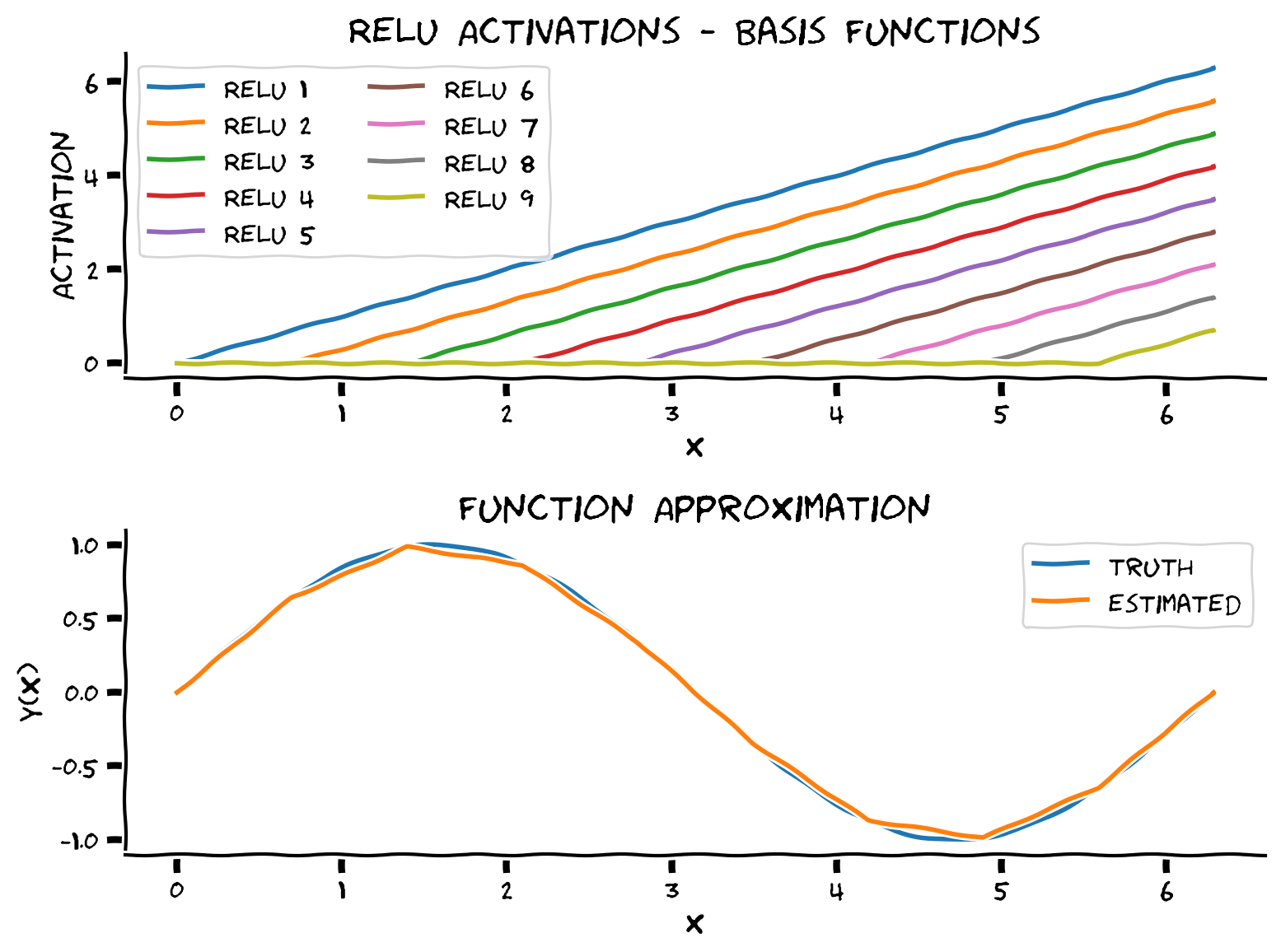
上のパネルに示されているように、傾きが同じ10個のシフトされたReLUを得ています。これらはMLPが関数空間を張るために使う基底関数であり、MLPはこれらのReLUの線形結合を見つけることになります。

# @title Submit your feedback
content_review(f"{feedback_prefix}_Function_approximation_with_ReLU_Exercise")

セクション2: PyTorchにおけるMLP

所要時間の目安: 約1時間20分

# @title Video 2: Building MLPs in PyTorch
from ipywidgets import widgets
from IPython.display import YouTubeVideo
from IPython.display import IFrame
from IPython.display import display


class PlayVideo(IFrame):
  def __init__(self, id, source, page=1, width=400, height=300, **kwargs):
    self.id = id
    if source == 'Bilibili':
      src = f'https://player.bilibili.com/player.html?bvid={id}&page={page}'
    elif source == 'Osf':
      src = f'https://mfr.ca-1.osf.io/render?url=https://osf.io/download/{id}/?direct%26mode=render'
    super(PlayVideo, self).__init__(src, width, height, **kwargs)


def display_videos(video_ids, W=400, H=300, fs=1):
  tab_contents = []
  for i, video_id in enumerate(video_ids):
    out = widgets.Output()
    with out:
      if video_ids[i][0] == 'Youtube':
        video = YouTubeVideo(id=video_ids[i][1], width=W,
                             height=H, fs=fs, rel=0)
        print(f'Video available at https://youtube.com/watch?v={video.id}')
      else:
        video = PlayVideo(id=video_ids[i][1], source=video_ids[i][0], width=W,
                          height=H, fs=fs, autoplay=False)
        if video_ids[i][0] == 'Bilibili':
          print(f'Video available at https://www.bilibili.com/video/{video.id}')
        elif video_ids[i][0] == 'Osf':
          print(f'Video available at https://osf.io/{video.id}')
      display(video)
    tab_contents.append(out)
  return tab_contents


video_ids = [('Youtube', 'XtwLnaYJ7uc'), ('Bilibili', 'BV1zh411z7LY')]
tab_contents = display_videos(video_ids, W=854, H=480)
tabs = widgets.Tab()
tabs.children = tab_contents
for i in range(len(tab_contents)):
  tabs.set_title(i, video_ids[i][0])
display(tabs)

# @title Submit your feedback
content_review(f"{feedback_prefix}_Building_MLPs_in_PyTorch_Video")

前のセクションでは、MLPを使って任意の滑らかな関数を近似する関数を実装しました。リプシッツ連続性を用いて、この近似が数学的に正しいことを証明できることも見ました。MLPは非常に興味深いですが、設計の詳細に入る前に、MLPの基本用語（層、ニューロン、深さ、幅、重み、バイアス、活性化関数）に慣れましょう。これらの概念を身につけた上で、入力サイズ、隠れ層の数、出力サイズを指定してMLPを設計できるようになります。

コーディング演習 2: Pytorchで汎用的なMLPを実装する

目的は以下の特性を持つMLPを設計することです:

任意の入力（1D、2Dなど）に対応する
nn.Sequential() と $add_module()$ 関数を使って任意の数の隠れ層を構築する
すべての隠れ層で同じ活性化関数（例: Leaky ReLU）を使用する

Leaky ReLU は以下の数式で表されます:

\begin{align}
$\text{LeakyReLU}(x)$ &= $\text{max}(0,x) + \text{negative_slope} \cdot \text{min}(0, x)$ \
&=
$\left$ {
\begin{array}{ll}
x & ,; $\text{if}$ ; x $\ge 0$ \
$\text{negative_slope} \cdot x$ & ,; $\text{otherwise} \end{array} \right$ .
\end{align}

class Net(nn.Module):
  """
  Initialize MLP Network
  """

  def __init__(self, actv, input_feature_num, hidden_unit_nums, output_feature_num):
    """
    Initialize MLP Network parameters

    Args:
      actv: string
        Activation function
      input_feature_num: int
        Number of input features
      hidden_unit_nums: list
        Number of units per hidden layer, list of integers
      output_feature_num: int
        Number of output features

    Returns:
      Nothing
    """
    super(Net, self).__init__()
    self.input_feature_num = input_feature_num # Save the input size for reshaping later
    self.mlp = nn.Sequential() # Initialize layers of MLP

    in_num = input_feature_num # Initialize the temporary input feature to each layer
    for i in range(len(hidden_unit_nums)): # Loop over layers and create each one

      ####################################################################
      # Fill in missing code below (...),
      # Then remove or comment the line below to test your function
      raise NotImplementedError("Create MLP Layer")
      ####################################################################

      out_num = hidden_unit_nums[i] # Assign the current layer hidden unit from list
      layer = ... # Use nn.Linear to define the layer
      in_num = out_num # Assign next layer input using current layer output
      self.mlp.add_module('Linear_%d'%i, layer) # Append layer to the model with a name

      actv_layer = eval('nn.%s'%actv) # Assign activation function (eval allows us to instantiate object from string)
      self.mlp.add_module('Activation_%d'%i, actv_layer) # Append activation to the model with a name

    out_layer = nn.Linear(in_num, output_feature_num) # Create final layer
    self.mlp.add_module('Output_Linear', out_layer) # Append the final layer

  def forward(self, x):
    """
    Simulate forward pass of MLP Network

    Args:
      x: torch.tensor
        Input data

    Returns:
      logits: Instance of MLP
        Forward pass of MLP
    """
    # Reshape inputs to (batch_size, input_feature_num)
    # Just in case the input vector is not 2D, like an image!
    x = x.view(-1, self.input_feature_num)

    ####################################################################
    # Fill in missing code below (...),
    # then remove or comment the line below to test your function
    raise NotImplementedError("Run MLP model")
    ####################################################################

    logits = ... # Forward pass of MLP
    return logits



input = torch.zeros((100, 2))
## Uncomment below to create network and test it on input
# net = Net(actv='LeakyReLU(0.1)', input_feature_num=2, hidden_unit_nums=[100, 10, 5], output_feature_num=1).to(DEVICE)
# y = net(input.to(DEVICE))
# print(f'The output shape is {y.shape} for an input of shape {input.shape}')

解答を見る$

入力の形状が torch.Size([100, 2]) のとき、出力の形状は torch.Size([100, 1]) です

# @title Submit your feedback
content_review(f"{feedback_prefix}_Implement_a_general_purpose_MLP_in_PyTorch_Exercise")

セクション 2.1: MLPによる分類

# @title Video 3: Cross Entropy
from ipywidgets import widgets
from IPython.display import YouTubeVideo
from IPython.display import IFrame
from IPython.display import display


class PlayVideo(IFrame):
  def __init__(self, id, source, page=1, width=400, height=300, **kwargs):
    self.id = id
    if source == 'Bilibili':
      src = f'https://player.bilibili.com/player.html?bvid={id}&page={page}'
    elif source == 'Osf':
      src = f'https://mfr.ca-1.osf.io/render?url=https://osf.io/download/{id}/?direct%26mode=render'
    super(PlayVideo, self).__init__(src, width, height, **kwargs)


def display_videos(video_ids, W=400, H=300, fs=1):
  tab_contents = []
  for i, video_id in enumerate(video_ids):
    out = widgets.Output()
    with out:
      if video_ids[i][0] == 'Youtube':
        video = YouTubeVideo(id=video_ids[i][1], width=W,
                             height=H, fs=fs, rel=0)
        print(f'Video available at https://youtube.com/watch?v={video.id}')
      else:
        video = PlayVideo(id=video_ids[i][1], source=video_ids[i][0], width=W,
                          height=H, fs=fs, autoplay=False)
        if video_ids[i][0] == 'Bilibili':
          print(f'Video available at https://www.bilibili.com/video/{video.id}')
        elif video_ids[i][0] == 'Osf':
          print(f'Video available at https://osf.io/{video.id}')
      display(video)
    tab_contents.append(out)
  return tab_contents


video_ids = [('Youtube', 'N8pVCbTlves'), ('Bilibili', 'BV1Ag41177mB')]
tab_contents = display_videos(video_ids, W=854, H=480)
tabs = widgets.Tab()
tabs.children = tab_contents
for i in range(len(tab_contents)):
  tabs.set_title(i, video_ids[i][0])
display(tabs)

# @title Submit your feedback
content_review(f"{feedback_prefix}_Cross_Entropy_Video")

多クラス分類において、N 個のサンプルと C クラスに対してそのまま使える主な損失関数は以下の通りです。

CrossEntropyLoss:
この基準は、形状が (N, C) の予測値 x のバッチと、各 N サンプルに対してクラスインデックスが $[0, C-1]$ の範囲にあるターゲット（ラベル）を期待します。したがって、ラベルのバッチは形状 (N,) となります。クラスの重み付けや無視するクラスなどのオプションパラメータもあります。詳細はPyTorchのドキュメントこちらをご覧ください。さらに、CrossEntropyLossの適切な使いどころについてはこちらで学べます。

サンプル $i$ のCrossEntropyLossを得るには、まず $-\log(\text{softmax}(x))$ を計算し、次に $\text {labels}_i$ に対応する要素を損失として取ることができます。しかし、数値的安定性のために、より安定した同等の形で実装しています。

\operatorname{loss}(x_i, \text {labels}_i)=-\log \left(\frac{\exp (x[\text {labels}_i])}{\sum_{j} \exp (x[j])}\right)=-x_i[\text {labels}_i]+\log \left(\sum_{j=1}^C \exp (x_i[j])\right)

コーディング演習 2.1: バッチクロスエントロピー損失の実装

復習すると、バッチ学習を行うため、以下を受け取る損失関数が欲しいです：

形状が (N, C) の予測値のバッチ x
形状が (N,) で、値が 0 から C-1 の範囲の labels のバッチ

以下の式に従って計算される平均損失 $L$ を返します：

\begin{align}
$\text{loss}(x_i, \text {labels}_i)$ &= -x_i[ $\text {labels}_i$ ]+ $\log \left(\sum_{j=1}^C \exp (x_i$ [j]) $\right)$ \
L &= $\frac{1}{N} \sum_{i=1}^{N}{\text{loss}(x_i, \text {labels}_i)} \end{align}$

手順：

インデックス操作を使ってラベルに対応するクラスの予測値を取得する（すなわち、 $x_i[\text { labels }_i]$ ）
torch.log() と torch.exp() を使ってループなしで $loss(x_i, \text { labels }_i)$ ベクトル（losses）を計算する
損失ベクトルの平均を返す

def cross_entropy_loss(x, labels):
  """
  Helper function to compute cross entropy loss

  Args:
    x: torch.tensor
      Model predictions we'd like to evaluate using labels
    labels: torch.tensor
      Ground truth

  Returns:
    avg_loss: float
      Average of the loss vector
  """
  x_of_labels = torch.zeros(len(labels))
  ####################################################################
  # Fill in missing code below (...),
  # then remove or comment the line below to test your function
  raise NotImplementedError("Cross Entropy Loss")
  ####################################################################
  # 1. Prediction for each class corresponding to the label
  for i, label in enumerate(labels):
    x_of_labels[i] = x[i, label]
  # 2. Loss vector for the batch
  losses = ...
  # 3. Return the average of the loss vector
  avg_loss = ...

  return avg_loss



labels = torch.tensor([0, 1])
x = torch.tensor([[10.0, 1.0, -1.0, -20.0],  # Correctly classified
                  [10.0, 10.0, 2.0, -10.0]])  # Not correctly classified
CE = nn.CrossEntropyLoss()
pytorch_loss = CE(x, labels).item()
## Uncomment below to test your function
# our_loss = cross_entropy_loss(x, labels).item()
# print(f'Our CE loss: {our_loss:0.8f}, Pytorch CE loss: {pytorch_loss:0.8f}')
# print(f'Difference: {np.abs(our_loss - pytorch_loss):0.8f}')

解答を見る$

私たちの CE 損失: 0.34672737, Pytorch の CE 損失: 0.34672749
差分: 0.00000012

# @title Submit your feedback
content_review(f"{feedback_prefix}_Implement_Batch_Cross_Entropy_Loss_Exercise")

セクション 2.2: スパイラル分類データセット

これらの損失関数を最適化し始める前に、データセットが必要です！

この見た目が複雑な方程式を分類データセットに変換しましょう

\begin{array}{c} X_{k}(t)=t\left(\begin{array}{c} \sin \left[\frac{2 \pi}{K}\left(2 t+k-1\right)\right]+\mathcal{N}\left(0, \sigma\right) \\ \cos \left[\frac{2 \pi}{K}\left(2 t+k-1\right)\right]+\mathcal{N}\left(0, \sigma\right) \end{array}\right) \end{array}, \quad 0 \leq t \leq 1, \quad k=1, \ldots, K

def create_spiral_dataset(K, sigma, N):
  """
  Function to simulate spiral dataset

  Args:
    K: int
      Number of classes
    sigma: float
      Standard deviation
    N: int
      Number of data points

  Returns:
    X: torch.tensor
      Spiral data
    y: torch.tensor
      Corresponding ground truth
  """

  # Initialize t, X, y
  t = torch.linspace(0, 1, N)
  X = torch.zeros(K*N, 2)
  y = torch.zeros(K*N)

  # Create data
  for k in range(K):
    X[k*N:(k+1)*N, 0] = t*(torch.sin(2*np.pi/K*(2*t+k)) + sigma*torch.randn(N))
    X[k*N:(k+1)*N, 1] = t*(torch.cos(2*np.pi/K*(2*t+k)) + sigma*torch.randn(N))
    y[k*N:(k+1)*N] = k

  return X, y


# Set parameters
K = 4
sigma = 0.16
N = 1000

set_seed(seed=SEED)
X, y = create_spiral_dataset(K, sigma, N)
plt.scatter(X[:, 0], X[:, 1], c = y)
plt.xlabel('x1')
plt.ylabel('x2')
plt.show()

セクション 2.3: トレーニングと評価

# @title Video 4: Training and Evaluating an MLP
from ipywidgets import widgets
from IPython.display import YouTubeVideo
from IPython.display import IFrame
from IPython.display import display


class PlayVideo(IFrame):
  def __init__(self, id, source, page=1, width=400, height=300, **kwargs):
    self.id = id
    if source == 'Bilibili':
      src = f'https://player.bilibili.com/player.html?bvid={id}&page={page}'
    elif source == 'Osf':
      src = f'https://mfr.ca-1.osf.io/render?url=https://osf.io/download/{id}/?direct%26mode=render'
    super(PlayVideo, self).__init__(src, width, height, **kwargs)


def display_videos(video_ids, W=400, H=300, fs=1):
  tab_contents = []
  for i, video_id in enumerate(video_ids):
    out = widgets.Output()
    with out:
      if video_ids[i][0] == 'Youtube':
        video = YouTubeVideo(id=video_ids[i][1], width=W,
                             height=H, fs=fs, rel=0)
        print(f'Video available at https://youtube.com/watch?v={video.id}')
      else:
        video = PlayVideo(id=video_ids[i][1], source=video_ids[i][0], width=W,
                          height=H, fs=fs, autoplay=False)
        if video_ids[i][0] == 'Bilibili':
          print(f'Video available at https://www.bilibili.com/video/{video.id}')
        elif video_ids[i][0] == 'Osf':
          print(f'Video available at https://osf.io/{video.id}')
      display(video)
    tab_contents.append(out)
  return tab_contents


video_ids = [('Youtube', 'DfXZhRfBEqQ'), ('Bilibili', 'BV1QV411p7mF')]
tab_contents = display_videos(video_ids, W=854, H=480)
tabs = widgets.Tab()
tabs.children = tab_contents
for i in range(len(tab_contents)):
  tabs.set_title(i, video_ids[i][0])
display(tabs)

# @title Submit your feedback
content_review(f"{feedback_prefix}_Training_and_Evaluating_an_MLP_Video")

コーディング演習 2.3: 分類タスクの実装

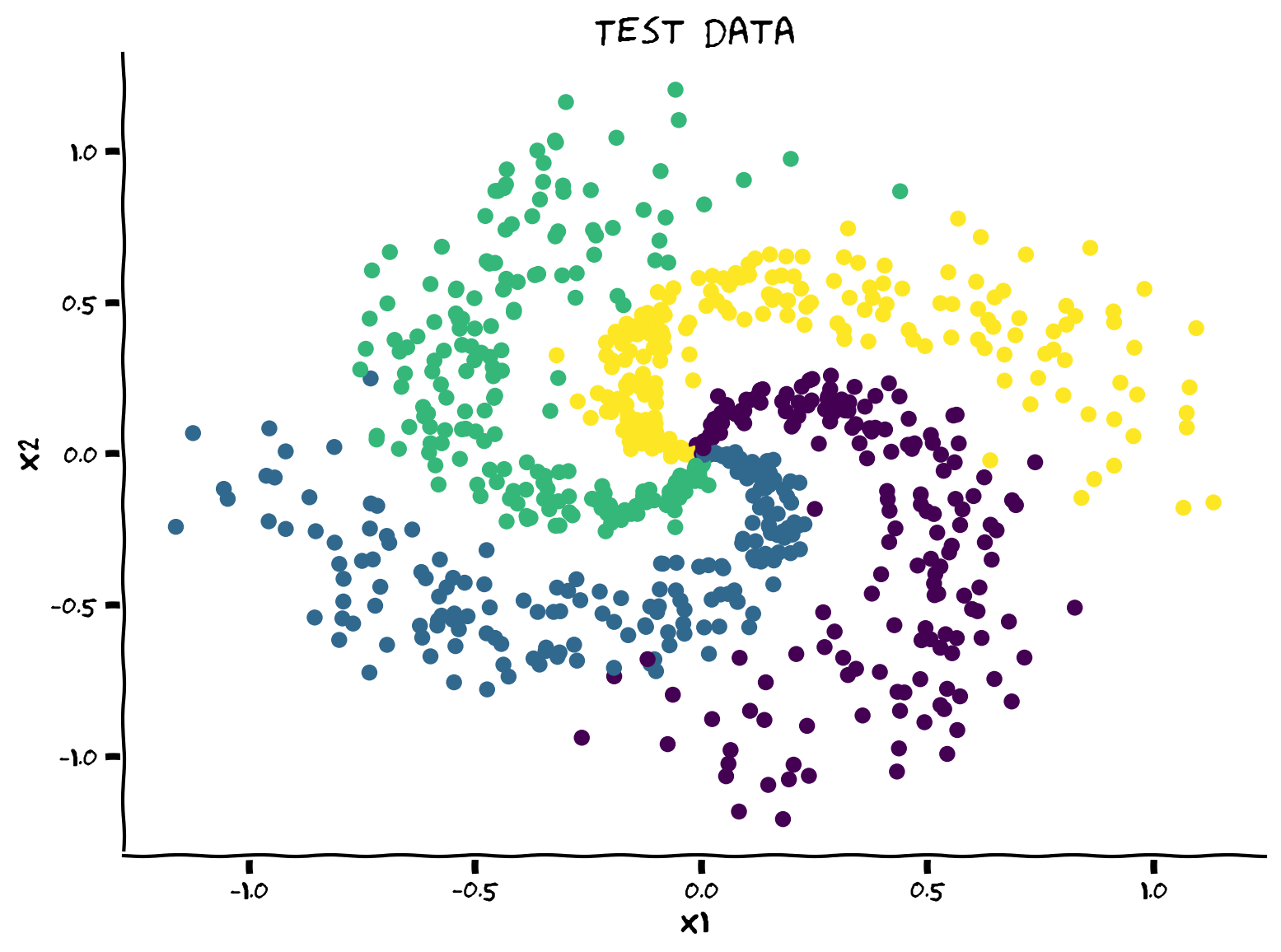
スパイラルデータセットと損失関数が揃ったので、今度はシンプルな訓練/テスト分割を実装して、トレーニングと検証を行いましょう。

手順:

データセットのシャッフル
訓練/テスト分割（テストに20%）
データローダーの定義
トレーニングと評価

def shuffle_and_split_data(X, y, seed):
  """
  Helper function to shuffle and split incoming data

  Args:
    X: torch.tensor
      Input data
    y: torch.tensor
      Corresponding target variables
    seed: int
      Set seed for reproducibility

  Returns:
    X_test: torch.tensor
      Test data [20% of X]
    y_test: torch.tensor
      Labels corresponding to above mentioned test data
    X_train: torch.tensor
      Train data [80% of X]
    y_train: torch.tensor
      Labels corresponding to above mentioned train data
  """
  torch.manual_seed(seed)
  # Number of samples
  N = X.shape[0]
  ####################################################################
  # Fill in missing code below (...),
  # then remove or comment the line below to test your function
  raise NotImplementedError("Shuffle & split data")
  ####################################################################
  # Shuffle data
  shuffled_indices = ...   # Get indices to shuffle data, could use torch.randperm
  X = X[shuffled_indices]
  y = y[shuffled_indices]

  # Split data into train/test
  test_size = ...    # Assign test datset size using 20% of samples
  X_test = X[:test_size]
  y_test = y[:test_size]
  X_train = X[test_size:]
  y_train = y[test_size:]

  return X_test, y_test, X_train, y_train



## Uncomment below to test your function
# X_test, y_test, X_train, y_train = shuffle_and_split_data(X, y, seed=SEED)
# plt.figure()
# plt.scatter(X_test[:, 0], X_test[:, 1], c=y_test)
# plt.xlabel('x1')
# plt.ylabel('x2')
# plt.title('Test data')
# plt.show()

解答を見る$

出力例:

# @title Submit your feedback
content_review(f"{feedback_prefix}_Implement_it_for_a_classification_task_Exercise")

そしてこれをPyTorchのデータローダーに変換する必要があります。PyTorchでのデータ読み込みは2つの部分に分かれます:

データはDataset親クラスでラップされ、getitem と len メソッドをオーバーライドする必要があります。この時点ではデータはメモリにロードされていません。PyTorchは必要な分だけメモリにロードします。ここでは TensorDataset がこれを直接行います。
実際にバッチ単位でデータを読み込みメモリに置くDataloaderを使用します。また、num_workers > 0 のオプションはマルチスレッドを可能にし、複数のバッチをキューに準備して高速化します。

g_seed = torch.Generator()
g_seed.manual_seed(SEED)

batch_size = 128
test_data = TensorDataset(X_test, y_test)
test_loader = DataLoader(test_data, batch_size=batch_size,
                         shuffle=False, num_workers=2,
                         worker_init_fn=seed_worker,
                         generator=g_seed)

train_data = TensorDataset(X_train, y_train)
train_loader = DataLoader(train_data, batch_size=batch_size, drop_last=True,
                          shuffle=True, num_workers=2,
                          worker_init_fn=seed_worker,
                          generator=g_seed)

汎用的なトレーニングと評価のコードを書いて、次回のチュートリアルでも使えるようにしましょう。何をしているかを理解するために必ず復習してください。

model.train() はモデルがトレーニングモードであることを示します。ドロップアウトやバッチ正規化など、トレーニング時とテスト時で挙動が異なる層が適切に動作できるようにします。トレーニングモードをオフにするには model.eval() を使います。

def train_test_classification(net, criterion, optimizer, train_loader,
                              test_loader, num_epochs=1, verbose=True,
                              training_plot=False, device='cpu'):
  """
  Accumulate training loss/Evaluate performance

  Args:
    net: instance of Net class
      Describes the model with ReLU activation, batch size 128
    criterion: torch.nn type
      Criterion combines LogSoftmax and NLLLoss in one single class.
    optimizer: torch.optim type
      Implements Adam algorithm.
    train_loader: torch.utils.data type
      Combines the train dataset and sampler, and provides an iterable over the given dataset.
    test_loader: torch.utils.data type
      Combines the test dataset and sampler, and provides an iterable over the given dataset.
    num_epochs: int
      Number of epochs [default: 1]
    verbose: boolean
      If True, print statistics
    training_plot=False
      If True, display training plot
    device: string
      CUDA/GPU if available, CPU otherwise

  Returns:
    Nothing
  """
  net.train()
  training_losses = []
  for epoch in tqdm(range(num_epochs)):  # Loop over the dataset multiple times
    running_loss = 0.0
    for i, data in enumerate(train_loader, 0):
      # Get the inputs; data is a list of [inputs, labels]
      inputs, labels = data
      inputs = inputs.to(device).float()
      labels = labels.to(device).long()

      # Zero the parameter gradients
      optimizer.zero_grad()

      # forward + backward + optimize
      outputs = net(inputs)

      loss = criterion(outputs, labels)
      loss.backward()
      optimizer.step()

      # Print statistics
      if verbose:
        training_losses += [loss.item()]

  net.eval()

  def test(data_loader):
    """
    Function to gauge network performance

    Args:
      data_loader: torch.utils.data type
      Combines the test dataset and sampler, and provides an iterable over the given dataset.

    Returns:
      acc: float
        Performance of the network
      total: int
        Number of datapoints in the dataloader
    """
    correct = 0
    total = 0
    for data in data_loader:
      inputs, labels = data
      inputs = inputs.to(device).float()
      labels = labels.to(device).long()

      outputs = net(inputs)
      _, predicted = torch.max(outputs, 1)
      total += labels.size(0)
      correct += (predicted == labels).sum().item()

    acc = 100 * correct / total
    return total, acc

  train_total, train_acc = test(train_loader)
  test_total, test_acc = test(test_loader)

  if verbose:
    print(f"Accuracy on the {train_total} training samples: {train_acc:0.2f}")
    print(f"Accuracy on the {test_total} testing samples: {test_acc:0.2f}")

  if training_plot:
    plt.plot(training_losses)
    plt.xlabel('Batch')
    plt.ylabel('Training loss')
    plt.show()

  return train_acc, test_acc

考えてみよう！ 2.3.1: `.eval()` と `.train()` の意味は？

MLPモデルに対して net.train() と net.eval() を使う必要はありますか？なぜですか？

解答を見る$

# @title Submit your feedback
content_review(f"{feedback_prefix}_Whats_the_point_of_eval()_and_train()_Discussion")

では、すべてをまとめて、あなたの最初のやや深いモデルをトレーニングしましょう！

set_seed(SEED)
net = Net('ReLU()', X_train.shape[1], [128], K).to(DEVICE)
criterion = nn.CrossEntropyLoss()
optimizer = optim.Adam(net.parameters(), lr=1e-3)
num_epochs = 100

_, _ = train_test_classification(net, criterion, optimizer, train_loader,
                                 test_loader, num_epochs=num_epochs,
                                 training_plot=True, device=DEVICE)

最後に、学習した決定マップを可視化しましょう。時間がないと思うので、コードを書くのは今回は省略します！しかし、次回は別の可視化手法から始めるので、必ず復習しておいてください。

def sample_grid(M=500, x_max=2.0):
  """
  Helper function to simulate sample meshgrid

  Args:
    M: int
      Size of the constructed tensor with meshgrid
    x_max: float
      Defines range for the set of points

  Returns:
    X_all: torch.tensor
      Concatenated meshgrid tensor
  """
  ii, jj = torch.meshgrid(torch.linspace(-x_max, x_max, M),
                          torch.linspace(-x_max, x_max, M),
                          indexing="ij")
  X_all = torch.cat([ii.unsqueeze(-1),
                     jj.unsqueeze(-1)],
                     dim=-1).view(-1, 2)
  return X_all


def plot_decision_map(X_all, y_pred, X_test, y_test,
                      M=500, x_max=2.0, eps=1e-3):
  """
  Helper function to plot decision map

  Args:
    X_all: torch.tensor
      Concatenated meshgrid tensor
    y_pred: torch.tensor
      Labels predicted by the network
    X_test: torch.tensor
      Test data
    y_test: torch.tensor
      Labels of the test data
    M: int
      Size of the constructed tensor with meshgrid
    x_max: float
      Defines range for the set of points
    eps: float
      Decision threshold

  Returns:
    Nothing
  """
  decision_map = torch.argmax(y_pred, dim=1)

  for i in range(len(X_test)):
    indices = (X_all[:, 0] - X_test[i, 0])**2 + (X_all[:, 1] - X_test[i, 1])**2 < eps
    decision_map[indices] = (K + y_test[i]).long()

  decision_map = decision_map.view(M, M)
  plt.imshow(decision_map, extent=[-x_max, x_max, -x_max, x_max], cmap='jet')
  plt.xlabel('x1')
  plt.ylabel('x2')
  plt.show()

X_all = sample_grid()
y_pred = net(X_all.to(DEVICE)).cpu()
plot_decision_map(X_all, y_pred, X_test, y_test)

考えてみよう！ 2.3.2: 一般化できている？

このモデルは訓練分布外でもうまく機能していると思いますか？なぜですか？

解答を見る$

モデルの一般化能力を高めるためにどんな提案をしますか？考えてみて、ポッドで議論してください。

解答を見る$

# @title Submit your feedback
content_review(f"{feedback_prefix}_Does_it_generalize_well_Discussion")

まとめ

このチュートリアルでは、多層パーセプトロン（MLP）について探求しました。特に、人工ニューラルネットワークと生物学的ニューラルネットワークの類似点（詳細はボーナスセクション参照）について議論し、普遍近似定理を学び、PyTorchでMLPを実装しました。

ボーナス: ニューロンの生理学とディープラーニングへの動機付け

このセクションでは、ニューロンの生物物理学から出発し、一連の近似を経てReLU非線形性を導出することで、ディープラーニングで最も人気のある非線形関数の一つであるReLUの動機付けを行います。また、ニューロンの生物物理学が脳内の信号伝達速度の時間スケールを設定していることを示します。この時間スケールは、脳の高速な知覚・運動処理を支える神経回路が過度に深くない可能性を示唆しています。

# @title Video 5: Biological to Artificial Neurons
from ipywidgets import widgets
from IPython.display import YouTubeVideo
from IPython.display import IFrame
from IPython.display import display


class PlayVideo(IFrame):
  def __init__(self, id, source, page=1, width=400, height=300, **kwargs):
    self.id = id
    if source == 'Bilibili':
      src = f'https://player.bilibili.com/player.html?bvid={id}&page={page}'
    elif source == 'Osf':
      src = f'https://mfr.ca-1.osf.io/render?url=https://osf.io/download/{id}/?direct%26mode=render'
    super(PlayVideo, self).__init__(src, width, height, **kwargs)


def display_videos(video_ids, W=400, H=300, fs=1):
  tab_contents = []
  for i, video_id in enumerate(video_ids):
    out = widgets.Output()
    with out:
      if video_ids[i][0] == 'Youtube':
        video = YouTubeVideo(id=video_ids[i][1], width=W,
                             height=H, fs=fs, rel=0)
        print(f'Video available at https://youtube.com/watch?v={video.id}')
      else:
        video = PlayVideo(id=video_ids[i][1], source=video_ids[i][0], width=W,
                          height=H, fs=fs, autoplay=False)
        if video_ids[i][0] == 'Bilibili':
          print(f'Video available at https://www.bilibili.com/video/{video.id}')
        elif video_ids[i][0] == 'Osf':
          print(f'Video available at https://osf.io/{video.id}')
      display(video)
    tab_contents.append(out)
  return tab_contents


video_ids = [('Youtube', 'ELAbflymSLo'), ('Bilibili', 'BV1mf4y157vf')]
tab_contents = display_videos(video_ids, W=854, H=480)
tabs = widgets.Tab()
tabs.children = tab_contents
for i in range(len(tab_contents)):
  tabs.set_title(i, video_ids[i][0])
display(tabs)

# @title Submit your feedback
content_review(f"{feedback_prefix}_Biological_to_Artificial_Neurons_Bonus_Video")

漏れ積分発火（LIF）ニューロンモデル

LIFニューロンの基本的なアイデアは、ニューロンの電気生理学が理解されるずっと前の1907年にLouis Édouard Lapicqueによって提案されました（Lapicqueの論文翻訳を参照）。モデルの詳細はPeter DayanとLaurence F. Abbottの著書Theoretical neuroscienceにあります。

モデルの動力学は以下の式で定義されます。

\frac{d V_m}{d t}=\left\{\begin{array}{cc} \frac{1}{C_m}\left(-\frac{V_m}{R_m} + I \right) & t>t_{rest} \\ 0 & \text { otherwise } \end{array}\right.

ここで $V_{m}$ 、 $C_{m}$ 、 $R_{m}$ はそれぞれ膜電位、容量、抵抗を表し、 $-\frac{V_{m}}{R_{m}}$ は漏れ電流を示します。入力電流 $I$ が十分強く $V_{m}$ が閾値 $V_{\rm th}$ に達すると、一瞬スパイクを発し、その後 $V_{m}$ は $V_{\rm reset} < V_{\rm th}$ にリセットされ、 $\tau_{\rm ref}$ ミリ秒間 $V_{\rm reset}$ に留まります。これは活動電位中の不応期を模倣しています（講義では $V_{\rm reset}$ と $\tau_{\rm ref}$ はゼロと仮定しています）。

\begin{eqnarray}
$V_{m}(t)=V_{$ $\rm reset} \text{ for } t\in(t_{\text{sp}}, t_{\text{sp}} + \tau_{\text{ref}}$ ]
\end{eqnarray}

ここで $t_{\rm sp}$ は $V_{m}(t)$ が $V_{\rm th}$ を超えたスパイク時刻です。

このようにLIFモデルはニューロンが以下の特徴を持つことを捉えています:

シナプス入力の空間的・時間的統合を行う
電位が閾値に達するとスパイクを発生させる
活動電位中は不応期になる
漏れ膜を持つ

ニューロンの計算モデルの詳細はNMAのBiological Neuron Modelsチュートリアル1を参照してください。特にNMA-CN 2021ではこのTutorial$を参照してください。

LIFニューロンのシミュレーション

以下のセルにはLIFニューロンモデルの関数があり、引数の説明も記載されています。

オイラー法を使って微分の数値近似を行うため、モデルの動力学は以下のように実装します。

V_m^{[n]}=\left\{\begin{array}{cc} V_m^{[n-1]} + \frac{1}{C_m}\left(-\frac{V_m^{[n-1]}}{R_m}+I \right) \Delta t & t>t_{r e s t} \\ 0 & \text { otherwise } \end{array}\right.

ここで上付き添字 $[\cdot]$ は時刻点を示します。

def run_LIF(I, T=50, dt=0.1, tau_ref=10,
            Rm=1, Cm=10, Vth=1, V_spike=0.5):
  """
  Simulate the LIF dynamics with external input current

  Args:
    I          : int
      Input current (mA)
    T          : int
      Total time to simulate (msec)
    dt         : float
      Simulation of time step (msec)
    tau_ref    : int
      Refractory period (msec)
    Rm         : int
      Resistance (kOhm)
    Cm         : int
      Capacitance (uF)
    Vth        : int
      Spike threshold (V)
    V_spike    : float
      Spike delta (V)

  Returns:
    time       : list
      Time points
    Vm         : list
      Tracking membrane potentials
  """

  # Set up array of time steps
  time = torch.arange(0, T + dt, dt)

  # Set up array for tracking Vm
  Vm = torch.zeros(len(time))

  # Iterate over each time step
  t_rest = 0
  for i, t in enumerate(time):

    # If t is after refractory period
    if t > t_rest:
      Vm[i] = Vm[i-1] + 1/Cm*(-Vm[i-1]/Rm + I)  * dt

    # If Vm is over the threshold
    if Vm[i] >= Vth:

      # Increase volatage by change due to spike
      Vm[i] += V_spike

      # Set up new refactory period
      t_rest = t + tau_ref

  return time, Vm


sim_time, Vm = run_LIF(1.5)
# Plot the membrane voltage across time
plt.plot(sim_time, Vm)
plt.title('LIF Neuron Output')
plt.ylabel('Membrane Potential (V)')
plt.xlabel('Time (msec)')
plt.show()

インタラクティブデモ: 異なる $R_m$ と $\tau_{ref}$ によるニューロンの伝達関数探索

実際のニューロンはスパイク数を変化させて情報を伝達します。つまり、入力電流が大きいほどスパイク頻度が上がります。そこで、入力電流に対するスパイク数の関数としてニューロンの入出力伝達関数を特徴づけるのが理にかなっています。ニューロンの伝達関数をプロットし、膜抵抗と不応期によってどのように変化するか見てみましょう。

# @title

# @markdown Make sure you execute this cell to enable the widget!
my_layout = widgets.Layout()

@widgets.interact(Rm=widgets.FloatSlider(1., min=1, max=100.,
                                         step=0.1, layout=my_layout),
                  tau_ref=widgets.FloatSlider(1., min=1, max=100.,
                                            step=0.1, layout=my_layout)
                  )


def plot_IF_curve(Rm, tau_ref):
  """
  Helper function to plot frequency-current curve

  Args:
    Rm         : int
      Resistance (kOhm)
    tau_ref    : int
      Refractory period (msec)

  Returns:
    Nothing
  """
  T = 1000  # Total time to simulate (msec)
  dt = 1  # Simulation time step (msec)
  Vth = 1  # Spike threshold (V)
  Is_max = 2
  Is = torch.linspace(0, Is_max, 10)
  spike_counts = []
  for I in Is:
    _, Vm = run_LIF(I, T=T, dt=dt, Vth=Vth, Rm=Rm, tau_ref=tau_ref)
    spike_counts += [torch.sum(Vm > Vth)]

  plt.plot(Is, spike_counts)
  plt.title('LIF Neuron: Transfer Function')
  plt.ylabel('Spike count')
  plt.xlabel('I (mA)')
  plt.xlim(0, Is_max)
  plt.ylim(0, 80)
  plt.show()

考えてみよう！: 実際のニューロンと人工ニューロンの類似点

膜抵抗 ( $R_m$ ) が無限大で不応期 ( $\tau_{ref}$ ) が小さい場合、何が起こるでしょうか？なぜでしょう？

10分間かけて、ポッドで実際のニューロンと人工ニューロンの類似点について議論してください。

解答を見る$

# @title Submit your feedback
content_review(f"{feedback_prefix}_Real_and_Artificial_neuron_similarities_Bonus_Discussion")

チュートリアル 1: 生物学的ニューラルネットワーク vs. 人工ニューラルネットワーク

チュートリアルの目的

セットアップ

セクション0: MLPの紹介

セクション1: MLPが必要な理由

コーディング演習1: ReLUを用いた関数近似

セクション2: PyTorchにおけるMLP

コーディング演習 2: Pytorchで汎用的なMLPを実装する

セクション 2.1: MLPによる分類

コーディング演習 2.1: バッチクロスエントロピー損失の実装

セクション 2.2: スパイラル分類データセット

セクション 2.3: トレーニングと評価

コーディング演習 2.3: 分類タスクの実装

考えてみよう！ 2.3.1: .eval() と .train() の意味は？

考えてみよう！ 2.3.2: 一般化できている？

まとめ

ボーナス: ニューロンの生理学とディープラーニングへの動機付け

漏れ積分発火（LIF）ニューロンモデル

LIFニューロンのシミュレーション

インタラクティブデモ: 異なる RmR_mRm​ と τref\tau_{ref}τref​ によるニューロンの伝達関数探索

考えてみよう！: 実際のニューロンと人工ニューロンの類似点

考えてみよう！ 2.3.1: `.eval()` と `.train()` の意味は？

インタラクティブデモ: 異なる $R_m$ と $\tau_{ref}$ によるニューロンの伝達関数探索