チュートリアル 3: 深層線形ニューラルネットワーク

第1週、第2日目：線形ディープラーニング

Neuromatch Academyによる

コンテンツ作成者: Saeed Salehi, Spiros Chavlis, Andrew Saxe

コンテンツレビュアー: Polina Turishcheva, Antoine De Comite

コンテンツ編集者: Anoop Kulkarni

制作編集者: Khalid Almubarak, Gagana B, Spiros Chavlis

チュートリアルの目的

深層線形ニューラルネットワーク
学習ダイナミクスと特異値分解
表現類似性解析
幻想的相関と倫理

# @title Tutorial slides
from IPython.display import IFrame
link_id = "bncr8"
print(f"If you want to download the slides: https://osf.io/download/{link_id}/")
IFrame(src=f"https://mfr.ca-1.osf.io/render?url=https://osf.io/{link_id}/?direct%26mode=render%26action=download%26mode=render", width=854, height=480)

セットアップ

このチュートリアルはGPU不要です！

# @title Install and import feedback gadget


from vibecheck import DatatopsContentReviewContainer
def content_review(notebook_section: str):
    return DatatopsContentReviewContainer(
        "",  # No text prompt
        notebook_section,
        {
            "url": "https://pmyvdlilci.execute-api.us-east-1.amazonaws.com/klab",
            "name": "neuromatch_dl",
            "user_key": "f379rz8y",
        },
    ).render()


feedback_prefix = "W1D2_T3"

# Imports
import math
import torch
import matplotlib

import numpy as np
import matplotlib.pyplot as plt

import torch.nn as nn
import torch.optim as optim

# @title Figure settings
import logging
logging.getLogger('matplotlib.font_manager').disabled = True

from matplotlib import gridspec
from ipywidgets import interact, IntSlider, FloatSlider, fixed
from ipywidgets import FloatLogSlider, Layout, VBox
from ipywidgets import interactive_output
from mpl_toolkits.axes_grid1 import make_axes_locatable

import warnings
warnings.filterwarnings("ignore")

%config InlineBackend.figure_format = 'retina'
plt.style.use("https://raw.githubusercontent.com/NeuromatchAcademy/content-creation/main/nma.mplstyle")

# @title Plotting functions

def plot_x_y_hier_data(im1, im2, subplot_ratio=[1, 2]):
  """
  Plot hierarchical data of labels vs features
  for all samples

  Args:
    im1: np.ndarray
      Input Dataset
    im2: np.ndarray
      Targets
    subplot_ratio: list
      Subplot ratios used to create subplots of varying sizes

  Returns:
    Nothing
  """
  fig = plt.figure(figsize=(12, 5))
  gs = gridspec.GridSpec(1, 2, width_ratios=subplot_ratio)
  ax0 = plt.subplot(gs[0])
  ax1 = plt.subplot(gs[1])
  ax0.imshow(im1, cmap="cool")
  ax1.imshow(im2, cmap="cool")
  ax0.set_title("Labels of all samples")
  ax1.set_title("Features of all samples")
  ax0.set_axis_off()
  ax1.set_axis_off()
  plt.tight_layout()
  plt.show()


def plot_x_y_hier_one(im1, im2, subplot_ratio=[1, 2]):
  """
  Plot hierarchical data of labels vs features
  for a single sample

  Args:
    im1: np.ndarray
      Input Dataset
    im2: np.ndarray
      Targets
    subplot_ratio: list
      Subplot ratios used to create subplots of varying sizes

  Returns:
    Nothing
  """
  fig = plt.figure(figsize=(12, 1))
  gs = gridspec.GridSpec(1, 2, width_ratios=subplot_ratio)
  ax0 = plt.subplot(gs[0])
  ax1 = plt.subplot(gs[1])
  ax0.imshow(im1, cmap="cool")
  ax1.imshow(im2, cmap="cool")
  ax0.set_title("Labels of a single sample")
  ax1.set_title("Features of a single sample")
  ax0.set_axis_off()
  ax1.set_axis_off()
  plt.tight_layout()
  plt.show()


def plot_tree_data(label_list = None, feature_array = None, new_feature = None):
  """
  Plot tree data

  Args:
    label_list: np.ndarray
      List of labels [default: None]
    feature_array: np.ndarray
      List of features [default: None]
    new_feature: string
      Enables addition of new features

  Returns:
    Nothing
  """
  cmap = matplotlib.colors.ListedColormap(['cyan', 'magenta'])
  n_features = 10
  n_labels = 8
  im1 = np.eye(n_labels)
  if feature_array is None:
    im2 = np.array([[1, 1, 1, 1, 1, 1, 1, 1],
                      [0, 0, 0, 0, 0, 0, 0, 0],
                      [0, 0, 0, 0, 1, 1, 1, 1],
                      [1, 1, 1, 1, 0, 0, 0, 0],
                      [0, 0, 0, 0, 0, 0, 1, 1],
                      [0, 0, 1, 1, 0, 0, 0, 0],
                      [1, 1, 0, 0, 0, 0, 0, 0],
                      [0, 0, 0, 0, 1, 1, 0, 0],
                      [0, 1, 1, 1, 0, 0, 0, 0],
                      [0, 0, 0, 0, 1, 1, 0, 1]]).T
    im2[im2 == 0] = -1
    feature_list = ['can_grow',
                    'is_mammal',
                    'has_leaves',
                    'can_move',
                    'has_trunk',
                    'can_fly',
                    'can_swim',
                    'has_stem',
                    'is_warmblooded',
                    'can_flower']
  else:
    im2 = feature_array
  if label_list is None:
    label_list = ['Goldfish', 'Tuna', 'Robin', 'Canary',
                  'Rose', 'Daisy', 'Pine', 'Oak']
  fig = plt.figure(figsize=(12, 7))
  gs = gridspec.GridSpec(1, 2, width_ratios=[1, 1.35])
  ax1 = plt.subplot(gs[0])
  ax2 = plt.subplot(gs[1])
  ax1.imshow(im1, cmap=cmap)
  if feature_array is None:
    implt = ax2.imshow(im2, cmap=cmap, vmin=-1.0, vmax=1.0)
  else:
    implt = ax2.imshow(im2[:, -n_features:], cmap=cmap, vmin=-1.0, vmax=1.0)
  divider = make_axes_locatable(ax2)
  cax = divider.append_axes("right", size="5%", pad=0.1)
  cbar = plt.colorbar(implt, cax=cax, ticks=[-0.5, 0.5])
  cbar.ax.set_yticklabels(['no', 'yes'])
  ax1.set_title("Labels")
  ax1.set_yticks(ticks=np.arange(n_labels))
  ax1.set_yticklabels(labels=label_list)
  ax1.set_xticks(ticks=np.arange(n_labels))
  ax1.set_xticklabels(labels=label_list, rotation='vertical')
  ax2.set_title("{} random Features".format(n_features))
  ax2.set_yticks(ticks=np.arange(n_labels))
  ax2.set_yticklabels(labels=label_list)
  if feature_array is None:
    ax2.set_xticks(ticks=np.arange(n_features))
    ax2.set_xticklabels(labels=feature_list, rotation='vertical')
  else:
    ax2.set_xticks(ticks=[n_features-1])
    ax2.set_xticklabels(labels=[new_feature], rotation='vertical')
  plt.tight_layout()
  plt.show()


def plot_loss(loss_array,
              title="Training loss (Mean Squared Error)",
              c="r"):
  """
  Plot loss function

  Args:
    c: string
      Specifies plot color
    title: string
      Specifies plot title
    loss_array: np.ndarray
      Log of MSE loss per epoch

  Returns:
    Nothing
  """
  plt.figure(figsize=(10, 5))
  plt.plot(loss_array, color=c)
  plt.xlabel("Epoch")
  plt.ylabel("MSE")
  plt.title(title)
  plt.show()


def plot_loss_sv(loss_array, sv_array):
  """
  Plot loss function

  Args:
    sv_array: np.ndarray
      Log of singular values/modes across epochs
    loss_array: np.ndarray
      Log of MSE loss per epoch

  Returns:
    Nothing
  """
  n_sing_values = sv_array.shape[1]
  sv_array = sv_array / np.max(sv_array)
  cmap = plt.cm.get_cmap("Set1", n_sing_values)

  _, (plot1, plot2) = plt.subplots(2, 1, sharex=True, figsize=(10, 10))
  plot1.set_title("Training loss (Mean Squared Error)")
  plot1.plot(loss_array, color='r')

  plot2.set_title("Evolution of singular values (modes)")
  for i in range(n_sing_values):
    plot2.plot(sv_array[:, i], c=cmap(i))
  plot2.set_xlabel("Epoch")
  plt.show()


def plot_loss_sv_twin(loss_array, sv_array):
  """
  Plot learning dynamics

  Args:
    sv_array: np.ndarray
      Log of singular values/modes across epochs
    loss_array: np.ndarray
      Log of MSE loss per epoch

  Returns:
    Nothing
  """
  n_sing_values = sv_array.shape[1]
  sv_array = sv_array / np.max(sv_array)
  cmap = plt.cm.get_cmap("winter", n_sing_values)

  fig = plt.figure(figsize=(10, 5))
  ax1 = plt.gca()
  ax1.set_title("Learning Dynamics")
  ax1.set_xlabel("Epoch")
  ax1.set_ylabel("Mean Squared Error", c='r')
  ax1.tick_params(axis='y', labelcolor='r')
  ax1.plot(loss_array, color='r')

  ax2 = ax1.twinx()
  ax2.set_ylabel("Singular values (modes)", c='b')
  ax2.tick_params(axis='y', labelcolor='b')
  for i in range(n_sing_values):
    ax2.plot(sv_array[:, i], c=cmap(i))

  fig.tight_layout()
  plt.show()


def plot_ills_sv_twin(ill_array, sv_array, ill_label):
  """
  Plot network training evolution
  and illusory correlations

  Args:
    sv_array: np.ndarray
      Log of singular values/modes across epochs
    ill_array: np.ndarray
      Log of illusory correlations per epoch
    ill_label: np.ndarray
      Log of labels associated with illusory correlations

  Returns:
    Nothing
  """
  n_sing_values = sv_array.shape[1]
  sv_array = sv_array / np.max(sv_array)
  cmap = plt.cm.get_cmap("winter", n_sing_values)

  fig = plt.figure(figsize=(10, 5))
  ax1 = plt.gca()
  ax1.set_title("Network training and the Illusory Correlations")
  ax1.set_xlabel("Epoch")
  ax1.set_ylabel(ill_label, c='r')
  ax1.tick_params(axis='y', labelcolor='r')
  ax1.plot(ill_array, color='r', linewidth=3)
  ax1.set_ylim(-1.05, 1.05)

  ax2 = ax1.twinx()
  ax2.set_ylabel("Singular values (modes)", c='b')
  ax2.tick_params(axis='y', labelcolor='b')
  for i in range(n_sing_values):
    ax2.plot(sv_array[:, i], c=cmap(i))

  fig.tight_layout()
  plt.show()


def plot_loss_sv_rsm(loss_array, sv_array, rsm_array, i_ep):
  """
  Plot learning dynamics

  Args:
    sv_array: np.ndarray
      Log of singular values/modes across epochs
    loss_array: np.ndarray
      Log of MSE loss per epoch
    rsm_array: torch.tensor
      Representation similarity matrix
    i_ep: int
      Which epoch to show

  Returns:
    Nothing
  """
  n_ep = loss_array.shape[0]
  rsm_array = rsm_array / np.max(rsm_array)
  sv_array = sv_array / np.max(sv_array)

  n_sing_values = sv_array.shape[1]
  cmap = plt.cm.get_cmap("winter", n_sing_values)

  fig = plt.figure(figsize=(14, 5))
  gs = gridspec.GridSpec(1, 2, width_ratios=[5, 3])

  ax0 = plt.subplot(gs[1])
  ax0.yaxis.tick_right()
  implot = ax0.imshow(rsm_array[i_ep], cmap="Purples", vmin=0.0, vmax=1.0)
  divider = make_axes_locatable(ax0)
  cax = divider.append_axes("right", size="5%", pad=0.9)
  cbar = plt.colorbar(implot, cax=cax, ticks=[])
  cbar.ax.set_ylabel('Similarity', fontsize=12)
  ax0.set_title("RSM at epoch {}".format(i_ep), fontsize=16)
  ax0.set_yticks(ticks=np.arange(n_sing_values))
  ax0.set_yticklabels(labels=item_names)
  ax0.set_xticks(ticks=np.arange(n_sing_values))
  ax0.set_xticklabels(labels=item_names, rotation='vertical')

  ax1 = plt.subplot(gs[0])
  ax1.set_title("Learning Dynamics", fontsize=16)
  ax1.set_xlabel("Epoch")
  ax1.set_ylabel("Mean Squared Error", c='r')
  ax1.tick_params(axis='y', labelcolor='r', direction="in")
  ax1.plot(np.arange(n_ep), loss_array, color='r')
  ax1.axvspan(i_ep-2, i_ep+2, alpha=0.2, color='m')

  ax2 = ax1.twinx()
  ax2.set_ylabel("Singular values", c='b')
  ax2.tick_params(axis='y', labelcolor='b', direction="in")
  for i in range(n_sing_values):
    ax2.plot(np.arange(n_ep), sv_array[:, i], c=cmap(i))
  ax1.set_xlim(-1, n_ep+1)
  ax2.set_xlim(-1, n_ep+1)

  plt.show()

# @title Helper functions

def build_tree(n_levels, n_branches, probability,
               to_np_array=True):
  """
  Builds tree

  Args:
    n_levels: int
      Number of levels in tree
    n_branches: int
      Number of branches in tree
    probability: float
      Flipping probability
    to_np_array: boolean
      If true, represent tree as np.ndarray

  Returns:
    tree: dict if to_np_array=False
          np.ndarray otherwise
      Tree
  """
  assert 0.0 <= probability <= 1.0

  tree = {}

  tree["level"] = [0]
  for i in range(1, n_levels+1):
    tree["level"].extend([i]*(n_branches**i))

  tree["pflip"] = [probability]*len(tree["level"])

  tree["parent"] = [None]
  k = len(tree["level"])-1
  for j in range(k//n_branches):
    tree["parent"].extend([j]*n_branches)

  if to_np_array:
    tree["level"] = np.array(tree["level"])
    tree["pflip"] = np.array(tree["pflip"])
    tree["parent"] = np.array(tree["parent"])

  return tree


def sample_from_tree(tree, n):
  """
  Generates n samples from a tree

  Args:
    tree: np.ndarray/dictionary
      Tree
    n: int
      Number of levels in tree

  Returns:
    x: np.ndarray
      Sample from tree
  """
  items = [i for i, v in enumerate(tree["level"]) if v == max(tree["level"])]
  n_items = len(items)
  x = np.zeros(shape=(n, n_items))
  rand_temp = np.random.rand(n, len(tree["pflip"]))
  flip_temp = np.repeat(tree["pflip"].reshape(1, -1), n, 0)
  samp = (rand_temp > flip_temp) * 2 - 1

  for i in range(n_items):
    j = items[i]
    prop = samp[:, j]
    while tree["parent"][j] is not None:
      j = tree["parent"][j]
      prop = prop * samp[:, j]
    x[:, i] = prop.T
  return x


def generate_hsd():
  """
  Building the tree

  Args:
    None

  Returns:
    tree_labels: np.ndarray
      Tree Labels
    tree_features: np.ndarray
      Sample from tree
  """
  n_branches = 2  # 2 branches at each node
  probability = .15  # flipping probability
  n_levels = 3  # number of levels (depth of tree)
  tree = build_tree(n_levels, n_branches, probability, to_np_array=True)
  tree["pflip"][0] = 0.5
  n_samples = 10000 # Sample this many features

  tree_labels = np.eye(n_branches**n_levels)
  tree_features = sample_from_tree(tree, n_samples).T
  return tree_labels, tree_features


def linear_regression(X, Y):
  """
  Analytical Linear regression

  Args:
    X: np.ndarray
      Input features
    Y: np.ndarray
      Targets

  Returns:
    W: np.ndarray
      Analytical solution
      W = Y @ X.T @ np.linalg.inv(X @ X.T)
  """
  assert isinstance(X, np.ndarray)
  assert isinstance(Y, np.ndarray)
  M, Dx = X.shape
  N, Dy = Y.shape
  assert Dx == Dy
  W = Y @ X.T @ np.linalg.inv(X @ X.T)
  return W


def add_feature(existing_features, new_feature):
  """
  Adding new features to existing tree

  Args:
    existing_features: np.ndarray
      List of features already present in the tree
    new_feature: list
      List of new features to be added

  Returns:
    New features augmented with existing features
  """
  assert isinstance(existing_features, np.ndarray)
  assert isinstance(new_feature, list)
  new_feature = np.array([new_feature]).T
  return np.hstack((tree_features, new_feature))


def net_svd(model, in_dim):
  """
  Performs a Singular Value Decomposition on
  given model weights

  Args:
    model: torch.nn.Module
      Neural network model
    in_dim: int
      The input dimension of the model

  Returns:
    U: torch.tensor
      Orthogonal Matrix
    Σ: torch.tensor
      Diagonal Matrix
    V: torch.tensor
      Orthogonal Matrix
  """
  W_tot = torch.eye(in_dim)
  for weight in model.parameters():
    W_tot = weight.detach() @ W_tot
  U, SIGMA, V = torch.svd(W_tot)
  return U, SIGMA, V


def net_rsm(h):
  """
  Calculates the Representational Similarity Matrix

  Args:
    h: torch.Tensor
      Activity of a hidden layer

  Returns:
    rsm: torch.Tensor
      Representational Similarity Matrix
  """
  rsm = h @ h.T
  return rsm


def initializer_(model, gamma=1e-12):
  """
  In-place Re-initialization of weights

  Args:
    model: torch.nn.Module
      PyTorch neural net model
    gamma: float
      Initialization scale

  Returns:
    Nothing
  """
  for weight in model.parameters():
    n_out, n_in = weight.shape
    sigma = gamma / math.sqrt(n_in + n_out)
    nn.init.normal_(weight, mean=0.0, std=sigma)


def test_initializer_ex(seed):
  """
  Testing initializer implementation

  Args:
    seed: int
      Set for reproducibility

  Returns:
    Nothing
  """
  torch.manual_seed(seed)
  model = LNNet(5000, 5000, 1)
  try:
    ex_initializer_(model, gamma=1)
    std = torch.std(next(iter(model.parameters())).detach()).item()
    if -1e-5 <= (std - 0.01) <= 1e-5:
      print("Well done! Seems to be correct!")
    else:
      print("Please double check your implementation!")
  except:
    print("Faulty Implementation!")


def test_net_svd_ex(seed):
  """
  Tests net_svd_ex exercise

  Args:
    seed: int
      Set for reproducibility

  Returns:
    Nothing
  """
  torch.manual_seed(seed)
  model = LNNet(8, 30, 100)
  try:
    U_ex, Σ_ex, V_ex = ex_net_svd(model, 8)
    U, Σ, V = net_svd(model, 8)
    if (torch.all(torch.isclose(U_ex.detach(), U.detach(), atol=1e-6)) and
        torch.all(torch.isclose(Σ_ex.detach(), Σ.detach(), atol=1e-6)) and
        torch.all(torch.isclose(V_ex.detach(), V.detach(), atol=1e-6))):
      print("Well done! Seems to be correct!")
    else:
      print("Please double check your implementation!")
  except:
    print("Faulty Implementation!")


def test_net_rsm_ex(seed):
  """
  Tests net_rsm_ex implementation

  Args:
    seed: int
      Set for reproducibility

  Returns:
    Nothing
  """
  torch.manual_seed(seed)
  x = torch.rand(7, 17)
  try:
    y_ex = ex_net_rsm(x)
    y = x @ x.T
    if (torch.all(torch.isclose(y_ex, y, atol=1e-6))):
      print("Well done! Seems to be correct!")
    else:
      print("Please double check your implementation!")
  except:
    print("Faulty Implementation!")

#@title Set random seed

#@markdown Executing `set_seed(seed=seed)` you are setting the seed

# For DL its critical to set the random seed so that students can have a
# baseline to compare their results to expected results.
# Read more here: https://pytorch.org/docs/stable/notes/randomness.html

# Call `set_seed` function in the exercises to ensure reproducibility.
import random
import torch

def set_seed(seed=None, seed_torch=True):
  """
  Function that controls randomness. NumPy and random modules must be imported.

  Args:
    seed : Integer
      A non-negative integer that defines the random state. Default is `None`.
    seed_torch : Boolean
      If `True` sets the random seed for pytorch tensors, so pytorch module
      must be imported. Default is `True`.

  Returns:
    Nothing.
  """
  if seed is None:
    seed = np.random.choice(2 ** 32)
  random.seed(seed)
  np.random.seed(seed)
  if seed_torch:
    torch.manual_seed(seed)
    torch.cuda.manual_seed_all(seed)
    torch.cuda.manual_seed(seed)
    torch.backends.cudnn.benchmark = False
    torch.backends.cudnn.deterministic = True

  print(f'Random seed {seed} has been set.')


# In case that `DataLoader` is used
def seed_worker(worker_id):
  """
  DataLoader will reseed workers following randomness in
  multi-process data loading algorithm.

  Args:
    worker_id: integer
      ID of subprocess to seed. 0 means that
      the data will be loaded in the main process
      Refer: https://pytorch.org/docs/stable/data.html#data-loading-randomness for more details

  Returns:
    Nothing
  """
  worker_seed = torch.initial_seed() % 2**32
  np.random.seed(worker_seed)
  random.seed(worker_seed)

#@title Set device (GPU or CPU). Execute `set_device()`
# especially if torch modules used.

# Inform the user if the notebook uses GPU or CPU.

def set_device():
  """
  Set the device. CUDA if available, CPU otherwise

  Args:
    None

  Returns:
    Nothing
  """
  device = "cuda" if torch.cuda.is_available() else "cpu"
  if device != "cuda":
    print("GPU is not enabled in this notebook. \n"
          "If you want to enable it, in the menu under `Runtime` -> \n"
          "`Hardware accelerator.` and select `GPU` from the dropdown menu")
  else:
    print("GPU is enabled in this notebook. \n"
          "If you want to disable it, in the menu under `Runtime` -> \n"
          "`Hardware accelerator.` and select `None` from the dropdown menu")

  return device

SEED = 2021
set_seed(seed=SEED)
DEVICE = set_device()

このColabノートブックはGPU不要です！

セクション0: プレリュード

所要時間の目安：約10分

演習についての注意: ほとんどの演習はOptional(Bonus)とマークされており、時間が厳しい場合は読み飛ばして構いません。したがって、演習の実装に依存しません。必要に応じて、上のヘルパー関数セルでこのチュートリアルで使う関数やクラスを確認できます。

このチュートリアルでは、単一の隠れ層を持つ線形ニューラルネットを使用します。また、層からバイアスは除外しています。フォワードループはネットワークの出力（予測）に加えて隠れ層の活性化も返します。これはセクション3で必要になります。

class LNNet(nn.Module):
  """
  A Linear Neural Net with one hidden layer
  """

  def __init__(self, in_dim, hid_dim, out_dim):
    """
    Initialize LNNet parameters

    Args:
      in_dim: int
        Input dimension
      out_dim: int
        Ouput dimension
      hid_dim: int
        Hidden dimension

    Returns:
      Nothing
    """
    super().__init__()
    self.in_hid = nn.Linear(in_dim, hid_dim, bias=False)
    self.hid_out = nn.Linear(hid_dim, out_dim, bias=False)

  def forward(self, x):
    """
    Forward pass of LNNet

    Args:
      x: torch.Tensor
        Input tensor

    Returns:
      hid: torch.Tensor
        Hidden layer activity
      out: torch.Tensor
        Output/Prediction
    """
    hid = self.in_hid(x)  # Hidden activity
    out = self.hid_out(hid)  # Output (prediction)
    return out, hid

net_svdとnet_rsm関数以外は、トレーニングループはほぼ馴染みのあるものです。これらの関数は今後のセクションで定義します。

重要: これら2つの関数はトレーニングループの内部で毎イテレーションごとに実行・記録されることに注意してください。

def train(model, inputs, targets, n_epochs, lr, illusory_i=0):
  """
  Training function

  Args:
    model: torch nn.Module
      The neural network
    inputs: torch.Tensor
      Features (input) with shape `[batch_size, input_dim]`
    targets: torch.Tensor
      Targets (labels) with shape `[batch_size, output_dim]`
    n_epochs: int
      Number of training epochs (iterations)
    lr: float
      Learning rate
    illusory_i: int
      Index of illusory feature

  Returns:
    losses: np.ndarray
      Record (evolution) of training loss
    modes: np.ndarray
      Record (evolution) of singular values (dynamic modes)
    rs_mats: np.ndarray
      Record (evolution) of representational similarity matrices
    illusions: np.ndarray
      Record of network prediction for the last feature
  """
  in_dim = inputs.size(1)

  losses = np.zeros(n_epochs)  # Loss records
  modes = np.zeros((n_epochs, in_dim))  # Singular values (modes) records
  rs_mats = []  # Representational similarity matrices
  illusions = np.zeros(n_epochs)  # Prediction for the given feature

  optimizer = optim.SGD(model.parameters(), lr=lr)
  criterion = nn.MSELoss()

  for i in range(n_epochs):
    optimizer.zero_grad()
    predictions, hiddens = model(inputs)
    loss = criterion(predictions, targets)
    loss.backward()
    optimizer.step()

    # Section 2 Singular value decomposition
    U, Σ, V = net_svd(model, in_dim)

    # Section 3 calculating representational similarity matrix
    RSM = net_rsm(hiddens.detach())

    # Section 4 network prediction of illusory_i inputs for the last feature
    pred_ij = predictions.detach()[illusory_i, -1]

    # Logging (recordings)
    losses[i] = loss.item()
    modes[i] = Σ.detach().numpy()
    rs_mats.append(RSM.numpy())
    illusions[i] = pred_ij.numpy()

  return losses, modes, np.array(rs_mats), illusions

また、重みの初期化もこちらで行う必要があります。PyTorchのnn.initは、指定した分布からテンソルを初期化する関数を提供しています。

コーディング演習0: 再初期化（任意）

関数ex_initializer_を完成させて、重みが以下の分布からサンプリングされるようにしてください：

\mathcal{N}\left(\mu=0, ~~\sigma=\gamma \sqrt{\dfrac{1}{n_{in} + n_{out}}} \right)

ここで、 $\gamma$ は初期化スケール、 $n_{in}$ と $n_{out}$ はそれぞれ層の入力次元と出力次元です。ex_initializer_や他の関数の末尾のアンダースコア（"_"）は、"インプレース"操作を意味します。

重要な注意: 層にバイアスを含めていないため、model.parameters()は各層の重みのみを返します。

def ex_initializer_(model, gamma=1e-12):
  """
  In-place Re-initialization of weights

  Args:
    model: torch.nn.Module
      PyTorch neural net model
    gamma: float
      Initialization scale

  Returns:
    Nothing
  """
  for weight in model.parameters():
    n_out, n_in = weight.shape
    #################################################
    ## Define the standard deviation (sigma) for the normal distribution
    # as given in the equation above
    # Complete the function and remove or comment the line below
    raise NotImplementedError("Function `ex_initializer_`")
    #################################################
    sigma = ...
    nn.init.normal_(weight, mean=0.0, std=sigma)



## uncomment and run
# test_initializer_ex(SEED)

解答を見る$

# @title Submit your feedback
content_review(f"{feedback_prefix}_Reinitialization_Exercise")

セクション1: 深い線形ニューラルネットワーク

所要時間の目安: 約20分

# @title Video 1: Intro to Representation Learning
from ipywidgets import widgets
from IPython.display import YouTubeVideo
from IPython.display import IFrame
from IPython.display import display


class PlayVideo(IFrame):
  def __init__(self, id, source, page=1, width=400, height=300, **kwargs):
    self.id = id
    if source == 'Bilibili':
      src = f'https://player.bilibili.com/player.html?bvid={id}&page={page}'
    elif source == 'Osf':
      src = f'https://mfr.ca-1.osf.io/render?url=https://osf.io/download/{id}/?direct%26mode=render'
    super(PlayVideo, self).__init__(src, width, height, **kwargs)


def display_videos(video_ids, W=400, H=300, fs=1):
  tab_contents = []
  for i, video_id in enumerate(video_ids):
    out = widgets.Output()
    with out:
      if video_ids[i][0] == 'Youtube':
        video = YouTubeVideo(id=video_ids[i][1], width=W,
                             height=H, fs=fs, rel=0)
        print(f'Video available at https://youtube.com/watch?v={video.id}')
      else:
        video = PlayVideo(id=video_ids[i][1], source=video_ids[i][0], width=W,
                          height=H, fs=fs, autoplay=False)
        if video_ids[i][0] == 'Bilibili':
          print(f'Video available at https://www.bilibili.com/video/{video.id}')
        elif video_ids[i][0] == 'Osf':
          print(f'Video available at https://osf.io/{video.id}')
      display(video)
    tab_contents.append(out)
  return tab_contents


video_ids = [('Youtube', 'DqMSU4Bikt0'), ('Bilibili', 'BV1iM4y1T7eJ')]
tab_contents = display_videos(video_ids, W=854, H=480)
tabs = widgets.Tab()
tabs.children = tab_contents
for i in range(len(tab_contents)):
  tabs.set_title(i, video_ids[i][0])
display(tabs)

# @title Submit your feedback
content_review(f"{feedback_prefix}_Intro_to_Representation_Learning_Video")

これまでのところ、深さは学習を遅くするだけのように見えます。そして、単一の非線形隠れ層（十分な数のニューロンと無限の訓練サンプルがあれば）は任意の関数を近似できる可能性があることがわかっています。では、深さは何のためにあるのかという疑問は妥当です。

一つの理由として、浅い非線形ニューラルネットワークは実際にはその真の潜在能力をほとんど発揮できていないことが挙げられます。対照的に、深いニューラルネットは一般化を犠牲にすることなく複雑な関数を学習するのに驚くほど強力であることが多いです。深層学習の核心的な直感は、深いネットワークが内部表現の学習を通じてその力を得ているということです。これはどのように機能するのでしょうか？表現学習に取り組むためには、1次元の連鎖を超える必要があります。

この演習と次のいくつかの演習では、分岐拡散過程を通じて構文的に生成された階層的構造データを使用します（詳細はこちらの参考文献をご覧ください）。

階層的に構造化されたデータ（ツリー）

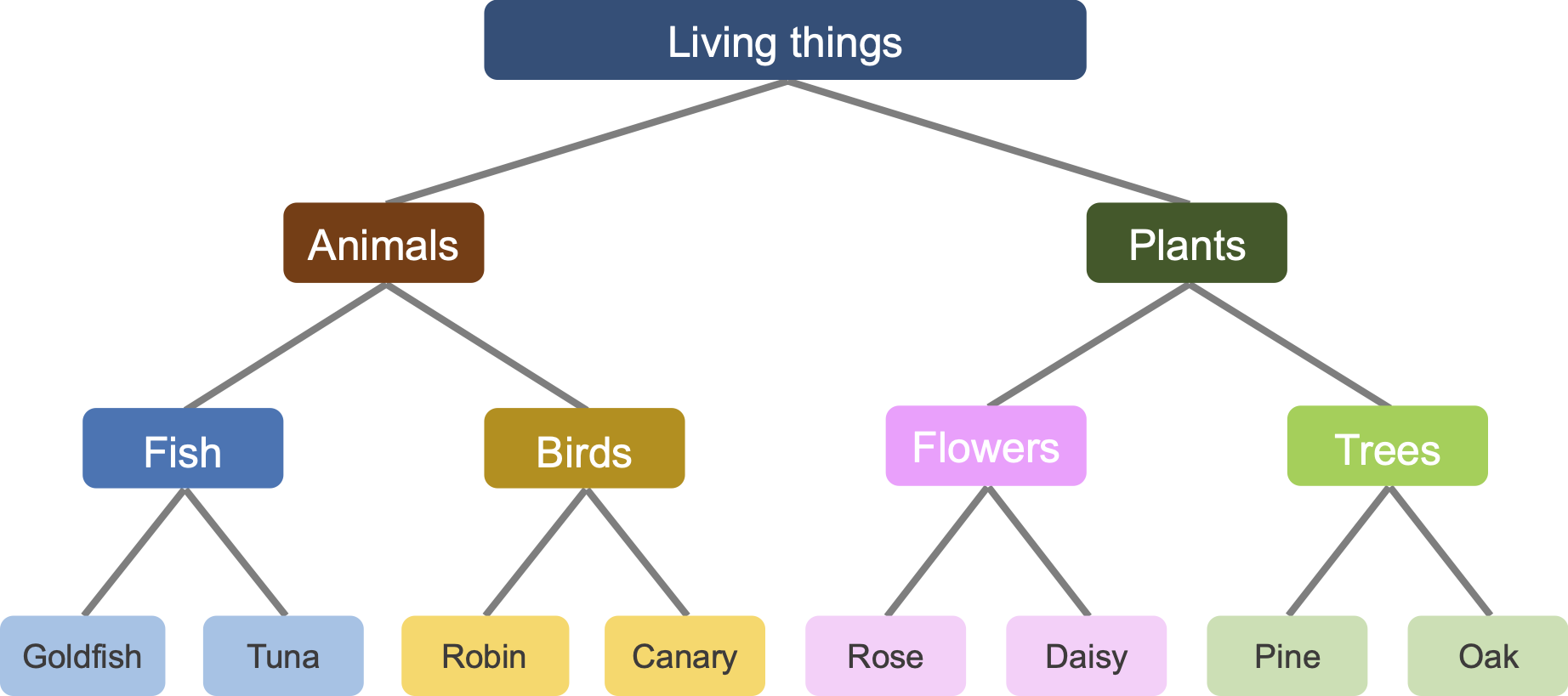
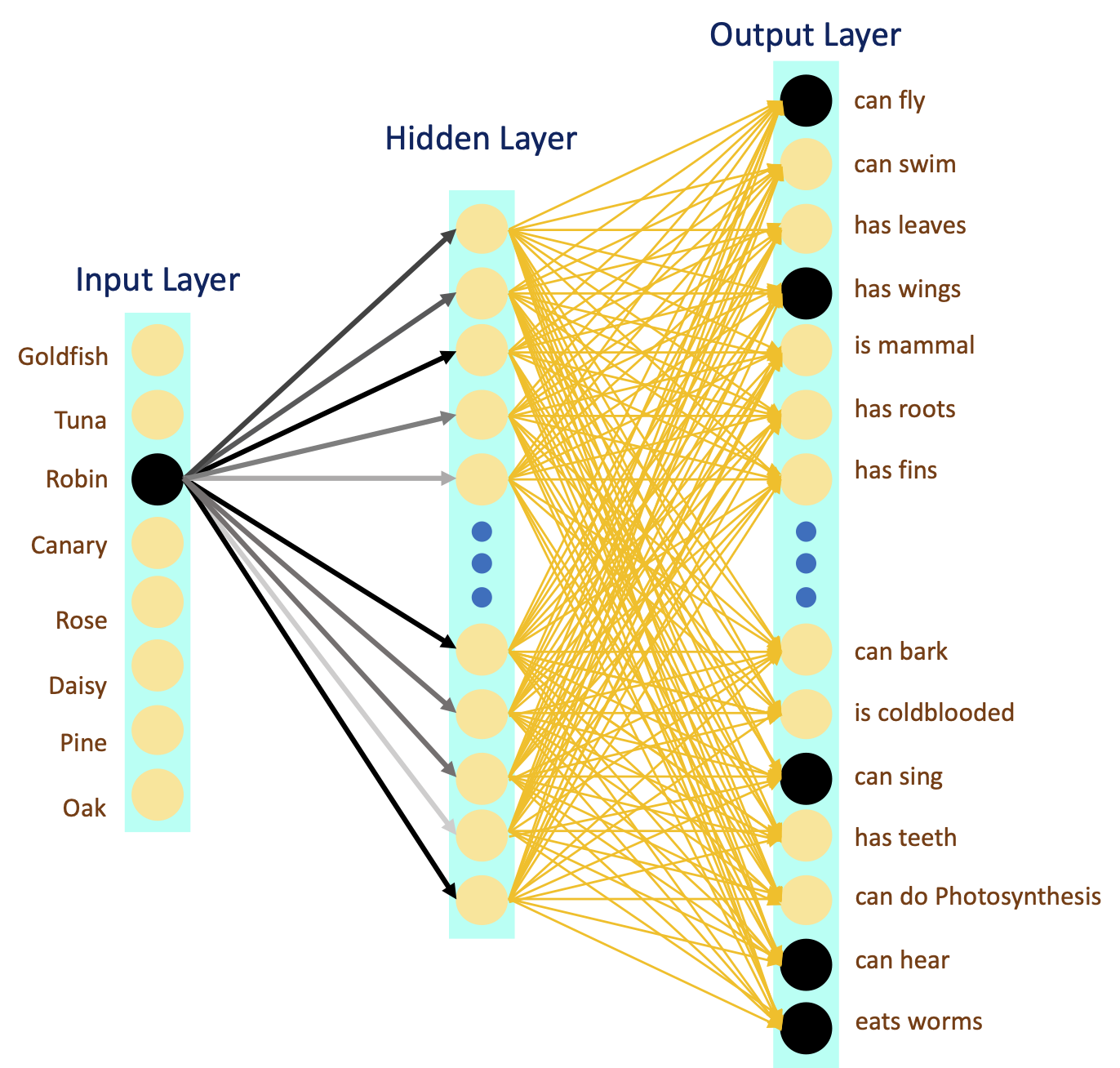
ネットワークへの入力はラベル（つまり名前）であり、出力は特徴（つまり属性）です。例えば、「Goldfish（フナ）」というラベルに対して、ネットワークは「泳げる」「変温動物である」「ひれがある」などの（人工的に作成された）特徴をすべて学習しなければなりません。階層的に構造化されたデータで訓練しているため、ネットワークはGoldfishとTuna（マグロ）がかなり似た特徴を持ち、Robin（コマドリ）はRose（バラ）よりもTunaに共通点が多いというツリー構造も学習できる可能性があります。

# @markdown #### Run to generate and visualize training samples from tree

tree_labels, tree_features = generate_hsd()

# Convert (cast) data from np.ndarray to torch.Tensor
label_tensor = torch.tensor(tree_labels).float()
feature_tensor = torch.tensor(tree_features).float()

item_names = ['Goldfish', 'Tuna', 'Robin', 'Canary',
              'Rose', 'Daisy', 'Pine', 'Oak']
plot_tree_data()

# Dimensions
print("---------------------------------------------------------------")
print("Input Dimension: {}".format(tree_labels.shape[1]))
print("Output Dimension: {}".format(tree_features.shape[1]))
print("Number of samples: {}".format(tree_features.shape[0]))

このチュートリアルを続けるためには、訓練データの前提とタスクが何であるかを理解することが不可欠です。したがって、時間をかけてポッド内でこれらについて議論してください。

このチュートリアルで使用するニューラルネットワーク

インタラクティブデモ1: 深いLNNの訓練

私たちのデータでニューラルネットを訓練するのは簡単です。しかし、次のセルを実行する前に、前回のチュートリアルの訓練損失曲線を思い出してください。

# @markdown #### Make sure you execute this cell to train the network and plot

lr = 100.0  # Learning rate
gamma = 1e-12  # Initialization scale
n_epochs = 250  # Number of epochs
dim_input = 8  # Input dimension = `label_tensor.size(1)`
dim_hidden = 30  # Hidden neurons
dim_output = 10000  # Output dimension = `feature_tensor.size(1)`

# Model instantiation
dlnn_model = LNNet(dim_input, dim_hidden, dim_output)

# Weights re-initialization
initializer_(dlnn_model, gamma)

# Training
losses, *_ = train(dlnn_model,
                  label_tensor,
                  feature_tensor,
                  n_epochs=n_epochs,
                  lr=lr)

# Plotting
plot_loss(losses)

考えてみよう！

なぜこれまで訓練中にこのような「バンプ（山）」を見なかったのでしょうか？そして今後これらを探すべきでしょうか？これらのバンプは何を意味しているのでしょう？

前回のチュートリアルを思い出すと、私たちは常に学習率（ $\eta$ ）と初期化（ $\gamma$ ）に注目しており、それらが最速かつ安定（信頼できる）な収束をもたらすことを目指しています。以下のウィジェットを使って最適な $\eta$ と $\gamma$ を見つけてみてください。特に大きな $\gamma$ を試して、 $\eta$ を調整することでバンプを再現できるか確認してみましょう。

# @markdown #### Make sure you execute this cell to enable the widget!

def loss_lr_init(lr, gamma):
  """
  Trains and plots the loss evolution

  Args:
    lr: float
      Learning rate
    gamma: float
      Initialization scale

  Returns:
    Nothing
  """
  n_epochs = 250  # Number of epochs
  dim_input = 8  # Input dimension = `label_tensor.size(1)`
  dim_hidden = 30  # Hidden neurons
  dim_output = 10000  # Output dimension = `feature_tensor.size(1)`

  # Model instantiation
  dlnn_model = LNNet(dim_input, dim_hidden, dim_output)

  # Weights re-initialization
  initializer_(dlnn_model, gamma)

  losses, *_ = train(dlnn_model,
                    label_tensor,
                    feature_tensor,
                    n_epochs=n_epochs,
                    lr=lr)

  plot_loss(losses)

_ = interact(loss_lr_init,
             lr = FloatSlider(min=1.0, max=200.0,
                              step=1.0, value=100.0,
                              continuous_update=False,
                              readout_format='.1f',
                              description='eta'),
             epochs = fixed(250),
             gamma = FloatLogSlider(min=-15, max=1,
                                    step=1, value=1e-12, base=10,
                                    continuous_update=False,
                                    description='gamma')
             )

# @title Submit your feedback
content_review(f"{feedback_prefix}_Training_the_deep_LNN_Interactive_Demo")

セクション2: 特異値分解（SVD）

所要時間の目安: 約20分

# @title Video 2: SVD
from ipywidgets import widgets
from IPython.display import YouTubeVideo
from IPython.display import IFrame
from IPython.display import display


class PlayVideo(IFrame):
  def __init__(self, id, source, page=1, width=400, height=300, **kwargs):
    self.id = id
    if source == 'Bilibili':
      src = f'https://player.bilibili.com/player.html?bvid={id}&page={page}'
    elif source == 'Osf':
      src = f'https://mfr.ca-1.osf.io/render?url=https://osf.io/download/{id}/?direct%26mode=render'
    super(PlayVideo, self).__init__(src, width, height, **kwargs)


def display_videos(video_ids, W=400, H=300, fs=1):
  tab_contents = []
  for i, video_id in enumerate(video_ids):
    out = widgets.Output()
    with out:
      if video_ids[i][0] == 'Youtube':
        video = YouTubeVideo(id=video_ids[i][1], width=W,
                             height=H, fs=fs, rel=0)
        print(f'Video available at https://youtube.com/watch?v={video.id}')
      else:
        video = PlayVideo(id=video_ids[i][1], source=video_ids[i][0], width=W,
                          height=H, fs=fs, autoplay=False)
        if video_ids[i][0] == 'Bilibili':
          print(f'Video available at https://www.bilibili.com/video/{video.id}')
        elif video_ids[i][0] == 'Osf':
          print(f'Video available at https://osf.io/{video.id}')
      display(video)
    tab_contents.append(out)
  return tab_contents


video_ids = [('Youtube', '18oNWRziskM'), ('Bilibili', 'BV1bw411R7DJ')]
tab_contents = display_videos(video_ids, W=854, H=480)
tabs = widgets.Tab()
tabs.children = tab_contents
for i in range(len(tab_contents)):
  tabs.set_title(i, video_ids[i][0])
display(tabs)

# @title Submit your feedback
content_review(f"{feedback_prefix}_SVD_Video")

このセクションでは、先ほど見た学習（訓練）ダイナミクスを研究します。まず、線形ニューラルネットワークは連続した行列の掛け算を行っていることを知っておくべきです。これは次のように簡略化できます。

\begin{align}
$\mathbf{y}$ &= $\mathbf{W}_{L}$ ~ $\mathbf{W}_{L-1}$ ~ $\dots$ ~ $\mathbf{W}_{1}$ ~ $\mathbf{x}$ \
&= $\left(\prod_{i=1}^{L}{\mathbf{W}_{i}}\right)$ ~ $\mathbf{x}$ \
&= $\mathbf{W}_{tot}$ ~ $\mathbf{x} \end{align}$

ここで $L$ はネットワークの層数を表します。

Saxe et al. (2013)は、深いLNNの非線形学習ダイナミクスを解析・理解するために、特異値分解（SVD）を用いて $\mathbf{W}_{tot}$ を直交ベクトルに分解できることを示しました。ベクトルの直交性はそれらの「個別性（独立性）」を保証します。つまり、深くて幅広いLNNを複数の深くて狭いLNNに分解でき、それぞれの活動が互いに絡み合わないようにできるのです。

SVDの簡単な紹介

任意の実数値行列 $A$ （そう、どんな行列でも）は3つの行列に分解（因数分解）できます：

\mathbf{A} = \mathbf{U} \mathbf{Σ} \mathbf{V}^{\top}

ここで $U$ は直交行列、 $\Sigma$ は対角行列、 $V$ も直交行列です。 $\Sigma$ の対角要素は特異値と呼ばれます。

SVDと固有値分解（EVD）の主な違いは、EVDは $A$ が正方行列である必要があり、固有ベクトルが直交するとは限らない点です。

もっと学びたい方には、素晴らしいGilbert Strangによる特異値分解（SVD）の動画を強くお勧めします。

コーディング演習2: SVD（任意）

目的は、各エポックで $\mathbf{W}_{tot}$ に対してSVDを実行し、訓練中の特異値（モード）を記録することです。

関数ex_net_svdを完成させてください。まず $\mathbf{W}_{tot} = \prod_{i=1}^{L}{\mathbf{W}_{i}}$ を計算し、最後に $\mathbf{W}_{tot}$ に対してSVDを実行します。NumPyのnp.linalg.svdではなく、PyTorchのtorch.svdを使用してください。

def ex_net_svd(model, in_dim):
  """
  Performs a Singular Value Decomposition on a given model weights

  Args:
    model: torch.nn.Module
      Neural network model
    in_dim: int
      The input dimension of the model

  Returns:
    U: torch.tensor
      Orthogonal matrix
    Σ: torch.tensor
      Diagonal matrix
    V: torch.tensor
      Orthogonal matrix
  """
  W_tot = torch.eye(in_dim)
  for weight in model.parameters():
    #################################################
    ## Calculate the W_tot by multiplication of all weights
    # and then perform SVD on the W_tot using pytorch's `torch.svd`
    # Complete the function and remove or comment the line below
    raise NotImplementedError("Function `ex_net_svd`")
    #################################################
    W_tot = ...
  U, Σ, V = ...
  return U, Σ, V


## Uncomment and run
# test_net_svd_ex(SEED)

解答を見る$

# @title Submit your feedback
content_review(f"{feedback_prefix}_SVD_Exercise")

# @markdown #### Make sure you execute this cell to train the network and plot

lr = 100.0  # Learning rate
gamma = 1e-12  # Initialization scale
n_epochs = 250  # Number of epochs
dim_input = 8  # Input dimension = `label_tensor.size(1)`
dim_hidden = 30  # Hidden neurons
dim_output = 10000  # Output dimension = `feature_tensor.size(1)`

# Model instantiation
dlnn_model = LNNet(dim_input, dim_hidden, dim_output)

# Weights re-initialization
initializer_(dlnn_model, gamma)

# Training
losses, modes, *_ = train(dlnn_model,
                          label_tensor,
                          feature_tensor,
                          n_epochs=n_epochs,
                          lr=lr)

plot_loss_sv_twin(losses, modes)

考えてみよう！

固有値分解では、固有ベクトルによって説明される分散の量は対応する固有値に比例します。ではSVDではどうでしょう？勾配降下法は、より多くの情報を持つ（より高い特異値を持つ）特徴を最初に学習するようにネットワークを導いていることがわかります！

# @title Submit your feedback
content_review(f"{feedback_prefix}_SVD_Discussion")

# @title Video 3: SVD - Discussion
from ipywidgets import widgets
from IPython.display import YouTubeVideo
from IPython.display import IFrame
from IPython.display import display


class PlayVideo(IFrame):
  def __init__(self, id, source, page=1, width=400, height=300, **kwargs):
    self.id = id
    if source == 'Bilibili':
      src = f'https://player.bilibili.com/player.html?bvid={id}&page={page}'
    elif source == 'Osf':
      src = f'https://mfr.ca-1.osf.io/render?url=https://osf.io/download/{id}/?direct%26mode=render'
    super(PlayVideo, self).__init__(src, width, height, **kwargs)


def display_videos(video_ids, W=400, H=300, fs=1):
  tab_contents = []
  for i, video_id in enumerate(video_ids):
    out = widgets.Output()
    with out:
      if video_ids[i][0] == 'Youtube':
        video = YouTubeVideo(id=video_ids[i][1], width=W,
                             height=H, fs=fs, rel=0)
        print(f'Video available at https://youtube.com/watch?v={video.id}')
      else:
        video = PlayVideo(id=video_ids[i][1], source=video_ids[i][0], width=W,
                          height=H, fs=fs, autoplay=False)
        if video_ids[i][0] == 'Bilibili':
          print(f'Video available at https://www.bilibili.com/video/{video.id}')
        elif video_ids[i][0] == 'Osf':
          print(f'Video available at https://osf.io/{video.id}')
      display(video)
    tab_contents.append(out)
  return tab_contents


video_ids = [('Youtube', 'JEbRPPG2kUI'), ('Bilibili', 'BV1t54y1J7Tb')]
tab_contents = display_videos(video_ids, W=854, H=480)
tabs = widgets.Tab()
tabs.children = tab_contents
for i in range(len(tab_contents)):
  tabs.set_title(i, video_ids[i][0])
display(tabs)

# @title Submit your feedback
content_review(f"{feedback_prefix}_SVD_Discussion_Video")

セクション3: 表現類似性解析（RSA）

所要時間の目安: 約20分

# @title Video 4: RSA
from ipywidgets import widgets
from IPython.display import YouTubeVideo
from IPython.display import IFrame
from IPython.display import display


class PlayVideo(IFrame):
  def __init__(self, id, source, page=1, width=400, height=300, **kwargs):
    self.id = id
    if source == 'Bilibili':
      src = f'https://player.bilibili.com/player.html?bvid={id}&page={page}'
    elif source == 'Osf':
      src = f'https://mfr.ca-1.osf.io/render?url=https://osf.io/download/{id}/?direct%26mode=render'
    super(PlayVideo, self).__init__(src, width, height, **kwargs)


def display_videos(video_ids, W=400, H=300, fs=1):
  tab_contents = []
  for i, video_id in enumerate(video_ids):
    out = widgets.Output()
    with out:
      if video_ids[i][0] == 'Youtube':
        video = YouTubeVideo(id=video_ids[i][1], width=W,
                             height=H, fs=fs, rel=0)
        print(f'Video available at https://youtube.com/watch?v={video.id}')
      else:
        video = PlayVideo(id=video_ids[i][1], source=video_ids[i][0], width=W,
                          height=H, fs=fs, autoplay=False)
        if video_ids[i][0] == 'Bilibili':
          print(f'Video available at https://www.bilibili.com/video/{video.id}')
        elif video_ids[i][0] == 'Osf':
          print(f'Video available at https://osf.io/{video.id}')
      display(video)
    tab_contents.append(out)
  return tab_contents


video_ids = [('Youtube', 'YOs1yffysX8'), ('Bilibili', 'BV19f4y157zD')]
tab_contents = display_videos(video_ids, W=854, H=480)
tabs = widgets.Tab()
tabs.children = tab_contents
for i in range(len(tab_contents)):
  tabs.set_title(i, video_ids[i][0])
display(tabs)

# @title Submit your feedback
content_review(f"{feedback_prefix}_RSA_Video")

前のセクションは興味深い指摘で終わりました。SVDは、深い「幅広い」線形ニューラルネットを8つの深い「狭い」線形ニューラルネットに分解するのに役立ちました。

最初の狭いネット（最大特異値）は最も速く収束し、最後の4つの狭いネットはほぼ同時に収束し、最も小さい特異値を持っています。特異値の大きい狭いネットは「生物」と「物体」の違いを学習し、特異値の小さい別の狭いネットは魚と鳥の違いを学習しているのかもしれません。この仮説をどうやって検証できるでしょうか？

表現類似性解析（Representational Similarity Analysis, RSA）は、ネットワークの内部表現を理解するのに役立つアプローチです。主な考え方は、ネットワークに類似した入力が与えられたとき、隠れユニット（ニューロン）の活動が類似していなければならないということです。階層的に構造化されたデータセットの場合、隠れ層のニューロンの活動はツナとカナリアでより類似し、ツナとオークではあまり類似しないことが期待されます。

類似度の測定には、古典的なドット積（スカラー積）、すなわちコサイン類似度を使うことができます。複数のベクトル間のドット積を計算する場合（今回のケース）、単純に行列積を使えばよいです。したがって、複数入力（バッチ）に対する表現類似性行列は以下のように計算できます：

RSM = \mathbf{H} \mathbf{H}^{\top}

ここで、 $\mathbf{H} = \mathbf{X} \mathbf{W_1}$ は与えられたバッチ $\mathbf{X}$ に対する隠れニューロンの活動です。

コーディング演習3: RSA（任意）

課題はシンプルです。各入力 $\mathbf{x}$ に対して隠れ層の活動 $~\mathbf{h} = \mathbf{x} ~\mathbf{W_1}$ の類似度を測定します。

もし毎回のイテレーションでRSAを実行すれば、表現学習の進化も観察できます。

def ex_net_rsm(h):
  """
  Calculates the Representational Similarity Matrix

  Arg:
    h: torch.Tensor
      Activity of a hidden layer

  Returns:
    rsm: torch.Tensor
      Representational Similarity Matrix
  """
  #################################################
  ## Calculate the Representational Similarity Matrix
  # Complete the function and remove or comment the line below
  raise NotImplementedError("Function `ex_net_rsm`")
  #################################################
  rsm = ...
  return rsm


## Uncomment and run
# test_net_rsm_ex(SEED)

解答はこちら$

これで、損失、モード、RSMを毎イテレーション記録しながらモデルを訓練できます。まずはエポックスライダーを使って、デフォルトの学習率 ( $\eta$ ) と初期化 ( $\gamma$ ) を変えずにRSMの進化を探索してください。その後、前回と同様に $\eta$ と $\gamma$ を大きく設定し、表現の逐次的な構造学習が再現できるか試してみましょう。

#@markdown #### Make sure you execute this cell to enable widgets

def loss_svd_rsm_lr_gamma(lr, gamma, i_ep):
  """
  Widget to record loss/mode/RSM at every iteration

  Args:
    lr: float
      Learning rate
    gamma: float
      Initialization scale
    i_ep: int
      Which epoch to show

  Returns:
    Nothing
  """
  n_epochs = 250  # Number of epochs
  dim_input = 8  # Input dimension = `label_tensor.size(1)`
  dim_hidden = 30  # Hidden neurons
  dim_output = 10000  # Output dimension = `feature_tensor.size(1)`

  # Model instantiation
  dlnn_model = LNNet(dim_input, dim_hidden, dim_output)

  # Weights re-initialization
  initializer_(dlnn_model, gamma)

  # Training
  losses, modes, rsms, _ = train(dlnn_model,
                                 label_tensor,
                                 feature_tensor,
                                 n_epochs=n_epochs,
                                 lr=lr)
  plot_loss_sv_rsm(losses, modes, rsms, i_ep)

i_ep_slider = IntSlider(min=10, max=241, step=1, value=61,
                        continuous_update=False,
                        description='Epoch',
                        layout=Layout(width='630px'))

lr_slider = FloatSlider(min=20.0, max=200.0, step=1.0, value=100.0,
                        continuous_update=False,
                        readout_format='.1f',
                        description='eta')

gamma_slider = FloatLogSlider(min=-15, max=1, step=1,
                              value=1e-12, base=10,
                              continuous_update=False,
                              description='gamma')

widgets_ui = VBox([lr_slider, gamma_slider, i_ep_slider])

widgets_out = interactive_output(loss_svd_rsm_lr_gamma,
                                 {'lr': lr_slider,
                                  'gamma': gamma_slider,
                                  'i_ep': i_ep_slider})

display(widgets_ui, widgets_out)

もう少し分析してみましょう。深いニューラルネットは単なる単純なマッピング（ルックアップテーブル）ではなく、表現を学習しています。これが深層ニューラルネットの優れた一般化能力や転移学習能力の理由と考えられています。予想通り、隠れ層のないニューラルネットは、極めて小さい初期化でも表現学習ができません。

# @title Submit your feedback
content_review(f"{feedback_prefix}_RSA_Exercise")

# @title Video 5: RSA - Discussion
from ipywidgets import widgets
from IPython.display import YouTubeVideo
from IPython.display import IFrame
from IPython.display import display


class PlayVideo(IFrame):
  def __init__(self, id, source, page=1, width=400, height=300, **kwargs):
    self.id = id
    if source == 'Bilibili':
      src = f'https://player.bilibili.com/player.html?bvid={id}&page={page}'
    elif source == 'Osf':
      src = f'https://mfr.ca-1.osf.io/render?url=https://osf.io/download/{id}/?direct%26mode=render'
    super(PlayVideo, self).__init__(src, width, height, **kwargs)


def display_videos(video_ids, W=400, H=300, fs=1):
  tab_contents = []
  for i, video_id in enumerate(video_ids):
    out = widgets.Output()
    with out:
      if video_ids[i][0] == 'Youtube':
        video = YouTubeVideo(id=video_ids[i][1], width=W,
                             height=H, fs=fs, rel=0)
        print(f'Video available at https://youtube.com/watch?v={video.id}')
      else:
        video = PlayVideo(id=video_ids[i][1], source=video_ids[i][0], width=W,
                          height=H, fs=fs, autoplay=False)
        if video_ids[i][0] == 'Bilibili':
          print(f'Video available at https://www.bilibili.com/video/{video.id}')
        elif video_ids[i][0] == 'Osf':
          print(f'Video available at https://osf.io/{video.id}')
      display(video)
    tab_contents.append(out)
  return tab_contents


video_ids = [('Youtube', 'vprldATyq1o'), ('Bilibili', 'BV18y4y1j7Xr')]
tab_contents = display_videos(video_ids, W=854, H=480)
tabs = widgets.Tab()
tabs.children = tab_contents
for i in range(len(tab_contents)):
  tabs.set_title(i, video_ids[i][0])
display(tabs)

# @title Submit your feedback
content_review(f"{feedback_prefix}_RSA_Discussion_Video")

セクション4: 幻想的相関

所要時間の目安: 約20～30分

# @title Video 6: Illusory Correlations
from ipywidgets import widgets
from IPython.display import YouTubeVideo
from IPython.display import IFrame
from IPython.display import display


class PlayVideo(IFrame):
  def __init__(self, id, source, page=1, width=400, height=300, **kwargs):
    self.id = id
    if source == 'Bilibili':
      src = f'https://player.bilibili.com/player.html?bvid={id}&page={page}'
    elif source == 'Osf':
      src = f'https://mfr.ca-1.osf.io/render?url=https://osf.io/download/{id}/?direct%26mode=render'
    super(PlayVideo, self).__init__(src, width, height, **kwargs)


def display_videos(video_ids, W=400, H=300, fs=1):
  tab_contents = []
  for i, video_id in enumerate(video_ids):
    out = widgets.Output()
    with out:
      if video_ids[i][0] == 'Youtube':
        video = YouTubeVideo(id=video_ids[i][1], width=W,
                             height=H, fs=fs, rel=0)
        print(f'Video available at https://youtube.com/watch?v={video.id}')
      else:
        video = PlayVideo(id=video_ids[i][1], source=video_ids[i][0], width=W,
                          height=H, fs=fs, autoplay=False)
        if video_ids[i][0] == 'Bilibili':
          print(f'Video available at https://www.bilibili.com/video/{video.id}')
        elif video_ids[i][0] == 'Osf':
          print(f'Video available at https://osf.io/{video.id}')
      display(video)
    tab_contents.append(out)
  return tab_contents


video_ids = [('Youtube', 'RxsAvyIoqEo'), ('Bilibili', 'BV1vv411E7Sq')]
tab_contents = display_videos(video_ids, W=854, H=480)
tabs = widgets.Tab()
tabs.children = tab_contents
for i in range(len(tab_contents)):
  tabs.set_title(i, video_ids[i][0])
display(tabs)

# @title Submit your feedback
content_review(f"{feedback_prefix}_IllusoryCorrelations_Video")

訓練損失曲線を思い出しましょう。しばしば長い停滞（重みが鞍点にとどまる）があり、その後に急激な減少が起こりました。非常に深く複雑なニューラルネットでは、このような停滞が数時間続くこともあり、私たちは「これ以上は良くならない」と思って訓練を止めたくなります。訓練の「未熟な中断」の副作用の一つは、ネットワークが幻想的相関を見つけ（学習し）てしまうことです。

これをよりよく理解するために、次のデモンストレーションと演習を行いましょう。

デモンストレーション: 幻想的相関

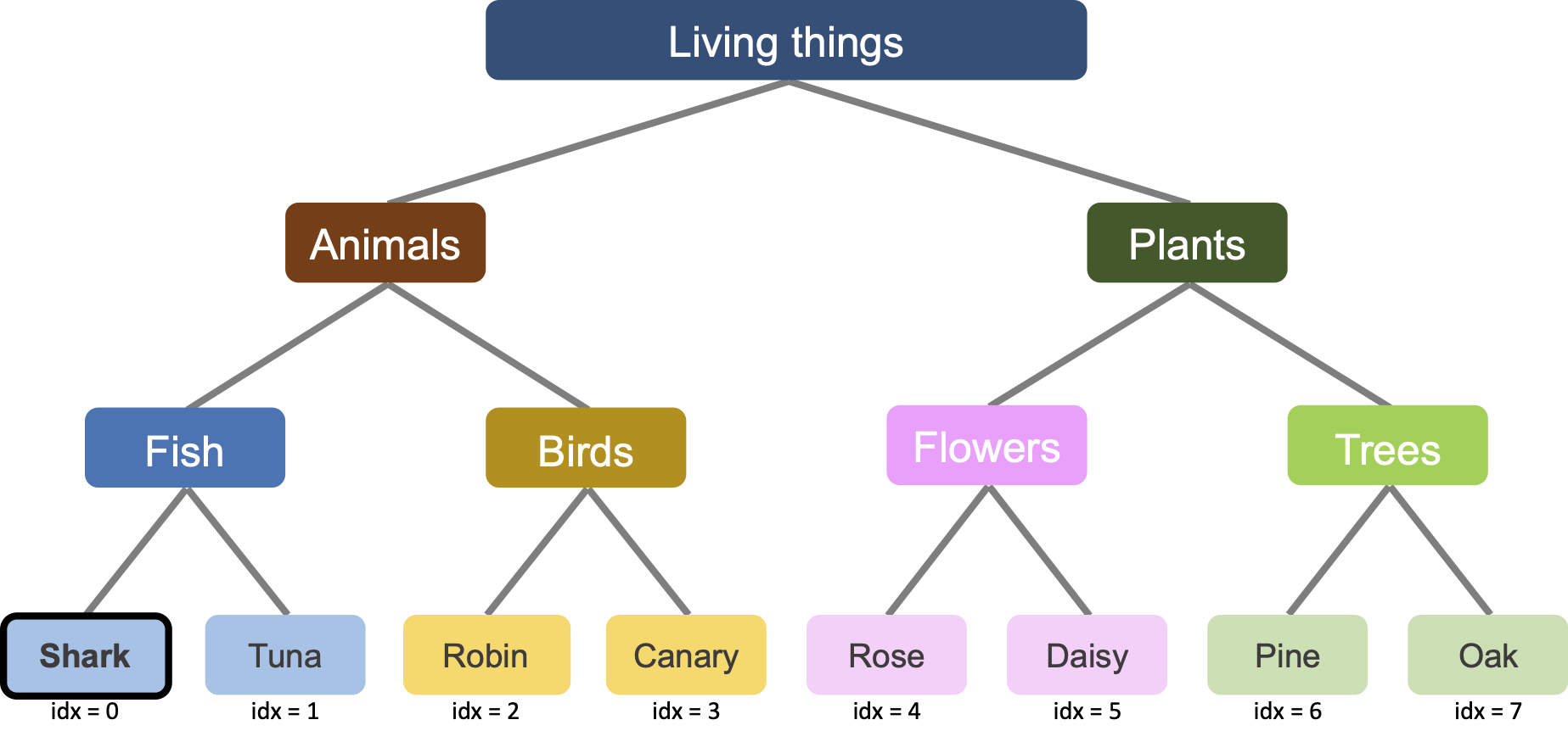
元のデータセットには4種類の動物がいます：カナリア、コマドリ、金魚、ツナ。これらの動物はすべて骨を持っています。したがって、「骨がある」という特徴を含めると、ネットワークは動物と植物の区別を学習する第2段階（第2の山、第2のモード収束）でこれを学習します。

もし金魚の代わりにサメがデータセットに入っていたらどうでしょうか。サメは骨を持っていません（骨格は軟骨でできており、本物の骨より軽く柔軟です）。すると、「骨がある」特徴はツナ、コマドリ、カナリアでは真（+1）ですが、植物とサメでは偽（-1）になります。ネットワークはどうなるでしょうか。

まず、新しい特徴をターゲットに追加します。次にLNNを訓練し、各エポックで「サメが骨を持つか」のネットワーク予測を記録します。

# Sampling new data from the tree
tree_labels, tree_features = generate_hsd()

# Replacing Goldfish with Shark
item_names = ['Shark', 'Tuna', 'Robin', 'Canary',
              'Rose', 'Daisy', 'Pine', 'Oak']

# Index of label to record
illusion_idx = 0  # Shark is the first element

# The new feature (has bones) vector
new_feature = [-1, 1, 1, 1, -1, -1, -1, -1]
its_label = 'has_bones'

# Adding feature has_bones to the feature array
tree_features = add_feature(tree_features, new_feature)

# Plotting
plot_tree_data(item_names, tree_features, its_label)

上のプロットの最後の列に新しい特徴が示されています。

新しいデータでネットワークを訓練し、訓練中にサメ（インデックス0）ラベルの「骨がある」特徴（最後の特徴、インデックス-1）に対するネットワークの予測（出力）を記録しましょう。

以下は、訓練ループ内で illusory_i 番目のラベルと最後の (-1) 特徴に対するネットワーク予測を追跡するコードの一部です：

pred_ij = predictions.detach()[illusory_i, -1]

#@markdown #### Make sure you execute this cell to train the network and plot

# Convert (cast) data from np.ndarray to torch.Tensor
label_tensor = torch.tensor(tree_labels).float()
feature_tensor = torch.tensor(tree_features).float()

lr = 100.0  # Learning rate
gamma = 1e-12  # Initialization scale
n_epochs = 250  # Number of epochs
dim_input = 8  # Input dimension = `label_tensor.size(1)`
dim_hidden = 30  # Hidden neurons
dim_output = feature_tensor.size(1)

# Model instantiation
dlnn_model = LNNet(dim_input, dim_hidden, dim_output)

# Weights re-initialization
initializer_(dlnn_model, gamma)

# Training
_, modes, _, ill_predictions = train(dlnn_model,
                                     label_tensor,
                                     feature_tensor,
                                     n_epochs=n_epochs,
                                     lr=lr,
                                     illusory_i=illusion_idx)

# Label for the plot
ill_label = f"Prediction for {item_names[illusion_idx]} {its_label}"

# Plotting
plot_ills_sv_twin(ill_predictions, modes, ill_label)

ネットワークは最初、サメが骨を持つという「幻想的相関」を学習し始め、後のエポックでより深い表現を学習するにつれて、その幻想的相関を超えて理解できるようになるようです。重要なのは、私たちはネットワークにサメが骨を持つというデータを一度も提示していないということです。

演習4: 幻想的相関

この演習は、幻想的相関のアイデアを探求するためのものです。医療、自然、あるいは社会的な幻想的相関の例を考え、深い線形ニューラルネットの学習能力を試してみてください。

重要な注意：生成されるデータはツリーのラベルとは独立しているため、名前は便宜上のものです。

以下は「非人間の生物は話さない」という例です。 {edit} と記された行はあなたが例を変更するための箇所です。

# Sampling new data from the tree
tree_labels, tree_features = generate_hsd()

# {edit} Replacing Canary with Parrot
item_names = ['Goldfish', 'Tuna', 'Robin', 'Parrot',
              'Rose', 'Daisy', 'Pine', 'Oak']

# {edit} Index of label to record
illusion_idx = 3  # Parrot is the fourth element

# {edit} The new feature (cannot speak) vector
new_feature = [1, 1, 1, -1, 1, 1, 1, 1]
its_label = 'cannot_speak'

# Adding feature has_bones to the feature array
tree_features = add_feature(tree_features, new_feature)

# Plotting
plot_tree_data(item_names, tree_features, its_label)

# @markdown #### Make sure you execute this cell to train the network and plot

# Convert (cast) data from np.ndarray to torch.Tensor
label_tensor = torch.tensor(tree_labels).float()
feature_tensor = torch.tensor(tree_features).float()

lr = 100.0  # Learning rate
gamma = 1e-12  # Initialization scale
n_epochs = 250  # Number of epochs
dim_input = 8  # Input dimension = `label_tensor.size(1)`
dim_hidden = 30  # Hidden neurons
dim_output = feature_tensor.size(1)

# Model instantiation
dlnn_model = LNNet(dim_input, dim_hidden, dim_output)

# Weights re-initialization
initializer_(dlnn_model, gamma)

# Training
_, modes, _, ill_predictions = train(dlnn_model,
                                     label_tensor,
                                     feature_tensor,
                                     n_epochs=n_epochs,
                                     lr=lr,
                                     illusory_i=illusion_idx)

# Label for the plot
ill_label = f"Prediction for {item_names[illusion_idx]} {its_label}"

# Plotting
plot_ills_sv_twin(ill_predictions, modes, ill_label)

# @title Submit your feedback
content_review(f"{feedback_prefix}_Illusory_Correlations_Exercise")

# @title Video 7: Illusory Correlations - Discussion
from ipywidgets import widgets
from IPython.display import YouTubeVideo
from IPython.display import IFrame
from IPython.display import display


class PlayVideo(IFrame):
  def __init__(self, id, source, page=1, width=400, height=300, **kwargs):
    self.id = id
    if source == 'Bilibili':
      src = f'https://player.bilibili.com/player.html?bvid={id}&page={page}'
    elif source == 'Osf':
      src = f'https://mfr.ca-1.osf.io/render?url=https://osf.io/download/{id}/?direct%26mode=render'
    super(PlayVideo, self).__init__(src, width, height, **kwargs)


def display_videos(video_ids, W=400, H=300, fs=1):
  tab_contents = []
  for i, video_id in enumerate(video_ids):
    out = widgets.Output()
    with out:
      if video_ids[i][0] == 'Youtube':
        video = YouTubeVideo(id=video_ids[i][1], width=W,
                             height=H, fs=fs, rel=0)
        print(f'Video available at https://youtube.com/watch?v={video.id}')
      else:
        video = PlayVideo(id=video_ids[i][1], source=video_ids[i][0], width=W,
                          height=H, fs=fs, autoplay=False)
        if video_ids[i][0] == 'Bilibili':
          print(f'Video available at https://www.bilibili.com/video/{video.id}')
        elif video_ids[i][0] == 'Osf':
          print(f'Video available at https://osf.io/{video.id}')
      display(video)
    tab_contents.append(out)
  return tab_contents


video_ids = [('Youtube', '6VLHKQjQJmI'), ('Bilibili', 'BV1vv411E7rg')]
tab_contents = display_videos(video_ids, W=854, H=480)
tabs = widgets.Tab()
tabs.children = tab_contents
for i in range(len(tab_contents)):
  tabs.set_title(i, video_ids[i][0])
display(tabs)

# @title Submit your feedback
content_review(f"{feedback_prefix}_Illusory_Correlations_Discussion_Video")

サマリー

コースの2日目が終了しました。したがって、線形ディープラーニングの日の第3回チュートリアルでは、より高度なトピックを学びました。最初に深い線形ニューラルネットワークを実装し、その後、特異値分解という線形代数のツールを使ってその学習ダイナミクスを調べました。次に、表現類似性解析と錯覚的相関について学びました。

# @title Video 8: Outro
from ipywidgets import widgets
from IPython.display import YouTubeVideo
from IPython.display import IFrame
from IPython.display import display


class PlayVideo(IFrame):
  def __init__(self, id, source, page=1, width=400, height=300, **kwargs):
    self.id = id
    if source == 'Bilibili':
      src = f'https://player.bilibili.com/player.html?bvid={id}&page={page}'
    elif source == 'Osf':
      src = f'https://mfr.ca-1.osf.io/render?url=https://osf.io/download/{id}/?direct%26mode=render'
    super(PlayVideo, self).__init__(src, width, height, **kwargs)


def display_videos(video_ids, W=400, H=300, fs=1):
  tab_contents = []
  for i, video_id in enumerate(video_ids):
    out = widgets.Output()
    with out:
      if video_ids[i][0] == 'Youtube':
        video = YouTubeVideo(id=video_ids[i][1], width=W,
                             height=H, fs=fs, rel=0)
        print(f'Video available at https://youtube.com/watch?v={video.id}')
      else:
        video = PlayVideo(id=video_ids[i][1], source=video_ids[i][0], width=W,
                          height=H, fs=fs, autoplay=False)
        if video_ids[i][0] == 'Bilibili':
          print(f'Video available at https://www.bilibili.com/video/{video.id}')
        elif video_ids[i][0] == 'Osf':
          print(f'Video available at https://osf.io/{video.id}')
      display(video)
    tab_contents.append(out)
  return tab_contents


video_ids = [('Youtube', 'N2szOIsKyXE'), ('Bilibili', 'BV1AL411n7ns')]
tab_contents = display_videos(video_ids, W=854, H=480)
tabs = widgets.Tab()
tabs.children = tab_contents
for i in range(len(tab_contents)):
  tabs.set_title(i, video_ids[i][0])
display(tabs)

# @title Submit your feedback
content_review(f"{feedback_prefix}_Outro_Video")

ボーナス

所要時間の目安: 約20～30分

# @title Video 9: Linear Regression
from ipywidgets import widgets
from IPython.display import YouTubeVideo
from IPython.display import IFrame
from IPython.display import display


class PlayVideo(IFrame):
  def __init__(self, id, source, page=1, width=400, height=300, **kwargs):
    self.id = id
    if source == 'Bilibili':
      src = f'https://player.bilibili.com/player.html?bvid={id}&page={page}'
    elif source == 'Osf':
      src = f'https://mfr.ca-1.osf.io/render?url=https://osf.io/download/{id}/?direct%26mode=render'
    super(PlayVideo, self).__init__(src, width, height, **kwargs)


def display_videos(video_ids, W=400, H=300, fs=1):
  tab_contents = []
  for i, video_id in enumerate(video_ids):
    out = widgets.Output()
    with out:
      if video_ids[i][0] == 'Youtube':
        video = YouTubeVideo(id=video_ids[i][1], width=W,
                             height=H, fs=fs, rel=0)
        print(f'Video available at https://youtube.com/watch?v={video.id}')
      else:
        video = PlayVideo(id=video_ids[i][1], source=video_ids[i][0], width=W,
                          height=H, fs=fs, autoplay=False)
        if video_ids[i][0] == 'Bilibili':
          print(f'Video available at https://www.bilibili.com/video/{video.id}')
        elif video_ids[i][0] == 'Osf':
          print(f'Video available at https://osf.io/{video.id}')
      display(video)
    tab_contents.append(out)
  return tab_contents


video_ids = [('Youtube', 'uULOAbhYaaE'), ('Bilibili', 'BV1Pf4y1L71L')]
tab_contents = display_videos(video_ids, W=854, H=480)
tabs = widgets.Tab()
tabs.children = tab_contents
for i in range(len(tab_contents)):
  tabs.set_title(i, video_ids[i][0])
display(tabs)

# @title Submit your feedback
content_review(f"{feedback_prefix}_Linear_Regression_Bonus_Video")

セクション 5.1: 線形回帰

一般に、回帰とは、1つ（または複数）の独立変数（特徴量）と1つ（または複数）の従属変数（ラベル）との間の写像（関係）をモデル化する一連の手法を指します。例えば、カレンダーの日付、GPS座標、時刻（独立変数）が気温（従属変数）に与える相対的な影響を調べたい場合です。一方で、回帰は予測分析にも用いられます。したがって、独立変数は予測子とも呼ばれます。モデルに複数の予測子が含まれる場合は重回帰、複数の従属変数が含まれる場合は多変量回帰と呼ばれます。回帰問題は、数値（通常は連続値）を予測したい場合に頻繁に現れます。

独立変数はベクトル $\mathbf{x} \in \mathbb{R}^M$ にまとめられ、ここで $M$ は独立変数の数を示します。一方、従属変数はベクトル $\mathbf{y} \in \mathbb{R}^N$ にまとめられ、 $N$ は従属変数の数を示します。そして、それらの間の写像は重み行列 $\mathbf{W} \in \mathbb{R}^{N \times M}$ とバイアスベクトル $\mathbf{b} \in \mathbb{R}^N$ によって表されます（アフィン写像への一般化）。

多変量回帰モデルは次のように書けます:

\mathbf{y} = \mathbf{W} ~ \mathbf{x} + \mathbf{b}

また、行列形式では次のように表せます:

\begin{bmatrix} y_{1} \\ y_{2} \\ \vdots \\ y_{N} \\ \end{bmatrix} = \begin{bmatrix} w_{1,1} & w_{1,2} & \dots & w_{1,M} \\ w_{2,1} & w_{2,2} & \dots & w_{2,M} \\ \vdots & \ddots & \ddots & \vdots \\ w_{N,1} & w_{N,2} & \dots & w_{N,M} \end{bmatrix} \begin{bmatrix} x_{1} \\ x_{2} \\ \vdots \\ x_{M} \\ \end{bmatrix} + \begin{bmatrix} b_{1} \\ b_{2} \\ \vdots \\b_{N} \\ \end{bmatrix}

セクション 5.2: ベクトル化された回帰

線形回帰は、複数サンプル（ $D$ ）の入力-出力写像に簡単に拡張できます。これらのサンプルは行列 $\mathbf{X} \in \mathbb{R}^{M \times D}$ にまとめられ、これは設計行列（デザインマトリックス）と呼ばれることもあります。サンプル次元は出力行列 $\mathbf{Y} \in \mathbb{R}^{N \times D}$ にも現れます。したがって、線形回帰は次の形を取ります:

\mathbf{Y} = \mathbf{W} ~ \mathbf{X} + \mathbf{b}

ここで、行列 $\mathbf{W} \in \mathbb{R}^{N \times M}$ とベクトル $\mathbf{b} \in \mathbb{R}^N$ （サンプル次元にわたってブロードキャストされる）は求めるパラメータです。

セクション 5.3: 解析的線形回帰

線形回帰は比較的単純な最適化問題です。このコースで見る他の多くのモデルとは異なり、平均二乗誤差損失に対する線形回帰は解析的に解くことができます。

$D$ 個のサンプル（バッチサイズ）、 $\mathbf{X} \in \mathbb{R}^{M \times D}$ 、および $\mathbf{Y} \in \mathbb{R}^{N \times D}$ が与えられたとき、線形回帰の目的は次のような $\mathbf{W} \in \mathbb{R}^{N \times M}$ を見つけることです：

\mathbf{Y} = \mathbf{W} ~ \mathbf{X}

二乗誤差損失関数を用いると、次のようになります：

Loss(\mathbf{W}) = ||\mathbf{Y} - \mathbf{W} ~ \mathbf{X}||^2

したがって、行列表記を用いると、最適化問題は次のように表されます：

\begin{align}
$\mathbf{W^{*}}$ &= $\underset{\mathbf{W}}{\mathrm{argmin}} \left( Loss (\mathbf{W}) \right)$ \
&= $\underset{\mathbf{W}}{\mathrm{argmin}} \left( ||\mathbf{Y} - \mathbf{W}$ ~ $\mathbf{X}||^2 \right)$ \
&= $\underset{\mathbf{W}}{\mathrm{argmin}} \left( \left( \mathbf{Y} - \mathbf{W}$ ~ $\mathbf{X}\right)^{\top} \left( \mathbf{Y} - \mathbf{W}$ ~ $\mathbf{X}\right) \right) \end{align}$

最小化問題を解くために、損失関数の $\mathbf{W}$ に関する微分をゼロに設定します。

\dfrac{\partial Loss}{\partial \mathbf{W}} = 0

$\mathbf{X}\mathbf{X}^{\top}$ がフルランクであり、したがって逆行列が存在すると仮定すると、次のように書けます：

\mathbf{W}^{\mathbf{*}} = \mathbf{Y} \mathbf{X}^{\top} \left( \mathbf{X} \mathbf{X}^{\top} \right) ^{-1}

注意： $||\cdot||$ はベクトルのノルム2、すなわちユークリッドノルムを表します。

コーディング演習 5.3.1: 線形回帰の解析解

線形回帰の解析解を求める関数 linear_regression を完成させてください。

def linear_regression(X, Y):
  """
  Analytical Linear regression

  Args:
    X: np.ndarray
      Design matrix
    Y: np.ndarray
      Target ouputs

  Returns:
    W: np.ndarray
      Estimated weights (mapping)
  """
  assert isinstance(X, np.ndarray)
  assert isinstance(Y, np.ndarray)
  M, Dx = X.shape
  N, Dy = Y.shape
  assert Dx == Dy
  #################################################
  ## Complete the linear_regression_exercise function
  # Complete the function and remove or comment the line below
  raise NotImplementedError("Linear Regression `linear_regression`")
  #################################################
  W = ...

  return W


W_true = np.random.randint(low=0, high=10, size=(3, 3)).astype(float)

X_train = np.random.rand(3, 37)  # 37 samples
noise = np.random.normal(scale=0.01, size=(3, 37))
Y_train = W_true @ X_train + noise

## Uncomment and run
# W_estimate = linear_regression(X_train, Y_train)
# print(f"True weights:\n {W_true}")
# print(f"\nEstimated weights:\n {np.round(W_estimate, 1)}")

解答を見る$

# @title Submit your feedback
content_review(f"{feedback_prefix}_Analytical_Solution_to_LR_Exercise")

デモンストレーション：線形回帰 vs. DLNN

隠れ層を持たない線形ニューラルネットワークは、その本質において線形回帰と非常に似ています。また、線形ネットワークがいくつ隠れ層を持っていても、それは線形回帰（隠れ層なし）に圧縮できることもわかっています。

このデモでは、階層的に構造化されたデータを用いて：

特徴量とラベルの間の写像を解析的に求める
隠れ層ゼロのLNNを訓練して写像を見つける
既に訓練済みの深層LNNから得られた $W_{tot}$ と比較する

# Sampling new data from the tree
tree_labels, tree_features = generate_hsd()

# Convert (cast) data from np.ndarray to torch.Tensor
label_tensor = torch.tensor(tree_labels).float()
feature_tensor = torch.tensor(tree_features).float()

# Calculating the W_tot for deep network (already trained model)

lr = 100.0  # Learning rate
gamma = 1e-12  # Initialization scale
n_epochs = 250  # Number of epochs
dim_input = 8  # Input dimension = `label_tensor.size(1)`
dim_hidden = 30  # Hidden neurons
dim_output = 10000  # Output dimension = `feature_tensor.size(1)`

# Model instantiation
dlnn_model = LNNet(dim_input, dim_hidden, dim_output)

# Weights re-initialization
initializer_(dlnn_model, gamma)

# Training
losses, modes, rsms, ills = train(dlnn_model,
                                  label_tensor,
                                  feature_tensor,
                                  n_epochs=n_epochs,
                                  lr=lr)

deep_W_tot = torch.eye(dim_input)
for weight in dlnn_model.parameters():
  deep_W_tot = weight @ deep_W_tot
deep_W_tot = deep_W_tot.detach().numpy()

# Analytically estimation of weights
# First dimension of data is `batch`, so we need to transpose our data
analytical_weights = linear_regression(tree_labels.T, tree_features.T)

class LRNet(nn.Module):
  """
  A Linear Neural Net with ZERO hidden layer (LR net)
  """

  def __init__(self, in_dim, out_dim):
    """
    Initialize LRNet

    Args:
      in_dim: int
        Input dimension
      hid_dim: int
        Hidden dimension

    Returns:
      Nothing
    """
    super().__init__()
    self.in_out = nn.Linear(in_dim, out_dim, bias=False)

  def forward(self, x):
    """
    Forward pass of LRNet

    Args:
      x: torch.Tensor
        Input tensor

    Returns:
      out: torch.Tensor
        Output/Prediction
    """
    out = self.in_out(x)  # Output (Prediction)
    return out

lr = 1000.0  # Learning rate
gamma = 1e-12  # Initialization scale
n_epochs = 250  # Number of epochs
dim_input = 8  # Input dimension = `label_tensor.size(1)`
dim_output = 10000  # Output dimension = `feature_tensor.size(1)`

# Model instantiation
LR_model = LRNet(dim_input, dim_output)
optimizer = optim.SGD(LR_model.parameters(), lr=lr)
criterion = nn.MSELoss()

losses = np.zeros(n_epochs)  # Loss records
for i in range(n_epochs):  # Training loop
  optimizer.zero_grad()
  predictions = LR_model(label_tensor)
  loss = criterion(predictions, feature_tensor)
  loss.backward()
  optimizer.step()
  losses[i] = loss.item()

# Trained weights from zero_depth_model
LR_model_weights = next(iter(LR_model.parameters())).detach().numpy()

plot_loss(losses, "Training loss for zero depth LNN", c="r")

print("The final weights from all methods are approximately equal?! "
"{}!".format(
  (np.allclose(analytical_weights, LR_model_weights, atol=1e-02) and \
   np.allclose(analytical_weights, deep_W_tot, atol=1e-02))
  )
)

ご想像の通り、これらはすべて異なる経路を通って同じ結果に到達します。

# @title Video 10: Linear Regression - Discussion
from ipywidgets import widgets
from IPython.display import YouTubeVideo
from IPython.display import IFrame
from IPython.display import display


class PlayVideo(IFrame):
  def __init__(self, id, source, page=1, width=400, height=300, **kwargs):
    self.id = id
    if source == 'Bilibili':
      src = f'https://player.bilibili.com/player.html?bvid={id}&page={page}'
    elif source == 'Osf':
      src = f'https://mfr.ca-1.osf.io/render?url=https://osf.io/download/{id}/?direct%26mode=render'
    super(PlayVideo, self).__init__(src, width, height, **kwargs)


def display_videos(video_ids, W=400, H=300, fs=1):
  tab_contents = []
  for i, video_id in enumerate(video_ids):
    out = widgets.Output()
    with out:
      if video_ids[i][0] == 'Youtube':
        video = YouTubeVideo(id=video_ids[i][1], width=W,
                             height=H, fs=fs, rel=0)
        print(f'Video available at https://youtube.com/watch?v={video.id}')
      else:
        video = PlayVideo(id=video_ids[i][1], source=video_ids[i][0], width=W,
                          height=H, fs=fs, autoplay=False)
        if video_ids[i][0] == 'Bilibili':
          print(f'Video available at https://www.bilibili.com/video/{video.id}')
        elif video_ids[i][0] == 'Osf':
          print(f'Video available at https://osf.io/{video.id}')
      display(video)
    tab_contents.append(out)
  return tab_contents


video_ids = [('Youtube', 'gG15_J0i05Y'), ('Bilibili', 'BV18v411E7Wg')]
tab_contents = display_videos(video_ids, W=854, H=480)
tabs = widgets.Tab()
tabs.children = tab_contents
for i in range(len(tab_contents)):
  tabs.set_title(i, video_ids[i][0])
display(tabs)

# @title Submit your feedback
content_review(f"{feedback_prefix}_Linear_Regression_Discussion_Video")