チュートリアル 2: ハイパーパラメータの学習

第1週、第2日目：線形ディープラーニング

Neuromatch Academyによる

コンテンツ作成者: Saeed Salehi, Andrew Saxe

コンテンツレビュアー: Polina Turishcheva, Antoine De Comite, Kelson Shilling-Scrivo

コンテンツ編集者: Anoop Kulkarni

制作編集者: Khalid Almubarak, Gagana B, Spiros Chavlis

チュートリアルの目的

トレーニングのランドスケープ
深さの影響
学習率の選び方
初期化の重要性

# @title Tutorial slides
from IPython.display import IFrame
link_id = "sne2m"
print(f"If you want to download the slides: https://osf.io/download/{link_id}/")
IFrame(src=f"https://mfr.ca-1.osf.io/render?url=https://osf.io/{link_id}/?direct%26mode=render%26action=download%26mode=render", width=854, height=480)

セットアップ

このチュートリアルはGPUを使用しません！

# @title Install and import feedback gadget


from vibecheck import DatatopsContentReviewContainer
def content_review(notebook_section: str):
    return DatatopsContentReviewContainer(
        "",  # No text prompt
        notebook_section,
        {
            "url": "https://pmyvdlilci.execute-api.us-east-1.amazonaws.com/klab",
            "name": "neuromatch_dl",
            "user_key": "f379rz8y",
        },
    ).render()


feedback_prefix = "W1D2_T2"

# Imports
import time
import numpy as np
import matplotlib
import matplotlib.pyplot as plt

# @title Figure settings
import logging
logging.getLogger('matplotlib.font_manager').disabled = True

from ipywidgets import interact, IntSlider, FloatSlider, fixed
from ipywidgets import HBox, interactive_output, ToggleButton, Layout
from mpl_toolkits.axes_grid1 import make_axes_locatable

%config InlineBackend.figure_format = 'retina'
plt.style.use("https://raw.githubusercontent.com/NeuromatchAcademy/content-creation/main/nma.mplstyle")

# @title Plotting functions

def plot_x_y_(x_t_, y_t_, x_ev_, y_ev_, loss_log_, weight_log_):
  """
  Plot train data and test results

  Args:
  x_t_: np.ndarray
    Training dataset
  y_t_: np.ndarray
    Ground truth corresponding to training dataset
  x_ev_: np.ndarray
    Evaluation set
  y_ev_: np.ndarray
    ShallowNarrowNet predictions
  loss_log_: list
    Training loss records
  weight_log_: list
    Training weight records (evolution of weights)

  Returns:
    Nothing
  """
  plt.figure(figsize=(12, 4))
  plt.subplot(1, 3, 1)
  plt.scatter(x_t_, y_t_, c='r', label='training data')
  plt.plot(x_ev_, y_ev_, c='b', label='test results', linewidth=2)
  plt.xlabel('x')
  plt.ylabel('y')
  plt.legend()
  plt.subplot(1, 3, 2)
  plt.plot(loss_log_, c='r')
  plt.xlabel('epochs')
  plt.ylabel('mean squared error')
  plt.subplot(1, 3, 3)
  plt.plot(weight_log_)
  plt.xlabel('epochs')
  plt.ylabel('weights')
  plt.show()


def plot_vector_field(what, init_weights=None):
  """
  Helper function to plot vector fields

  Args:
    what: string
      If "all", plot vectors, trajectories and loss function
      If "vectors", plot vectors
      If "trajectory", plot trajectories
      If "loss", plot loss function

  Returns:
    Nothing
  """
  n_epochs=40
  lr=0.15
  x_pos = np.linspace(2.0, 0.5, 100, endpoint=True)
  y_pos = 1. / x_pos
  xx, yy = np.mgrid[-1.9:2.0:0.2, -1.9:2.0:0.2]
  zz = np.empty_like(xx)
  x, y = xx[:, 0], yy[0]

  x_temp, y_temp = gen_samples(10, 1.0, 0.0)

  cmap = matplotlib.cm.plasma
  plt.figure(figsize=(8, 7))
  ax = plt.gca()

  if what == 'all' or what == 'vectors':
    for i, a in enumerate(x):
      for j, b in enumerate(y):
        temp_model = ShallowNarrowLNN([a, b])
        da, db = temp_model.dloss_dw(x_temp, y_temp)
        zz[i, j] = temp_model.loss(temp_model.forward(x_temp), y_temp)
        scale = min(40 * np.sqrt(da**2 + db**2), 50)
        ax.quiver(a, b, - da, - db, scale=scale, color=cmap(np.sqrt(da**2 + db**2)))

  if what == 'all' or what == 'trajectory':
    if init_weights is None:
      for init_weights in [[0.5, -0.5], [0.55, -0.45], [-1.8, 1.7]]:
        temp_model = ShallowNarrowLNN(init_weights)
        _, temp_records = temp_model.train(x_temp, y_temp, lr, n_epochs)
        ax.scatter(temp_records[:, 0], temp_records[:, 1],
                    c=np.arange(len(temp_records)), cmap='Greys')
        ax.scatter(temp_records[0, 0], temp_records[0, 1], c='blue', zorder=9)
        ax.scatter(temp_records[-1, 0], temp_records[-1, 1], c='red', marker='X', s=100, zorder=9)
    else:
      temp_model = ShallowNarrowLNN(init_weights)
      _, temp_records = temp_model.train(x_temp, y_temp, lr, n_epochs)
      ax.scatter(temp_records[:, 0], temp_records[:, 1],
                  c=np.arange(len(temp_records)), cmap='Greys')
      ax.scatter(temp_records[0, 0], temp_records[0, 1], c='blue', zorder=9)
      ax.scatter(temp_records[-1, 0], temp_records[-1, 1], c='red', marker='X', s=100, zorder=9)

  if what == 'all' or what == 'loss':
    contplt = ax.contourf(x, y, np.log(zz+0.001), zorder=-1, cmap='coolwarm', levels=100)
    divider = make_axes_locatable(ax)
    cax = divider.append_axes("right", size="5%", pad=0.05)
    cbar = plt.colorbar(contplt, cax=cax)
    cbar.set_label('log (Loss)')

  ax.set_xlabel("$w_1$")
  ax.set_ylabel("$w_2$")
  ax.set_xlim(-1.9, 1.9)
  ax.set_ylim(-1.9, 1.9)

  plt.show()


def plot_loss_landscape():
  """
  Helper function to plot loss landscapes

  Args:
    None

  Returns:
    Nothing
  """
  x_temp, y_temp = gen_samples(10, 1.0, 0.0)

  xx, yy = np.mgrid[-1.9:2.0:0.2, -1.9:2.0:0.2]
  zz = np.empty_like(xx)
  x, y = xx[:, 0], yy[0]

  for i, a in enumerate(x):
    for j, b in enumerate(y):
      temp_model = ShallowNarrowLNN([a, b])
      zz[i, j] = temp_model.loss(temp_model.forward(x_temp), y_temp)

  temp_model = ShallowNarrowLNN([-1.8, 1.7])
  loss_rec_1, w_rec_1 = temp_model.train(x_temp, y_temp, 0.02, 240)

  temp_model = ShallowNarrowLNN([1.5, -1.5])
  loss_rec_2, w_rec_2 = temp_model.train(x_temp, y_temp, 0.02, 240)

  plt.figure(figsize=(12, 8))
  ax = plt.subplot(1, 1, 1, projection='3d')
  ax.plot_surface(xx, yy, np.log(zz+0.5), cmap='coolwarm', alpha=0.5)
  ax.scatter3D(w_rec_1[:, 0], w_rec_1[:, 1], np.log(loss_rec_1+0.5),
                c='k', s=50, zorder=9)
  ax.scatter3D(w_rec_2[:, 0], w_rec_2[:, 1], np.log(loss_rec_2+0.5),
                c='k', s=50, zorder=9)
  plt.axis("off")
  ax.view_init(45, 260)

  plt.show()


def depth_widget(depth):
  """
  Simulate parameter in widget
  exploring impact of depth on the training curve
  (loss evolution) of a deep but narrow neural network.

  Args:
    depth: int
      Specifies depth of network

  Returns:
    Nothing
  """
  if depth == 0:
    depth_lr_init_interplay(depth, 0.02, 0.9)
  else:
    depth_lr_init_interplay(depth, 0.01, 0.9)


def lr_widget(lr):
  """
  Simulate parameters in widget
  exploring impact of depth on the training curve
  (loss evolution) of a deep but narrow neural network.

  Args:
    lr: float
      Specifies learning rate within network

  Returns:
    Nothing
  """
  depth_lr_init_interplay(50, lr, 0.9)


def depth_lr_interplay(depth, lr):
  """
  Simulate parameters in widget
  exploring impact of depth on the training curve
  (loss evolution) of a deep but narrow neural network.

  Args:
    depth: int
      Specifies depth of network
    lr: float
      Specifies learning rate within network

  Returns:
    Nothing
  """
  depth_lr_init_interplay(depth, lr, 0.9)


def depth_lr_init_interplay(depth, lr, init_weights):
  """
  Simulate parameters in widget
  exploring impact of depth on the training curve
  (loss evolution) of a deep but narrow neural network.

  Args:
    depth: int
      Specifies depth of network
    lr: float
      Specifies learning rate within network
    init_weights: list
      Specifies initial weights of the network

  Returns:
    Nothing
  """
  n_epochs = 600

  x_train, y_train = gen_samples(100, 2.0, 0.1)
  model = DeepNarrowLNN(np.full((1, depth+1), init_weights))

  plt.figure(figsize=(10, 5))
  plt.plot(model.train(x_train, y_train, lr, n_epochs),
            linewidth=3.0, c='m')

  plt.title("Training a {}-layer LNN with"
  " $\eta=${} initialized with $w_i=${}".format(depth, lr, init_weights), pad=15)
  plt.yscale('log')
  plt.xlabel('epochs')
  plt.ylabel('Log mean squared error')
  plt.ylim(0.001, 1.0)
  plt.show()


def plot_init_effect():
  """
  Helper function to plot evolution of log mean
  squared error over epochs

  Args:
    None

  Returns:
    Nothing
  """
  depth = 15
  n_epochs = 250
  lr = 0.02

  x_train, y_train = gen_samples(100, 2.0, 0.1)

  plt.figure(figsize=(12, 6))
  for init_w in np.arange(0.7, 1.09, 0.05):
      model = DeepNarrowLNN(np.full((1, depth), init_w))
      plt.plot(model.train(x_train, y_train, lr, n_epochs),
              linewidth=3.0, label="initial weights {:.2f}".format(init_w))
  plt.title("Training a {}-layer narrow LNN with $\eta=${}".format(depth, lr), pad=15)
  plt.yscale('log')
  plt.xlabel('epochs')
  plt.ylabel('Log mean squared error')
  plt.legend(loc='lower left', ncol=4)
  plt.ylim(0.001, 1.0)
  plt.show()


class InterPlay:
  """
  Class specifying parameters for widget
  exploring relationship between the depth
  and optimal learning rate
  """

  def __init__(self):
    """
    Initialize parameters for InterPlay

    Args:
      None

    Returns:
      Nothing
    """
    self.lr = [None]
    self.depth = [None]
    self.success = [None]
    self.min_depth, self.max_depth = 5, 65
    self.depth_list = np.arange(10, 61, 10)
    self.i_depth = 0
    self.min_lr, self.max_lr = 0.001, 0.105
    self.n_epochs = 600
    self.x_train, self.y_train = gen_samples(100, 2.0, 0.1)
    self.converged = False
    self.button = None
    self.slider = None

  def train(self, lr, update=False, init_weights=0.9):
    """
    Train network associated with InterPlay

    Args:
      lr: float
        Specifies learning rate within network
      init_weights: float
        Specifies initial weights of the network [default: 0.9]
      update: boolean
        If true, show updates on widget

    Returns:
      Nothing
    """
    if update and self.converged and self.i_depth < len(self.depth_list):
      depth = self.depth_list[self.i_depth]
      self.plot(depth, lr)
      self.i_depth += 1
      self.lr.append(None)
      self.depth.append(None)
      self.success.append(None)
      self.converged = False
      self.slider.value = 0.005
      if self.i_depth < len(self.depth_list):
        self.button.value = False
        self.button.description = 'Explore!'
        self.button.disabled = True
        self.button.button_style = 'Danger'
      else:
        self.button.value = False
        self.button.button_style = ''
        self.button.disabled = True
        self.button.description = 'Done!'
      time.sleep(1.0)

    elif self.i_depth < len(self.depth_list):
      depth = self.depth_list[self.i_depth]
      # Additional assert: self.min_depth <= depth <= self.max_depth
      assert self.min_lr <= lr <= self.max_lr
      self.converged = False

      model = DeepNarrowLNN(np.full((1, depth), init_weights))
      self.losses = np.array(model.train(self.x_train, self.y_train, lr, self.n_epochs))
      if np.any(self.losses < 1e-2):
        success = np.argwhere(self.losses < 1e-2)[0][0]
        if np.all((self.losses[success:] < 1e-2)):
          self.converged = True
          self.success[-1] = success
          self.lr[-1] = lr
          self.depth[-1] = depth
          self.button.disabled = False
          self.button.button_style = 'Success'
          self.button.description = 'Register!'
        else:
          self.button.disabled = True
          self.button.button_style = 'Danger'
          self.button.description = 'Explore!'
      else:
        self.button.disabled = True
        self.button.button_style = 'Danger'
        self.button.description = 'Explore!'
      self.plot(depth, lr)

  def plot(self, depth, lr):
    """
    Plot following subplots:
    a. Log mean squared error vs Epochs
    b. Learning time vs Depth
    c. Optimal learning rate vs Depth

    Args:
      depth: int
        Specifies depth of network
      lr: float
        Specifies learning rate of network

    Returns:
      Nothing
    """
    fig = plt.figure(constrained_layout=False, figsize=(10, 8))
    gs = fig.add_gridspec(2, 2)
    ax1 = fig.add_subplot(gs[0, :])
    ax2 = fig.add_subplot(gs[1, 0])
    ax3 = fig.add_subplot(gs[1, 1])

    ax1.plot(self.losses, linewidth=3.0, c='m')
    ax1.set_title("Training a {}-layer LNN with"
    " $\eta=${}".format(depth, lr), pad=15, fontsize=16)
    ax1.set_yscale('log')
    ax1.set_xlabel('epochs')
    ax1.set_ylabel('Log mean squared error')
    ax1.set_ylim(0.001, 1.0)

    ax2.set_xlim(self.min_depth, self.max_depth)
    ax2.set_ylim(-10, self.n_epochs)
    ax2.set_xlabel('Depth')
    ax2.set_ylabel('Learning time (Epochs)')
    ax2.set_title("Learning time vs depth", fontsize=14)
    ax2.scatter(np.array(self.depth), np.array(self.success), c='r')

    ax3.set_xlim(self.min_depth, self.max_depth)
    ax3.set_ylim(self.min_lr, self.max_lr)
    ax3.set_xlabel('Depth')
    ax3.set_ylabel('Optimal learning rate')
    ax3.set_title("Empirically optimal $\eta$ vs depth", fontsize=14)
    ax3.scatter(np.array(self.depth), np.array(self.lr), c='r')

    plt.show()

# @title Helper functions

def gen_samples(n, a, sigma):
  """
  Generates n samples with
  `y = z * x + noise(sigma)` linear relation.

  Args:
    n : int
      Number of datapoints within sample
    a : float
      Offset of x
    sigma : float
      Standard deviation of distribution

  Returns:
    x : np.array
      if sigma > 0, x = random values
      else, x = evenly spaced numbers over a specified interval.
    y : np.array
      y = z * x + noise(sigma)
  """
  assert n > 0
  assert sigma >= 0

  if sigma > 0:
    x = np.random.rand(n)
    noise = np.random.normal(scale=sigma, size=(n))
    y = a * x + noise
  else:
    x = np.linspace(0.0, 1.0, n, endpoint=True)
    y = a * x
  return x, y


class ShallowNarrowLNN:
  """
  Shallow and narrow (one neuron per layer)
  linear neural network
  """

  def __init__(self, init_ws):
    """
    Initialize parameters of ShallowNarrowLNN

    Args:
      init_ws: initial weights as a list

    Returns:
      Nothing
    """
    assert isinstance(init_ws, list)
    assert len(init_ws) == 2
    self.w1 = init_ws[0]
    self.w2 = init_ws[1]

  def forward(self, x):
    """
    The forward pass through network y = x * w1 * w2

    Args:
      x: np.ndarray
        Input data

    Returns:
      y: np.ndarray
        y = x * w1 * w2
    """
    y = x * self.w1 * self.w2
    return y

  def loss(self, y_p, y_t):
    """
    Mean squared error (L2)
    with 1/2 for convenience

    Args:
      y_p: np.ndarray
        Network Predictions
      y_t: np.ndarray
        Targets

    Returns:
      mse: float
        Average mean squared error
    """
    assert y_p.shape == y_t.shape
    mse = ((y_t - y_p)**2).mean()
    return mse

  def dloss_dw(self, x, y_t):
    """
    Partial derivative of loss with respect to weights

    Args:
      x : np.array
        Input Dataset
      y_t : np.array
        Corresponding Ground Truth

    Returns:
      dloss_dw1: float
        -mean(2 * self.w2 * x * Error)
      dloss_dw2: float
        -mean(2 * self.w1 * x * Error)
    """
    assert x.shape == y_t.shape
    Error = y_t - self.w1 * self.w2 * x
    dloss_dw1 = - (2 * self.w2 * x * Error).mean()
    dloss_dw2 = - (2 * self.w1 * x * Error).mean()
    return dloss_dw1, dloss_dw2

  def train(self, x, y_t, eta, n_ep):
    """
    Gradient descent algorithm

    Args:
      x : np.array
        Input Dataset
      y_t : np.array
        Corrsponding target
      eta: float
        Learning rate
      n_ep : int
        Number of epochs

    Returns:
      loss_records: np.ndarray
        Log of loss per epoch
      weight_records: np.ndarray
        Log of weights per epoch
    """
    assert x.shape == y_t.shape

    loss_records = np.empty(n_ep)  # Pre allocation of loss records
    weight_records = np.empty((n_ep, 2))  # Pre allocation of weight records

    for i in range(n_ep):
      y_p = self.forward(x)
      loss_records[i] = self.loss(y_p, y_t)
      dloss_dw1, dloss_dw2 = self.dloss_dw(x, y_t)
      self.w1 -= eta * dloss_dw1
      self.w2 -= eta * dloss_dw2
      weight_records[i] = [self.w1, self.w2]

    return loss_records, weight_records


class DeepNarrowLNN:
  """
  Deep but thin (one neuron per layer)
  linear neural network
  """

  def __init__(self, init_ws):
    """
    Initialize parameters of DeepNarrowLNN

    Args:
      init_ws: np.ndarray
        Initial weights as a numpy array

    Returns:
      Nothing
    """
    self.n = init_ws.size
    self.W = init_ws.reshape(1, -1)

  def forward(self, x):
    """
    Forward pass of DeepNarrowLNN

    Args:
      x : np.array
        Input features

    Returns:
      y: np.array
        Product of weights over input features
    """
    y = np.prod(self.W) * x
    return y

  def loss(self, y_t, y_p):
    """
    Mean squared error (L2 loss)

    Args:
      y_t : np.array
        Targets
      y_p : np.array
        Network's predictions

    Returns:
      mse: float
        Mean squared error
    """
    assert y_p.shape == y_t.shape
    mse = ((y_t - y_p)**2 / 2).mean()
    return mse

  def dloss_dw(self, x, y_t, y_p):
    """
    Analytical gradient of weights

    Args:
      x : np.array
        Input features
      y_t : np.array
        Targets
      y_p : np.array
        Network Predictions

    Returns:
      dW: np.ndarray
        Analytical gradient of weights
    """
    E = y_t - y_p  # i.e., y_t - x * np.prod(self.W)
    Ex = np.multiply(x, E).mean()
    Wp = np.prod(self.W) / (self.W + 1e-9)
    dW = - Ex * Wp
    return dW

  def train(self, x, y_t, eta, n_epochs):
    """
    Training using gradient descent

    Args:
      x : np.array
        Input Features
      y_t : np.array
        Targets
      eta: float
        Learning rate
      n_epochs : int
        Number of epochs

    Returns:
      loss_records: np.ndarray
        Log of loss over epochs
    """
    loss_records = np.empty(n_epochs)
    loss_records[:] = np.nan
    for i in range(n_epochs):
      y_p = self.forward(x)
      loss_records[i] = self.loss(y_t, y_p).mean()
      dloss_dw = self.dloss_dw(x, y_t, y_p)
      if np.isnan(dloss_dw).any() or np.isinf(dloss_dw).any():
        return loss_records
      self.W -= eta * dloss_dw
    return loss_records

#@title Set random seed

#@markdown Executing `set_seed(seed=seed)` you are setting the seed

# For DL its critical to set the random seed so that students can have a
# baseline to compare their results to expected results.
# Read more here: https://pytorch.org/docs/stable/notes/randomness.html

# Call `set_seed` function in the exercises to ensure reproducibility.
import random
import torch

def set_seed(seed=None, seed_torch=True):
  """
  Function that controls randomness. NumPy and random modules must be imported.

  Args:
    seed : Integer
      A non-negative integer that defines the random state. Default is `None`.
    seed_torch : Boolean
      If `True` sets the random seed for pytorch tensors, so pytorch module
      must be imported. Default is `True`.

  Returns:
    Nothing.
  """
  if seed is None:
    seed = np.random.choice(2 ** 32)
  random.seed(seed)
  np.random.seed(seed)
  if seed_torch:
    torch.manual_seed(seed)
    torch.cuda.manual_seed_all(seed)
    torch.cuda.manual_seed(seed)
    torch.backends.cudnn.benchmark = False
    torch.backends.cudnn.deterministic = True

  print(f'Random seed {seed} has been set.')


# In case that `DataLoader` is used
def seed_worker(worker_id):
  """
  DataLoader will reseed workers following randomness in
  multi-process data loading algorithm.

  Args:
    worker_id: integer
      ID of subprocess to seed. 0 means that
      the data will be loaded in the main process
      Refer: https://pytorch.org/docs/stable/data.html#data-loading-randomness for more details

  Returns:
    Nothing
  """
  worker_seed = torch.initial_seed() % 2**32
  np.random.seed(worker_seed)
  random.seed(worker_seed)

#@title Set device (GPU or CPU). Execute `set_device()`
# especially if torch modules used.

# Inform the user if the notebook uses GPU or CPU.

def set_device():
  """
  Set the device. CUDA if available, CPU otherwise

  Args:
    None

  Returns:
    Nothing
  """
  device = "cuda" if torch.cuda.is_available() else "cpu"
  if device != "cuda":
    print("GPU is not enabled in this notebook. \n"
          "If you want to enable it, in the menu under `Runtime` -> \n"
          "`Hardware accelerator.` and select `GPU` from the dropdown menu")
  else:
    print("GPU is enabled in this notebook. \n"
          "If you want to disable it, in the menu under `Runtime` -> \n"
          "`Hardware accelerator.` and select `None` from the dropdown menu")

  return device

SEED = 2021
set_seed(seed=SEED)
DEVICE = set_device()

セクション 1: 浅くて狭い線形ニューラルネットワーク

所要時間の目安: 約30分

# @title Video 1: Shallow Narrow Linear Net
from ipywidgets import widgets
from IPython.display import YouTubeVideo
from IPython.display import IFrame
from IPython.display import display


class PlayVideo(IFrame):
  def __init__(self, id, source, page=1, width=400, height=300, **kwargs):
    self.id = id
    if source == 'Bilibili':
      src = f'https://player.bilibili.com/player.html?bvid={id}&page={page}'
    elif source == 'Osf':
      src = f'https://mfr.ca-1.osf.io/render?url=https://osf.io/download/{id}/?direct%26mode=render'
    super(PlayVideo, self).__init__(src, width, height, **kwargs)


def display_videos(video_ids, W=400, H=300, fs=1):
  tab_contents = []
  for i, video_id in enumerate(video_ids):
    out = widgets.Output()
    with out:
      if video_ids[i][0] == 'Youtube':
        video = YouTubeVideo(id=video_ids[i][1], width=W,
                             height=H, fs=fs, rel=0)
        print(f'Video available at https://youtube.com/watch?v={video.id}')
      else:
        video = PlayVideo(id=video_ids[i][1], source=video_ids[i][0], width=W,
                          height=H, fs=fs, autoplay=False)
        if video_ids[i][0] == 'Bilibili':
          print(f'Video available at https://www.bilibili.com/video/{video.id}')
        elif video_ids[i][0] == 'Osf':
          print(f'Video available at https://osf.io/{video.id}')
      display(video)
    tab_contents.append(out)
  return tab_contents


video_ids = [('Youtube', '6e5JIYsqVvU'), ('Bilibili', 'BV1F44y117ot')]
tab_contents = display_videos(video_ids, W=854, H=480)
tabs = widgets.Tab()
tabs.children = tab_contents
for i in range(len(tab_contents)):
  tabs.set_title(i, video_ids[i][0])
display(tabs)

# @title Submit your feedback
content_review(f"{feedback_prefix}_Shallow_Narrow_Linear_Net_Video")

セクション 1.1: 浅くて狭い線形ネット

勾配降下法によるニューラルネットワークの学習挙動をよりよく理解するために、まずは非常に単純な浅くて狭い線形ニューラルネットワークのケースから始めます。最先端のモデルは現在の数学的手法では解析や理解が困難だからです。

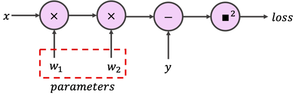
今回使用するモデルは、隠れ層が1つでニューロンも1つだけ、重みが2つのものです。コスト関数として二乗誤差（またはL2損失）を考えます。すでに想像がついているかもしれませんが、このモデルは以下のようにニューラルネットワークとして可視化できます：

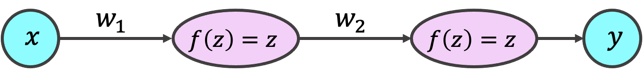
または計算グラフとして：

あるいは稀に、かなりコンパクトな写像としても表せます：

loss = (y - w_1 \cdot w_2 \cdot x)^2

自動微分ツールを使わずにニューラルネットワークを一から実装する必要はほとんどありません。したがって、以下の2つの演習はボーナス（任意）演習です。時間制限やプレッシャーがある場合は無視して、セクション1.2に進んでください。

解析演習 1.1: 損失の勾配（任意）

再度、次の演習で必要になるため、ネットワークの勾配を解析的に計算してください。面倒だと思いますがご理解ください。

$\dfrac{\partial{loss}}{\partial{w_1}} = ?$

$\dfrac{\partial{loss}}{\partial{w_2}} = ?$

解答

$\dfrac{\partial{loss}}{\partial{w_1}} = -2 \cdot w_2 \cdot x \cdot (y - w_1 \cdot w_2 \cdot x)$

$\dfrac{\partial{loss}}{\partial{w_2}} = -2 \cdot w_1 \cdot x \cdot (y - w_1 \cdot w_2 \cdot x)$

# @title Submit your feedback
content_review(f"{feedback_prefix}_Loss_Gradients_Analytical_Exercise")

コーディング演習 1.1: シンプルな狭いLNNの実装（任意）

次に、PyTorchを使わずにモデルの forward パスを一から実装してください。

また、モデルは単一の入力特徴量を受け取り単一の予測を出力しますが、複数のサンプルに対して一度に損失を計算しトレーニングを行うことも可能です。これはニューラルネットワークで一般的な手法であり、コンピュータは for ループでサンプルを一つずつ処理するよりも、バッチ単位での行列（またはテンソル）演算を非常に高速に行えるためです。したがって、loss 関数では平均二乗誤差（MSE）を実装し、dloss_dw 関数を実装する際には解析的勾配もそれに合わせて調整してください。

最後に、勾配降下法アルゴリズムのために train 関数を完成させてください：

\mathbf{w}^{(t+1)} = \mathbf{w}^{(t)} - \eta \nabla loss (\mathbf{w}^{(t)})

class ShallowNarrowExercise:
  """
  Shallow and narrow (one neuron per layer) linear neural network
  """

  def __init__(self, init_weights):
    """
    Initialize parameters of ShallowNarrow Net

    Args:
      init_weights: list
        Initial weights

    Returns:
      Nothing
    """
    assert isinstance(init_weights, (list, np.ndarray, tuple))
    assert len(init_weights) == 2
    self.w1 = init_weights[0]
    self.w2 = init_weights[1]


  def forward(self, x):
    """
    The forward pass through netwrok y = x * w1 * w2

    Args:
      x: np.ndarray
        Features (inputs) to neural net

    Returns:
      y: np.ndarray
        Neural network output (predictions)
    """
    #################################################
    ## Implement the forward pass to calculate prediction
    ## Note that prediction is not the loss
    # Complete the function and remove or comment the line below
    raise NotImplementedError("Forward Pass `forward`")
    #################################################
    y = ...
    return y


  def dloss_dw(self, x, y_true):
    """
    Gradient of loss with respect to weights

    Args:
      x: np.ndarray
        Features (inputs) to neural net
      y_true: np.ndarray
        True labels

    Returns:
      dloss_dw1: float
        Mean gradient of loss with respect to w1
      dloss_dw2: float
        Mean gradient of loss with respect to w2
    """
    assert x.shape == y_true.shape
    #################################################
    ## Implement the gradient computation function
    # Complete the function and remove or comment the line below
    raise NotImplementedError("Gradient of Loss `dloss_dw`")
    #################################################
    dloss_dw1 = ...
    dloss_dw2 = ...
    return dloss_dw1, dloss_dw2


  def train(self, x, y_true, lr, n_ep):
    """
    Training with Gradient descent algorithm

    Args:
      x: np.ndarray
        Features (inputs) to neural net
      y_true: np.ndarray
        True labels
      lr: float
        Learning rate
      n_ep: int
        Number of epochs (training iterations)

    Returns:
      loss_records: list
        Training loss records
      weight_records: list
        Training weight records (evolution of weights)
    """
    assert x.shape == y_true.shape

    loss_records = np.empty(n_ep)  # Pre allocation of loss records
    weight_records = np.empty((n_ep, 2))  # Pre allocation of weight records

    for i in range(n_ep):
      y_prediction = self.forward(x)
      loss_records[i] = loss(y_prediction, y_true)
      dloss_dw1, dloss_dw2 = self.dloss_dw(x, y_true)
      #################################################
      ## Implement the gradient descent step
      # Complete the function and remove or comment the line below
      raise NotImplementedError("Training loop `train`")
      #################################################
      self.w1 -= ...
      self.w2 -= ...
      weight_records[i] = [self.w1, self.w2]

    return loss_records, weight_records


def loss(y_prediction, y_true):
  """
  Mean squared error

  Args:
    y_prediction: np.ndarray
      Model output (prediction)
    y_true: np.ndarray
      True label

  Returns:
    mse: np.ndarray
      Mean squared error loss
  """
  assert y_prediction.shape == y_true.shape
  #################################################
  ## Implement the MEAN squared error
  # Complete the function and remove or comment the line below
  raise NotImplementedError("Loss function `loss`")
  #################################################
  mse = ...
  return mse



set_seed(seed=SEED)
n_epochs = 211
learning_rate = 0.02
initial_weights = [1.4, -1.6]
x_train, y_train = gen_samples(n=73, a=2.0, sigma=0.2)
x_eval = np.linspace(0.0, 1.0, 37, endpoint=True)
## Uncomment to run
# sn_model = ShallowNarrowExercise(initial_weights)
# loss_log, weight_log = sn_model.train(x_train, y_train, learning_rate, n_epochs)
# y_eval = sn_model.forward(x_eval)
# plot_x_y_(x_train, y_train, x_eval, y_eval, loss_log, weight_log)

解答を見る$

# @title Submit your feedback
content_review(f"{feedback_prefix}_Simple_Narrow_LNN_Exercise")

セクション 1.2: 学習の風景

# @title Video 2: Training Landscape
from ipywidgets import widgets
from IPython.display import YouTubeVideo
from IPython.display import IFrame
from IPython.display import display


class PlayVideo(IFrame):
  def __init__(self, id, source, page=1, width=400, height=300, **kwargs):
    self.id = id
    if source == 'Bilibili':
      src = f'https://player.bilibili.com/player.html?bvid={id}&page={page}'
    elif source == 'Osf':
      src = f'https://mfr.ca-1.osf.io/render?url=https://osf.io/download/{id}/?direct%26mode=render'
    super(PlayVideo, self).__init__(src, width, height, **kwargs)


def display_videos(video_ids, W=400, H=300, fs=1):
  tab_contents = []
  for i, video_id in enumerate(video_ids):
    out = widgets.Output()
    with out:
      if video_ids[i][0] == 'Youtube':
        video = YouTubeVideo(id=video_ids[i][1], width=W,
                             height=H, fs=fs, rel=0)
        print(f'Video available at https://youtube.com/watch?v={video.id}')
      else:
        video = PlayVideo(id=video_ids[i][1], source=video_ids[i][0], width=W,
                          height=H, fs=fs, autoplay=False)
        if video_ids[i][0] == 'Bilibili':
          print(f'Video available at https://www.bilibili.com/video/{video.id}')
        elif video_ids[i][0] == 'Osf':
          print(f'Video available at https://osf.io/{video.id}')
      display(video)
    tab_contents.append(out)
  return tab_contents


video_ids = [('Youtube', 'k28bnNAcOEg'), ('Bilibili', 'BV1Nv411J71X')]
tab_contents = display_videos(video_ids, W=854, H=480)
tabs = widgets.Tab()
tabs.children = tab_contents
for i in range(len(tab_contents)):
  tabs.set_title(i, video_ids[i][0])
display(tabs)

# @title Submit your feedback
content_review(f"{feedback_prefix}_Training_Landscape_Video")

すでに自分で考えたかもしれませんが、勾配降下法を使わずに解析的に $w_1$ と $w_2$ を求めることができます：

w_1 \cdot w_2 = \dfrac{y}{x}

実際に、勾配、損失関数、そしてすべての可能な解を一つの図にプロットできます。この例では、 $y = 1x$ の写像を使います：

青いリボン：すべての可能な解を示します： $~ w_1 w_2 = \dfrac{y}{x} = \dfrac{x}{x} = 1 \Rightarrow w_1 = \dfrac{1}{w_2}$

等高線の背景：損失値を示し、赤がより高い損失を表します

ベクトル場（矢印）：勾配ベクトル場を示します。大きな黄色の矢印は大きな勾配を示し、これは勾配降下法による大きなステップに対応します。

散布円：3つの異なる初期化における訓練中の重みの軌跡（変化）を示し、青い点が訓練開始を、赤いバツ（x）が訓練終了を示します。以下のように初期値を自分で試すこともできます（初期値は -2.0 から 2.0 の範囲にしてください）：

plot_vector_field('all', [1.0, -1.0])

最後に、プロットが込み合いすぎている場合は、以下の文字列のいずれかを引数として渡しても構いません：

plot_vector_field('vectors')  # ベクトル場用
plot_vector_field('trajectory')  # 訓練軌跡用
plot_vector_field('loss')  # 損失等高線用

考えてみましょう！

次の2つのプロットを探索し、異なる初期値を試してみてください。鞍点を見つけられますか？なぜ最小値付近で訓練が遅くなるのでしょうか？

plot_vector_field('all')

ここでは、損失ランドスケープを3Dプロットで可視化し、異なる初期条件に対する2つのトレーニング軌跡を示します。
注意：3Dプロットの軌跡と前のプロットの軌跡は独立しており、異なります。

plot_loss_landscape()

# @title Video 3: Training Landscape - Discussion
from ipywidgets import widgets
from IPython.display import YouTubeVideo
from IPython.display import IFrame
from IPython.display import display


class PlayVideo(IFrame):
  def __init__(self, id, source, page=1, width=400, height=300, **kwargs):
    self.id = id
    if source == 'Bilibili':
      src = f'https://player.bilibili.com/player.html?bvid={id}&page={page}'
    elif source == 'Osf':
      src = f'https://mfr.ca-1.osf.io/render?url=https://osf.io/download/{id}/?direct%26mode=render'
    super(PlayVideo, self).__init__(src, width, height, **kwargs)


def display_videos(video_ids, W=400, H=300, fs=1):
  tab_contents = []
  for i, video_id in enumerate(video_ids):
    out = widgets.Output()
    with out:
      if video_ids[i][0] == 'Youtube':
        video = YouTubeVideo(id=video_ids[i][1], width=W,
                             height=H, fs=fs, rel=0)
        print(f'Video available at https://youtube.com/watch?v={video.id}')
      else:
        video = PlayVideo(id=video_ids[i][1], source=video_ids[i][0], width=W,
                          height=H, fs=fs, autoplay=False)
        if video_ids[i][0] == 'Bilibili':
          print(f'Video available at https://www.bilibili.com/video/{video.id}')
        elif video_ids[i][0] == 'Osf':
          print(f'Video available at https://osf.io/{video.id}')
      display(video)
    tab_contents.append(out)
  return tab_contents


video_ids = [('Youtube', '0EcUGgxOdkI'), ('Bilibili', 'BV1py4y1j7cv')]
tab_contents = display_videos(video_ids, W=854, H=480)
tabs = widgets.Tab()
tabs.children = tab_contents
for i in range(len(tab_contents)):
  tabs.set_title(i, video_ids[i][0])
display(tabs)

# @title Submit your feedback
content_review(f"{feedback_prefix}_Training_Landscape_Discussion_Video")

セクション2：深さ、学習率、初期化

所要時間の目安：約45分

成功するディープラーニングモデルは、多くの場合、非常に優秀なチームが多くの時間をかけて学習のハイパーパラメータを「調整」し、効果的な初期化を見つけることで開発されます。このセクションでは、3つの基本的（しかししばしば単純ではない）なハイパーパラメータ、すなわち深さ、学習率、初期化について見ていきます。

セクション 2.1: 深さの効果

# @title Video 4: Effect of Depth
from ipywidgets import widgets
from IPython.display import YouTubeVideo
from IPython.display import IFrame
from IPython.display import display


class PlayVideo(IFrame):
  def __init__(self, id, source, page=1, width=400, height=300, **kwargs):
    self.id = id
    if source == 'Bilibili':
      src = f'https://player.bilibili.com/player.html?bvid={id}&page={page}'
    elif source == 'Osf':
      src = f'https://mfr.ca-1.osf.io/render?url=https://osf.io/download/{id}/?direct%26mode=render'
    super(PlayVideo, self).__init__(src, width, height, **kwargs)


def display_videos(video_ids, W=400, H=300, fs=1):
  tab_contents = []
  for i, video_id in enumerate(video_ids):
    out = widgets.Output()
    with out:
      if video_ids[i][0] == 'Youtube':
        video = YouTubeVideo(id=video_ids[i][1], width=W,
                             height=H, fs=fs, rel=0)
        print(f'Video available at https://youtube.com/watch?v={video.id}')
      else:
        video = PlayVideo(id=video_ids[i][1], source=video_ids[i][0], width=W,
                          height=H, fs=fs, autoplay=False)
        if video_ids[i][0] == 'Bilibili':
          print(f'Video available at https://www.bilibili.com/video/{video.id}')
        elif video_ids[i][0] == 'Osf':
          print(f'Video available at https://osf.io/{video.id}')
      display(video)
    tab_contents.append(out)
  return tab_contents


video_ids = [('Youtube', 'Ii_As9cRR5Q'), ('Bilibili', 'BV1z341167di')]
tab_contents = display_videos(video_ids, W=854, H=480)
tabs = widgets.Tab()
tabs.children = tab_contents
for i in range(len(tab_contents)):
  tabs.set_title(i, video_ids[i][0])
display(tabs)

# @title Submit your feedback
content_review(f"{feedback_prefix}_Effect_of_Depth_Video")

なぜ深さが役立つのでしょうか？ネットワークや学習システムを「深い」と呼ぶのはなぜでしょうか？実際のところ、浅いニューラルネットワークはデータの制約により複雑な関数を学習できないことが多いです。一方で、深さはまるで魔法のように感じられます。深さはネットワークが表現できる関数、ネットワークの学習方法、そして未知のデータに対する一般化の仕方を変えることができます。

では、深さがニューラルネットワークの訓練においてどのような課題をもたらすのか見てみましょう。単一入力・単一出力の線形ネットワークで、50層の隠れ層があり、各層に1つのニューロンしかない（つまり狭くて深いニューラルネットワーク）と想像してください。ネットワークの出力は簡単に計算できます：

prediction = x \cdot w_1 \cdot w_2 \cdot \cdot \cdot w_{50}

すべての重みの初期値が $w_i = 2$ の場合、 $x=1$ の予測は爆発的になります： $y_p = 2^{50} \approx 1.1256 \times 10^{15}$ 。一方、重みが $w_i = 0.5$ に初期化されている場合、出力は消失します： $y_p = 0.5^{50} \approx 8.88 \times 10^{-16}$ 。同様に、連鎖律を思い出すと、グラフが深くなるにつれて連鎖積の要素数が増え、勾配の爆発や消失につながる可能性があります。こうした数値的な脆弱性が訓練アルゴリズムを損なわないようにするために、深さの影響を理解する必要があります。

インタラクティブデモ 2.1: 深さウィジェット

ウィジェットを使って、深くて狭いニューラルネットワークの訓練曲線（損失の推移）に対する深さの影響を探ってみましょう。

考えてみよう！

どのネットワークが最も速く訓練されましたか？すべてのネットワークは最終的に「うまくいきましたか」（収束しましたか）？学習の軌跡はどのような形状でしたか？

# @markdown Make sure you execute this cell to enable the widget!

_ = interact(depth_widget,
    depth = IntSlider(min=0, max=51,
                      step=5, value=0,
                      continuous_update=False))

# @title Video 5: Effect of Depth - Discussion
from ipywidgets import widgets
from IPython.display import YouTubeVideo
from IPython.display import IFrame
from IPython.display import display


class PlayVideo(IFrame):
  def __init__(self, id, source, page=1, width=400, height=300, **kwargs):
    self.id = id
    if source == 'Bilibili':
      src = f'https://player.bilibili.com/player.html?bvid={id}&page={page}'
    elif source == 'Osf':
      src = f'https://mfr.ca-1.osf.io/render?url=https://osf.io/download/{id}/?direct%26mode=render'
    super(PlayVideo, self).__init__(src, width, height, **kwargs)


def display_videos(video_ids, W=400, H=300, fs=1):
  tab_contents = []
  for i, video_id in enumerate(video_ids):
    out = widgets.Output()
    with out:
      if video_ids[i][0] == 'Youtube':
        video = YouTubeVideo(id=video_ids[i][1], width=W,
                             height=H, fs=fs, rel=0)
        print(f'Video available at https://youtube.com/watch?v={video.id}')
      else:
        video = PlayVideo(id=video_ids[i][1], source=video_ids[i][0], width=W,
                          height=H, fs=fs, autoplay=False)
        if video_ids[i][0] == 'Bilibili':
          print(f'Video available at https://www.bilibili.com/video/{video.id}')
        elif video_ids[i][0] == 'Osf':
          print(f'Video available at https://osf.io/{video.id}')
      display(video)
    tab_contents.append(out)
  return tab_contents


video_ids = [('Youtube', 'EqSDkwmSruk'), ('Bilibili', 'BV1Qq4y1H7uk')]
tab_contents = display_videos(video_ids, W=854, H=480)
tabs = widgets.Tab()
tabs.children = tab_contents
for i in range(len(tab_contents)):
  tabs.set_title(i, video_ids[i][0])
display(tabs)

# @title Submit your feedback
content_review(f"{feedback_prefix}_Effect_of_Depth_Discussion_Video")

セクション 2.2: 学習率の選択

学習率はほとんどの最適化アルゴリズムで共通のハイパーパラメータです。どのように設定すべきでしょうか？時にはすべての可能性を試すしかありませんが、時にはいくつかの重要なトレードオフを知っていることで良いハイパーパラメータ探索の指針になります。

# @title Video 6: Learning Rate
from ipywidgets import widgets
from IPython.display import YouTubeVideo
from IPython.display import IFrame
from IPython.display import display


class PlayVideo(IFrame):
  def __init__(self, id, source, page=1, width=400, height=300, **kwargs):
    self.id = id
    if source == 'Bilibili':
      src = f'https://player.bilibili.com/player.html?bvid={id}&page={page}'
    elif source == 'Osf':
      src = f'https://mfr.ca-1.osf.io/render?url=https://osf.io/download/{id}/?direct%26mode=render'
    super(PlayVideo, self).__init__(src, width, height, **kwargs)


def display_videos(video_ids, W=400, H=300, fs=1):
  tab_contents = []
  for i, video_id in enumerate(video_ids):
    out = widgets.Output()
    with out:
      if video_ids[i][0] == 'Youtube':
        video = YouTubeVideo(id=video_ids[i][1], width=W,
                             height=H, fs=fs, rel=0)
        print(f'Video available at https://youtube.com/watch?v={video.id}')
      else:
        video = PlayVideo(id=video_ids[i][1], source=video_ids[i][0], width=W,
                          height=H, fs=fs, autoplay=False)
        if video_ids[i][0] == 'Bilibili':
          print(f'Video available at https://www.bilibili.com/video/{video.id}')
        elif video_ids[i][0] == 'Osf':
          print(f'Video available at https://osf.io/{video.id}')
      display(video)
    tab_contents.append(out)
  return tab_contents


video_ids = [('Youtube', 'w_GrCVM-_Qo'), ('Bilibili', 'BV11f4y157MT')]
tab_contents = display_videos(video_ids, W=854, H=480)
tabs = widgets.Tab()
tabs.children = tab_contents
for i in range(len(tab_contents)):
  tabs.set_title(i, video_ids[i][0])
display(tabs)

# @title Submit your feedback
content_review(f"{feedback_prefix}_Learning_Rate_Video")

インタラクティブデモ 2.2: 学習率ウィジェット

ここではネットワークの深さを50層に固定しています。ウィジェットを使って、深くて狭いニューラルネットワークの訓練曲線（損失の推移）に対する学習率 $\eta$ の影響を探ってみましょう。

考えてみよう！

学習率が大きいほど常に学習が速くなると言えるでしょうか？なぜそうではないのでしょうか？

# @markdown Make sure you execute this cell to enable the widget!

_ = interact(lr_widget,
    lr = FloatSlider(min=0.005, max=0.045, step=0.005, value=0.005,
                     continuous_update=False, readout_format='.3f',
                     description='eta'))

# @title Video 7: Learning Rate - Discussion
from ipywidgets import widgets
from IPython.display import YouTubeVideo
from IPython.display import IFrame
from IPython.display import display


class PlayVideo(IFrame):
  def __init__(self, id, source, page=1, width=400, height=300, **kwargs):
    self.id = id
    if source == 'Bilibili':
      src = f'https://player.bilibili.com/player.html?bvid={id}&page={page}'
    elif source == 'Osf':
      src = f'https://mfr.ca-1.osf.io/render?url=https://osf.io/download/{id}/?direct%26mode=render'
    super(PlayVideo, self).__init__(src, width, height, **kwargs)


def display_videos(video_ids, W=400, H=300, fs=1):
  tab_contents = []
  for i, video_id in enumerate(video_ids):
    out = widgets.Output()
    with out:
      if video_ids[i][0] == 'Youtube':
        video = YouTubeVideo(id=video_ids[i][1], width=W,
                             height=H, fs=fs, rel=0)
        print(f'Video available at https://youtube.com/watch?v={video.id}')
      else:
        video = PlayVideo(id=video_ids[i][1], source=video_ids[i][0], width=W,
                          height=H, fs=fs, autoplay=False)
        if video_ids[i][0] == 'Bilibili':
          print(f'Video available at https://www.bilibili.com/video/{video.id}')
        elif video_ids[i][0] == 'Osf':
          print(f'Video available at https://osf.io/{video.id}')
      display(video)
    tab_contents.append(out)
  return tab_contents


video_ids = [('Youtube', 'cmS0yqImz2E'), ('Bilibili', 'BV1Aq4y1p7bh')]
tab_contents = display_videos(video_ids, W=854, H=480)
tabs = widgets.Tab()
tabs.children = tab_contents
for i in range(len(tab_contents)):
  tabs.set_title(i, video_ids[i][0])
display(tabs)

# @title Submit your feedback
content_review(f"{feedback_prefix}_Learning_Rate_Discussion_Video")

セクション 2.3: 深さと学習率

# @title Video 8: Depth and Learning Rate
from ipywidgets import widgets
from IPython.display import YouTubeVideo
from IPython.display import IFrame
from IPython.display import display


class PlayVideo(IFrame):
  def __init__(self, id, source, page=1, width=400, height=300, **kwargs):
    self.id = id
    if source == 'Bilibili':
      src = f'https://player.bilibili.com/player.html?bvid={id}&page={page}'
    elif source == 'Osf':
      src = f'https://mfr.ca-1.osf.io/render?url=https://osf.io/download/{id}/?direct%26mode=render'
    super(PlayVideo, self).__init__(src, width, height, **kwargs)


def display_videos(video_ids, W=400, H=300, fs=1):
  tab_contents = []
  for i, video_id in enumerate(video_ids):
    out = widgets.Output()
    with out:
      if video_ids[i][0] == 'Youtube':
        video = YouTubeVideo(id=video_ids[i][1], width=W,
                             height=H, fs=fs, rel=0)
        print(f'Video available at https://youtube.com/watch?v={video.id}')
      else:
        video = PlayVideo(id=video_ids[i][1], source=video_ids[i][0], width=W,
                          height=H, fs=fs, autoplay=False)
        if video_ids[i][0] == 'Bilibili':
          print(f'Video available at https://www.bilibili.com/video/{video.id}')
        elif video_ids[i][0] == 'Osf':
          print(f'Video available at https://osf.io/{video.id}')
      display(video)
    tab_contents.append(out)
  return tab_contents


video_ids = [('Youtube', 'J30phrux_3k'), ('Bilibili', 'BV1V44y1177e')]
tab_contents = display_videos(video_ids, W=854, H=480)
tabs = widgets.Tab()
tabs.children = tab_contents
for i in range(len(tab_contents)):
  tabs.set_title(i, video_ids[i][0])
display(tabs)

# @title Submit your feedback
content_review(f"{feedback_prefix}_Depth_and_Learning_Rate_Video")

インタラクティブデモ 2.3: 深さと学習率

重要な指示
演習は10層の隠れ層から始まります。あなたの課題は、速くかつ安定した収束（学習）をもたらす学習率を見つけることです。学習率に自信が持てたら、その深さに対して最適な学習率を登録できます。登録ボタンを押すとより深いモデルが生成され、次の最適な学習率を見つけることができます。登録ボタンは訓練が収束したときにのみ緑色になりますが、最速の収束を意味するわけではありません。最後に、ウィジェットは動作が遅いので気長にお待ちください。

考えてみよう！

深さと最適な学習率の関係を説明できますか？

# @markdown Make sure you execute this cell to enable the widget!
intpl_obj = InterPlay()

intpl_obj.slider = FloatSlider(min=0.005, max=0.105, step=0.005, value=0.005,
                               layout=Layout(width='500px'),
                               continuous_update=False,
                               readout_format='.3f',
                               description='eta')

intpl_obj.button = ToggleButton(value=intpl_obj.converged, description='Register')

widgets_ui = HBox([intpl_obj.slider, intpl_obj.button])
widgets_out = interactive_output(intpl_obj.train,
                                 {'lr': intpl_obj.slider,
                                  'update': intpl_obj.button,
                                  'init_weights': fixed(0.9)})

display(widgets_ui, widgets_out)

# @title Submit your feedback
content_review(f"{feedback_prefix}_Depth_and_Learning_Rate_Interactive_Demo")

# @title Video 9: Depth and Learning Rate - Discussion
from ipywidgets import widgets
from IPython.display import YouTubeVideo
from IPython.display import IFrame
from IPython.display import display


class PlayVideo(IFrame):
  def __init__(self, id, source, page=1, width=400, height=300, **kwargs):
    self.id = id
    if source == 'Bilibili':
      src = f'https://player.bilibili.com/player.html?bvid={id}&page={page}'
    elif source == 'Osf':
      src = f'https://mfr.ca-1.osf.io/render?url=https://osf.io/download/{id}/?direct%26mode=render'
    super(PlayVideo, self).__init__(src, width, height, **kwargs)


def display_videos(video_ids, W=400, H=300, fs=1):
  tab_contents = []
  for i, video_id in enumerate(video_ids):
    out = widgets.Output()
    with out:
      if video_ids[i][0] == 'Youtube':
        video = YouTubeVideo(id=video_ids[i][1], width=W,
                             height=H, fs=fs, rel=0)
        print(f'Video available at https://youtube.com/watch?v={video.id}')
      else:
        video = PlayVideo(id=video_ids[i][1], source=video_ids[i][0], width=W,
                          height=H, fs=fs, autoplay=False)
        if video_ids[i][0] == 'Bilibili':
          print(f'Video available at https://www.bilibili.com/video/{video.id}')
        elif video_ids[i][0] == 'Osf':
          print(f'Video available at https://osf.io/{video.id}')
      display(video)
    tab_contents.append(out)
  return tab_contents


video_ids = [('Youtube', '7Fl8vH7cgco'), ('Bilibili', 'BV15q4y1p7Uq')]
tab_contents = display_videos(video_ids, W=854, H=480)
tabs = widgets.Tab()
tabs.children = tab_contents
for i in range(len(tab_contents)):
  tabs.set_title(i, video_ids[i][0])
display(tabs)

# @title Submit your feedback
content_review(f"{feedback_prefix}_Depth_and_Learning_Rate_Discussion_Video")

セクション 2.4: なぜ初期化が重要なのか

# @title Video 10: Initialization Matters
from ipywidgets import widgets
from IPython.display import YouTubeVideo
from IPython.display import IFrame
from IPython.display import display


class PlayVideo(IFrame):
  def __init__(self, id, source, page=1, width=400, height=300, **kwargs):
    self.id = id
    if source == 'Bilibili':
      src = f'https://player.bilibili.com/player.html?bvid={id}&page={page}'
    elif source == 'Osf':
      src = f'https://mfr.ca-1.osf.io/render?url=https://osf.io/download/{id}/?direct%26mode=render'
    super(PlayVideo, self).__init__(src, width, height, **kwargs)


def display_videos(video_ids, W=400, H=300, fs=1):
  tab_contents = []
  for i, video_id in enumerate(video_ids):
    out = widgets.Output()
    with out:
      if video_ids[i][0] == 'Youtube':
        video = YouTubeVideo(id=video_ids[i][1], width=W,
                             height=H, fs=fs, rel=0)
        print(f'Video available at https://youtube.com/watch?v={video.id}')
      else:
        video = PlayVideo(id=video_ids[i][1], source=video_ids[i][0], width=W,
                          height=H, fs=fs, autoplay=False)
        if video_ids[i][0] == 'Bilibili':
          print(f'Video available at https://www.bilibili.com/video/{video.id}')
        elif video_ids[i][0] == 'Osf':
          print(f'Video available at https://osf.io/{video.id}')
      display(video)
    tab_contents.append(out)
  return tab_contents


video_ids = [('Youtube', 'KmqCz95AMzY'), ('Bilibili', 'BV1UL411J7vu')]
tab_contents = display_videos(video_ids, W=854, H=480)
tabs = widgets.Tab()
tabs.children = tab_contents
for i in range(len(tab_contents)):
  tabs.set_title(i, video_ids[i][0])
display(tabs)

# @title Submit your feedback
content_review(f"{feedback_prefix}_Initialization_Matters")

最も単純な場合でも、深さが学習を遅くすることがあると見てきました。なぜでしょうか？連鎖律から、勾配は各層の現在の重みによって掛け合わされるため、積が消失したり爆発したりする可能性があります。したがって、重みの初期化は根本的に重要なハイパーパラメータです。

実際には学習可能なパラメータの初期値は様々な $\mathcal{Uniform}$ や $\mathcal{Normal}$ 確率分布からサンプリングされることが多いですが、ここではすべてのパラメータに単一の値を使っています。

下の図は、深くて狭い線形ニューラルネットワークにおける初期化が学習速度に与える影響を示しています。nan や inf といった数値エラーを引き起こすような初期化（小さすぎたり大きすぎたりするもの）は除外しています。

# @markdown Make sure you execute this cell to see the figure!

plot_init_effect()

# @title Video 11: Initialization Matters - Discussion
from ipywidgets import widgets
from IPython.display import YouTubeVideo
from IPython.display import IFrame
from IPython.display import display


class PlayVideo(IFrame):
  def __init__(self, id, source, page=1, width=400, height=300, **kwargs):
    self.id = id
    if source == 'Bilibili':
      src = f'https://player.bilibili.com/player.html?bvid={id}&page={page}'
    elif source == 'Osf':
      src = f'https://mfr.ca-1.osf.io/render?url=https://osf.io/download/{id}/?direct%26mode=render'
    super(PlayVideo, self).__init__(src, width, height, **kwargs)


def display_videos(video_ids, W=400, H=300, fs=1):
  tab_contents = []
  for i, video_id in enumerate(video_ids):
    out = widgets.Output()
    with out:
      if video_ids[i][0] == 'Youtube':
        video = YouTubeVideo(id=video_ids[i][1], width=W,
                             height=H, fs=fs, rel=0)
        print(f'Video available at https://youtube.com/watch?v={video.id}')
      else:
        video = PlayVideo(id=video_ids[i][1], source=video_ids[i][0], width=W,
                          height=H, fs=fs, autoplay=False)
        if video_ids[i][0] == 'Bilibili':
          print(f'Video available at https://www.bilibili.com/video/{video.id}')
        elif video_ids[i][0] == 'Osf':
          print(f'Video available at https://osf.io/{video.id}')
      display(video)
    tab_contents.append(out)
  return tab_contents


video_ids = [('Youtube', 'vKktGdiQDsE'), ('Bilibili', 'BV1hM4y1T7gJ')]
tab_contents = display_videos(video_ids, W=854, H=480)
tabs = widgets.Tab()
tabs.children = tab_contents
for i in range(len(tab_contents)):
  tabs.set_title(i, video_ids[i][0])
display(tabs)

# @title Submit your feedback
content_review(f"{feedback_prefix}_Initialization_Matters_Discussion_Video")

まとめ

第2回のチュートリアルでは、訓練のランドスケープとは何かを学び、ネットワークの深さと学習率の効果およびそれらの相互作用を詳しく見てきました。最後に、初期化が重要である理由と賢い初期化方法の必要性についても理解しました。

# @title Video 12: Tutorial 2 Wrap-up
from ipywidgets import widgets
from IPython.display import YouTubeVideo
from IPython.display import IFrame
from IPython.display import display


class PlayVideo(IFrame):
  def __init__(self, id, source, page=1, width=400, height=300, **kwargs):
    self.id = id
    if source == 'Bilibili':
      src = f'https://player.bilibili.com/player.html?bvid={id}&page={page}'
    elif source == 'Osf':
      src = f'https://mfr.ca-1.osf.io/render?url=https://osf.io/download/{id}/?direct%26mode=render'
    super(PlayVideo, self).__init__(src, width, height, **kwargs)


def display_videos(video_ids, W=400, H=300, fs=1):
  tab_contents = []
  for i, video_id in enumerate(video_ids):
    out = widgets.Output()
    with out:
      if video_ids[i][0] == 'Youtube':
        video = YouTubeVideo(id=video_ids[i][1], width=W,
                             height=H, fs=fs, rel=0)
        print(f'Video available at https://youtube.com/watch?v={video.id}')
      else:
        video = PlayVideo(id=video_ids[i][1], source=video_ids[i][0], width=W,
                          height=H, fs=fs, autoplay=False)
        if video_ids[i][0] == 'Bilibili':
          print(f'Video available at https://www.bilibili.com/video/{video.id}')
        elif video_ids[i][0] == 'Osf':
          print(f'Video available at https://osf.io/{video.id}')
      display(video)
    tab_contents.append(out)
  return tab_contents


video_ids = [('Youtube', 'r3K8gtak3wA'), ('Bilibili', 'BV1P44y117Pd')]
tab_contents = display_videos(video_ids, W=854, H=480)
tabs = widgets.Tab()
tabs.children = tab_contents
for i in range(len(tab_contents)):
  tabs.set_title(i, video_ids[i][0])
display(tabs)

# @title Submit your feedback
content_review(f"{feedback_prefix}_WrapUp_Video")

ボーナス

ハイパーパラメータの相互作用

最後に、これまで学んだことをすべてまとめて、与えられた深さに対して最適な初期重みと学習率を見つけましょう。これまでの学習で相互作用を理解し、最適な値を素早く見つける方法を身につけているはずです。もし 数値オーバーフロー の警告が出ても落胆しないでください！それらは多くの場合「勾配の爆発」や「消失」が原因です。

考えてみよう！

驚くような挙動や最適なパラメータを見つけるのに苦労したことはありましたか？

# @markdown Make sure you execute this cell to enable the widget!

_ = interact(depth_lr_init_interplay,
             depth = IntSlider(min=10, max=51, step=5, value=25,
                               continuous_update=False),
             lr = FloatSlider(min=0.001, max=0.1,
                              step=0.005, value=0.005,
                              continuous_update=False,
                              readout_format='.3f',
                              description='eta'),
             init_weights = FloatSlider(min=0.1, max=3.0,
                                        step=0.1, value=0.9,
                                        continuous_update=False,
                                        readout_format='.3f',
                                        description='initial weights'))

# @title Submit your feedback
content_review(f"{feedback_prefix}_Hyperparameter_interaction_Bonus_Discussion")