![]()

チュートリアル 1: 勾配降下法とAutoGrad
第1週、第2日目:線形ディープラーニング
Neuromatch Academyによる
コンテンツ作成者: Saeed Salehi, Vladimir Haltakov, Andrew Saxe
コンテンツレビュアー: Polina Turishcheva, Antoine De Comite, Kelson Shilling-Scrivo
コンテンツ編集者: Anoop Kulkarni, Spiros Chavlis
制作編集者: Khalid Almubarak, Gagana B, Spiros Chavlis
チュートリアルの目的
第2日目のチュートリアル1では、PyTorchのスキルセット構築を続け、その中核機能であるAutogradを動機付けます。このノートブックでは、以下の重要な概念とアイデアを扱います:
- 勾配降下法
- PyTorchのAutograd
- PyTorchの
nnモジュール
# @title Tutorial slides
from IPython.display import IFrame
link_id = "3qevp"
print(f"If you want to download the slides: https://osf.io/download/{link_id}/")
IFrame(src=f"https://mfr.ca-1.osf.io/render?url=https://osf.io/{link_id}/?direct%26mode=render%26action=download%26mode=render", width=854, height=480)
セットアップ
このチュートリアルはGPU不要です!
# @title Install and import feedback gadget


from vibecheck import DatatopsContentReviewContainer
def content_review(notebook_section: str):
    return DatatopsContentReviewContainer(
        "",  # No text prompt
        notebook_section,
        {
            "url": "https://pmyvdlilci.execute-api.us-east-1.amazonaws.com/klab",
            "name": "neuromatch_dl",
            "user_key": "f379rz8y",
        },
    ).render()


feedback_prefix = "W1D2_T1"
# Imports
import torch
import numpy as np
from torch import nn
from math import pi
import matplotlib.pyplot as plt# @title Figure settings
import logging
logging.getLogger('matplotlib.font_manager').disabled = True
import ipywidgets as widgets # Interactive display
%config InlineBackend.figure_format = 'retina'
plt.style.use("https://raw.githubusercontent.com/NeuromatchAcademy/content-creation/main/nma.mplstyle")# @title Plotting functions
from mpl_toolkits.axes_grid1 import make_axes_locatable
def ex3_plot(model, x, y, ep, lss):
"""
Plot training loss
Args:
model: nn.module
Model implementing regression
x: np.ndarray
Training Data
y: np.ndarray
Targets
ep: int
Number of epochs
lss: function
Loss function
Returns:
Nothing
"""
f, (ax1, ax2) = plt.subplots(1, 2, figsize=(12, 4))
ax1.set_title("Regression")
ax1.plot(x, model(x).detach().numpy(), color='r', label='prediction')
ax1.scatter(x, y, c='c', label='targets')
ax1.set_xlabel('x')
ax1.set_ylabel('y')
ax1.legend()
ax2.set_title("Training loss")
ax2.plot(np.linspace(1, epochs, epochs), losses, color='y')
ax2.set_xlabel("Epoch")
ax2.set_ylabel("MSE")
plt.show()
def ex1_plot(fun_z, fun_dz):
"""
Plots the function and gradient vectors
Args:
fun_z: f.__name__
Function implementing sine function
fun_dz: f.__name__
Function implementing sine function as gradient vector
Returns:
Nothing
"""
x, y = np.arange(-3, 3.01, 0.02), np.arange(-3, 3.01, 0.02)
xx, yy = np.meshgrid(x, y, sparse=True)
zz = fun_z(xx, yy)
xg, yg = np.arange(-2.5, 2.6, 0.5), np.arange(-2.5, 2.6, 0.5)
xxg, yyg = np.meshgrid(xg, yg, sparse=True)
zxg, zyg = fun_dz(xxg, yyg)
plt.figure(figsize=(8, 7))
plt.title("Gradient vectors point towards steepest ascent")
contplt = plt.contourf(x, y, zz, levels=20)
plt.quiver(xxg, yyg, zxg, zyg, scale=50, color='r', )
plt.xlabel('$x$')
plt.ylabel('$y$')
ax = plt.gca()
divider = make_axes_locatable(ax)
cax = divider.append_axes("right", size="5%", pad=0.05)
cbar = plt.colorbar(contplt, cax=cax)
cbar.set_label('$z = h(x, y)$')
plt.show()# @title Set random seed
# @markdown Executing `set_seed(seed=seed)` you are setting the seed
# For DL its critical to set the random seed so that students can have a
# baseline to compare their results to expected results.
# Read more here: https://pytorch.org/docs/stable/notes/randomness.html
# Call `set_seed` function in the exercises to ensure reproducibility.
import random
import torch
def set_seed(seed=None, seed_torch=True):
"""
Function that controls randomness. NumPy and random modules must be imported.
Args:
seed : Integer
A non-negative integer that defines the random state. Default is `None`.
seed_torch : Boolean
If `True` sets the random seed for pytorch tensors, so pytorch module
must be imported. Default is `True`.
Returns:
Nothing.
"""
if seed is None:
seed = np.random.choice(2 ** 32)
random.seed(seed)
np.random.seed(seed)
if seed_torch:
torch.manual_seed(seed)
torch.cuda.manual_seed_all(seed)
torch.cuda.manual_seed(seed)
torch.backends.cudnn.benchmark = False
torch.backends.cudnn.deterministic = True
print(f'Random seed {seed} has been set.')
# In case that `DataLoader` is used
def seed_worker(worker_id):
"""
DataLoader will reseed workers following randomness in
multi-process data loading algorithm.
Args:
worker_id: integer
ID of subprocess to seed. 0 means that
the data will be loaded in the main process
Refer: https://pytorch.org/docs/stable/data.html#data-loading-randomness for more details
Returns:
Nothing
"""
worker_seed = torch.initial_seed() % 2**32
np.random.seed(worker_seed)
random.seed(worker_seed)# @title Set device (GPU or CPU). Execute `set_device()`
# especially if torch modules used.
# inform the user if the notebook uses GPU or CPU.
def set_device():
"""
Set the device. CUDA if available, CPU otherwise
Args:
None
Returns:
Nothing
"""
device = "cuda" if torch.cuda.is_available() else "cpu"
if device != "cuda":
print("GPU is not enabled in this notebook. \n"
"If you want to enable it, in the menu under `Runtime` -> \n"
"`Hardware accelerator.` and select `GPU` from the dropdown menu")
else:
print("GPU is enabled in this notebook. \n"
"If you want to disable it, in the menu under `Runtime` -> \n"
"`Hardware accelerator.` and select `None` from the dropdown menu")
return deviceSEED = 2021
set_seed(seed=SEED)
DEVICE = set_device()セクション0: はじめに
本日は3つのチュートリアルを進めます。
- まずはディープラーニングアルゴリズムの主力である勾配降下法から始めます。
- 2つ目のチュートリアルでは、ニューラルネットワークと基本的なハイパーパラメータについての直感を深めます。
- 最後に、チュートリアル3では学習のダイナミクス、良い深層ネットワークが何を学習しているか、そして時に性能が悪くなる理由を学びます。
# @title Video 0: Introduction
from ipywidgets import widgets
from IPython.display import YouTubeVideo
from IPython.display import IFrame
from IPython.display import display


class PlayVideo(IFrame):
  def __init__(self, id, source, page=1, width=400, height=300, **kwargs):
    self.id = id
    if source == 'Bilibili':
      src = f'https://player.bilibili.com/player.html?bvid={id}&page={page}'
    elif source == 'Osf':
      src = f'https://mfr.ca-1.osf.io/render?url=https://osf.io/download/{id}/?direct%26mode=render'
    super(PlayVideo, self).__init__(src, width, height, **kwargs)


def display_videos(video_ids, W=400, H=300, fs=1):
  tab_contents = []
  for i, video_id in enumerate(video_ids):
    out = widgets.Output()
    with out:
      if video_ids[i][0] == 'Youtube':
        video = YouTubeVideo(id=video_ids[i][1], width=W,
                             height=H, fs=fs, rel=0)
        print(f'Video available at https://youtube.com/watch?v={video.id}')
      else:
        video = PlayVideo(id=video_ids[i][1], source=video_ids[i][0], width=W,
                          height=H, fs=fs, autoplay=False)
        if video_ids[i][0] == 'Bilibili':
          print(f'Video available at https://www.bilibili.com/video/{video.id}')
        elif video_ids[i][0] == 'Osf':
          print(f'Video available at https://osf.io/{video.id}')
      display(video)
    tab_contents.append(out)
  return tab_contents


video_ids = [('Youtube', 'i7djAv2jnzY'), ('Bilibili', 'BV1Qf4y1578t')]
tab_contents = display_videos(video_ids, W=854, H=480)
tabs = widgets.Tab()
tabs.children = tab_contents
for i in range(len(tab_contents)):
  tabs.set_title(i, video_ids[i][0])
display(tabs)
# @title Submit your feedback
content_review(f"{feedback_prefix}_Introduction_Video")セクション1: 勾配降下法アルゴリズム
所要時間の目安:約30~45分
ほとんどの学習アルゴリズムの目標はリスク(コストまたは損失関数とも呼ばれる)を最小化することであり、最適化は多くの機械学習技術の核心です!勾配降下法アルゴリズムは、確率的勾配降下法などの変種とともに、ディープラーニングで最も強力かつ人気のある最適化手法の一つです。本日は基本を紹介しますが、最適化については今後(第1週、第4日目)さらに学びます。
セクション1.1: 勾配と最急上昇方向
# @title Video 1: Gradient Descent
from ipywidgets import widgets
from IPython.display import YouTubeVideo
from IPython.display import IFrame
from IPython.display import display


class PlayVideo(IFrame):
  def __init__(self, id, source, page=1, width=400, height=300, **kwargs):
    self.id = id
    if source == 'Bilibili':
      src = f'https://player.bilibili.com/player.html?bvid={id}&page={page}'
    elif source == 'Osf':
      src = f'https://mfr.ca-1.osf.io/render?url=https://osf.io/download/{id}/?direct%26mode=render'
    super(PlayVideo, self).__init__(src, width, height, **kwargs)


def display_videos(video_ids, W=400, H=300, fs=1):
  tab_contents = []
  for i, video_id in enumerate(video_ids):
    out = widgets.Output()
    with out:
      if video_ids[i][0] == 'Youtube':
        video = YouTubeVideo(id=video_ids[i][1], width=W,
                             height=H, fs=fs, rel=0)
        print(f'Video available at https://youtube.com/watch?v={video.id}')
      else:
        video = PlayVideo(id=video_ids[i][1], source=video_ids[i][0], width=W,
                          height=H, fs=fs, autoplay=False)
        if video_ids[i][0] == 'Bilibili':
          print(f'Video available at https://www.bilibili.com/video/{video.id}')
        elif video_ids[i][0] == 'Osf':
          print(f'Video available at https://osf.io/{video.id}')
      display(video)
    tab_contents.append(out)
  return tab_contents


video_ids = [('Youtube', 'UwgA_SgG0TM'), ('Bilibili', 'BV1Pq4y1p7em')]
tab_contents = display_videos(video_ids, W=854, H=480)
tabs = widgets.Tab()
tabs.children = tab_contents
for i in range(len(tab_contents)):
  tabs.set_title(i, video_ids[i][0])
display(tabs)
# @title Submit your feedback
content_review(f"{feedback_prefix}_Gradient_Descent_Video")勾配降下法アルゴリズムを紹介する前に、勾配の非常に重要な性質を復習しましょう。関数の勾配は常に最も急な上昇方向を指します。以下の演習でこれを明確にします。
演習1.1: 勾配ベクトル(任意)
次の関数が与えられています:
勾配ベクトルを求めなさい:
ヒント:連鎖律を使いましょう!
連鎖律:合成関数 に対して:
または別の表記で:
解答を見るにはここをクリック
関数を合成関数として書き換えます:
連鎖律$を使うと:
\begin{align}
&= ~ (2x) = \ \
&= ~ (2y) = \cos(x^2 + y^2) \cdot 2y
\end{align}
# @title Submit your feedback
content_review(f"{feedback_prefix}_Gradient_Vector_Analytical_Exercise")
コーディング演習1.1: 勾配ベクトル
関数 の勾配ベクトルを返す関数を実装(完成)してください。
def fun_z(x, y):
  """
  Implements function sin(x^2 + y^2)

  Args:
    x: (float, np.ndarray)
      Variable x
    y: (float, np.ndarray)
      Variable y

  Returns:
    z: (float, np.ndarray)
      sin(x^2 + y^2)
  """
  z = np.sin(x**2 + y**2)
  return z


def fun_dz(x, y):
  """
  Implements function sin(x^2 + y^2)

  Args:
    x: (float, np.ndarray)
      Variable x
    y: (float, np.ndarray)
      Variable y

  Returns:
    Tuple of gradient vector for sin(x^2 + y^2)
  """
  #################################################
  ## Implement the function which returns gradient vector
  ## Complete the partial derivatives dz_dx and dz_dy
  # Complete the function and remove or comment the line below
  raise NotImplementedError("Gradient function `fun_dz`")
  #################################################
  dz_dx = ...
  dz_dy = ...
  return (dz_dx, dz_dy)


## Uncomment to run
# ex1_plot(fun_z, fun_dz)出力例:
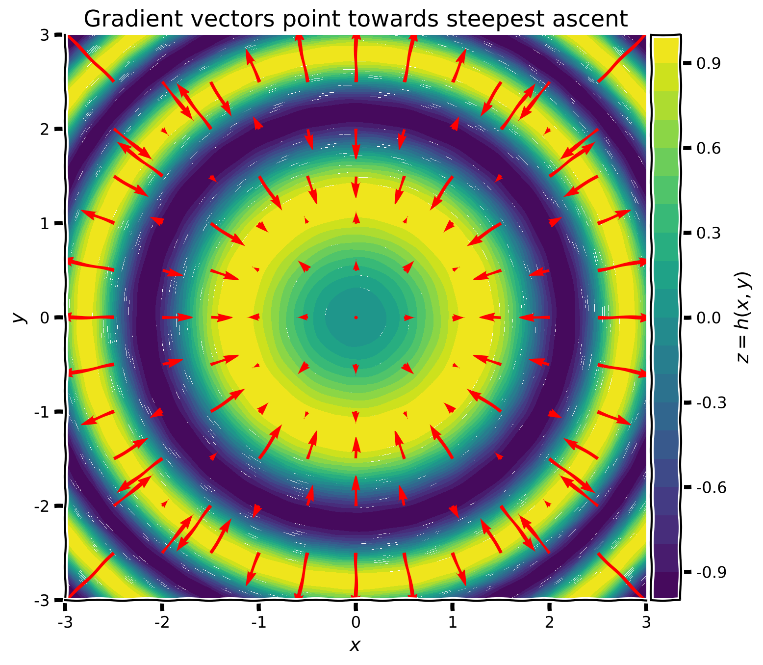
プロットからわかるように、任意の点 において、勾配ベクトル は が最も増加する方向を指します。勾配ベクトルは局所的な値のみを見ており、関数全体の形状を把握しているわけではありません。また、各ベクトルの長さ(大きさ)は関数の傾斜の急さを示し、局所的な平坦な領域(例えば極小値や極大値付近)では非常に小さくなることがあります。
したがって、上述の式を使って局所最小値を見つけることができます。
1847年、Augustin-Louis Cauchyは勾配の負の方向を用いて、多変数の連続かつ(理想的には)微分可能な関数を反復的に****最小化する勾配降下法アルゴリズムを開発しました。
# @title Submit your feedback
content_review(f"{feedback_prefix}_Gradient_Vector_Exercise")
# @title Video 2: Gradient Descent - Discussion
from ipywidgets import widgets
from IPython.display import YouTubeVideo
from IPython.display import IFrame
from IPython.display import display
class PlayVideo(IFrame):
def __init__(self, id, source, page=1, width=400, height=300, **kwargs):
self.id = id
if source == 'Bilibili':
src = f'https://player.bilibili.com/player.html?bvid={id}&page={page}'
elif source == 'Osf':
src = f'https://mfr.ca-1.osf.io/render?url=https://osf.io/download/{id}/?direct%26mode=render'
super(PlayVideo, self).__init__(src, width, height, **kwargs)
def display_videos(video_ids, W=400, H=300, fs=1):
tab_contents = []
for i, video_id in enumerate(video_ids):
out = widgets.Output()
with out:
if video_ids[i][0] == 'Youtube':
video = YouTubeVideo(id=video_ids[i][1], width=W,
height=H, fs=fs, rel=0)
print(f'Video available at https://youtube.com/watch?v={video.id}')
else:
video = PlayVideo(id=video_ids[i][1], source=video_ids[i][0], width=W,
height=H, fs=fs, autoplay=False)
if video_ids[i][0] == 'Bilibili':
print(f'Video available at https://www.bilibili.com/video/{video.id}')
elif video_ids[i][0] == 'Osf':
print(f'Video available at https://osf.io/{video.id}')
display(video)
tab_contents.append(out)
return tab_contents
video_ids = [('Youtube', '8s22ffAfGwI'), ('Bilibili', 'BV1Rf4y157bw')]
tab_contents = display_videos(video_ids, W=854, H=480)
tabs = widgets.Tab()
tabs.children = tab_contents
for i in range(len(tab_contents)):
tabs.set_title(i, video_ids[i][0])
display(tabs)# @title Submit your feedback
content_review(f"{feedback_prefix}_Gradient_Descent_Discussion_Video")セクション1.2: 勾配降下法アルゴリズム
を微分可能な関数とします。勾配降下法は、変数 の初期値から始めて、現在の点での勾配の負の方向に学習率 の大きさのステップを踏みながら関数 を最小化する反復アルゴリズムです。
ここで 、 です。負の勾配は局所的に最も急な下降方向を指すため、アルゴリズムは各点で最小値に向かって小さなステップを踏みます。
基本アルゴリズム
入力: 初期推定値 , ステップサイズ , ステップ数 。
繰り返し 実行
終了
出力:
したがって、損失関数の学習可能なパラメータ(重み)に関する勾配を計算するだけで十分です:
演習1.2: 勾配
関数 が与えられたとき、、、 を導出するのはどのくらい簡単でしょうか?
ヒント: 実際に計算する必要はありません!
# @title Submit your feedback
content_review(f"{feedback_prefix}_Gradients_Analytical_Exercise")
セクション1.3: 計算グラフと逆伝播法
# @title Video 3: Computational Graph
from ipywidgets import widgets
from IPython.display import YouTubeVideo
from IPython.display import IFrame
from IPython.display import display


class PlayVideo(IFrame):
  def __init__(self, id, source, page=1, width=400, height=300, **kwargs):
    self.id = id
    if source == 'Bilibili':
      src = f'https://player.bilibili.com/player.html?bvid={id}&page={page}'
    elif source == 'Osf':
      src = f'https://mfr.ca-1.osf.io/render?url=https://osf.io/download/{id}/?direct%26mode=render'
    super(PlayVideo, self).__init__(src, width, height, **kwargs)


def display_videos(video_ids, W=400, H=300, fs=1):
  tab_contents = []
  for i, video_id in enumerate(video_ids):
    out = widgets.Output()
    with out:
      if video_ids[i][0] == 'Youtube':
        video = YouTubeVideo(id=video_ids[i][1], width=W,
                             height=H, fs=fs, rel=0)
        print(f'Video available at https://youtube.com/watch?v={video.id}')
      else:
        video = PlayVideo(id=video_ids[i][1], source=video_ids[i][0], width=W,
                          height=H, fs=fs, autoplay=False)
        if video_ids[i][0] == 'Bilibili':
          print(f'Video available at https://www.bilibili.com/video/{video.id}')
        elif video_ids[i][0] == 'Osf':
          print(f'Video available at https://osf.io/{video.id}')
      display(video)
    tab_contents.append(out)
  return tab_contents


video_ids = [('Youtube', '2z1YX5PonV4'), ('Bilibili', 'BV1c64y1B7ZG')]
tab_contents = display_videos(video_ids, W=854, H=480)
tabs = widgets.Tab()
tabs.children = tab_contents
for i in range(len(tab_contents)):
  tabs.set_title(i, video_ids[i][0])
display(tabs)
# @title Submit your feedback
content_review(f"{feedback_prefix}_Computational_Graph_Video")演習1.2 は、変数や入れ子関数が増えると勾配の導出がいかに複雑になるかの例です。この関数は現代のニューラルネットワークの損失関数に比べれば非常に単純です。では、我々(およびPyTorchなどのフレームワーク)はどのようにしてこのような複雑な関数を扱うのでしょうか?
関数をもう一度見てみましょう:
計算グラフ(下図)を構築して、元の関数をより小さく扱いやすい式に分解できます。
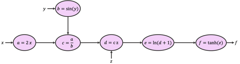
, , から始めて矢印と式に従うと、グラフは関数 と同じ値を返します。これは中間変数 を計算することで実現されます。これを順伝播と呼びます。
次に、 から始めて矢印の逆方向に進みながら各式の勾配を計算します。これを逆伝播と呼び、誤差逆伝播法の名前の由来です。
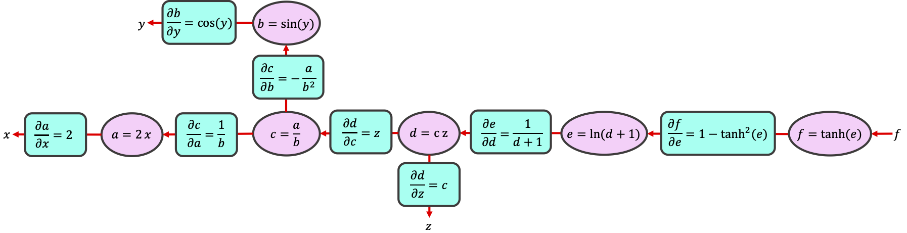
計算を中間変数の単純な演算に分解することで、連鎖律を使って任意の勾配を計算できます:
便利なことに、, , の値は順伝播時に計算・保存されているため、偏微分は中間変数 の式で簡単に表せます。
演習1.3: 連鎖律(任意)
上記の関数について、計算グラフと連鎖律を使い を計算してください。
解答を見るにはここをクリック
詳細はこちら: 計算グラフ上の微分:逆伝播
# @title Submit your feedback
content_review(f"{feedback_prefix}_Chain_Rule_Analytical_Exercise")
セクション2: PyTorch AutoGrad
所要時間の目安:約30~45分
# @title Video 4: Auto-Differentiation
from ipywidgets import widgets
from IPython.display import YouTubeVideo
from IPython.display import IFrame
from IPython.display import display


class PlayVideo(IFrame):
  def __init__(self, id, source, page=1, width=400, height=300, **kwargs):
    self.id = id
    if source == 'Bilibili':
      src = f'https://player.bilibili.com/player.html?bvid={id}&page={page}'
    elif source == 'Osf':
      src = f'https://mfr.ca-1.osf.io/render?url=https://osf.io/download/{id}/?direct%26mode=render'
    super(PlayVideo, self).__init__(src, width, height, **kwargs)


def display_videos(video_ids, W=400, H=300, fs=1):
  tab_contents = []
  for i, video_id in enumerate(video_ids):
    out = widgets.Output()
    with out:
      if video_ids[i][0] == 'Youtube':
        video = YouTubeVideo(id=video_ids[i][1], width=W,
                             height=H, fs=fs, rel=0)
        print(f'Video available at https://youtube.com/watch?v={video.id}')
      else:
        video = PlayVideo(id=video_ids[i][1], source=video_ids[i][0], width=W,
                          height=H, fs=fs, autoplay=False)
        if video_ids[i][0] == 'Bilibili':
          print(f'Video available at https://www.bilibili.com/video/{video.id}')
        elif video_ids[i][0] == 'Osf':
          print(f'Video available at https://osf.io/{video.id}')
      display(video)
    tab_contents.append(out)
  return tab_contents


video_ids = [('Youtube', 'IBYFCNyBcF8'), ('Bilibili', 'BV1UP4y1s7gv')]
tab_contents = display_videos(video_ids, W=854, H=480)
tabs = widgets.Tab()
tabs.children = tab_contents
for i in range(len(tab_contents)):
  tabs.set_title(i, video_ids[i][0])
display(tabs)
# @title Submit your feedback
content_review(f"{feedback_prefix}_AutoDifferentiation_Video")PyTorch、JAX、TensorFlowなどのディープラーニングフレームワークには、自動微分として知られる非常に効率的で高度なアルゴリズム群が備わっています。AutoGradはPyTorchの自動微分エンジンです。ここではAutoGradの基本を扱い、今後さらに学びます。
セクション2.1: 順伝播
すべては順伝播(フォワードパス)から始まります。PyTorchは変数や演算を宣言するときにすべての操作を追跡し、.backward() を呼ぶとグラフを構築します。PyTorchはイテレーションや変更のたびにグラフを再構築します(動的グラフを使用)。
勾配降下法では、学習したい変数に関する損失関数の勾配だけが必要です。これらの変数はPyTorchでは「学習可能/訓練可能パラメータ」または単に「パラメータ」と呼ばれます。ニューラルネットでは重みやバイアスが学習可能パラメータです。
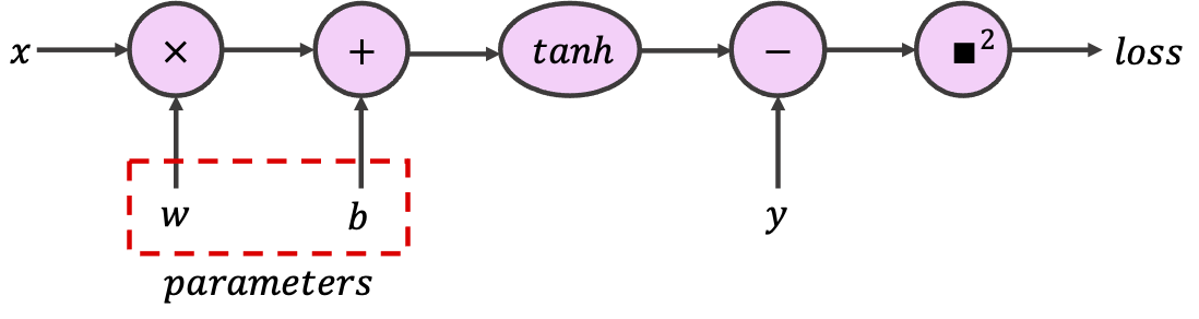
コーディング演習2.1: 計算グラフの構築
PyTorchでは、あるテンソルが学習可能パラメータを含むことを示すために、オプション引数 requires_grad を True に設定できます。PyTorchはこのテンソルを使ったすべての演算を追跡し、計算グラフを構築します。この演習では、与えられたテンソルを使って、スカラー入力と出力を持つ単一ニューロンを実装する以下のグラフを構築してください。
class SimpleGraph:
  """
  Implementing Simple Computational Graph
  """

  def __init__(self, w, b):
    """
    Initializing the SimpleGraph

    Args:
      w: float
        Initial value for weight
      b: float
        Initial value for bias

    Returns:
      Nothing
    """
    assert isinstance(w, float)
    assert isinstance(b, float)
    self.w = torch.tensor([w], requires_grad=True)
    self.b = torch.tensor([b], requires_grad=True)

  def forward(self, x):
    """
    Forward pass

    Args:
      x: torch.Tensor
        1D tensor of features

    Returns:
      prediction: torch.Tensor
        Model predictions
    """
    assert isinstance(x, torch.Tensor)
    #################################################
    ## Implement the the forward pass to calculate prediction
    ## Note that prediction is not the loss, but the value after `tanh`
    # Complete the function and remove or comment the line below
    raise NotImplementedError("Forward Pass `forward`")
    #################################################
    prediction = ...
    return prediction


def sq_loss(y_true, y_prediction):
  """
  L2 loss function

  Args:
    y_true: torch.Tensor
      1D tensor of target labels
    y_prediction: torch.Tensor
      1D tensor of predictions

  Returns:
    loss: torch.Tensor
      L2-loss (squared error)
  """
  assert isinstance(y_true, torch.Tensor)
  assert isinstance(y_prediction, torch.Tensor)
  #################################################
  ## Implement the L2-loss (squred error) given true label and prediction
  # Complete the function and remove or comment the line below
  raise NotImplementedError("Loss function `sq_loss`")
  #################################################
  loss = ...
  return loss


feature = torch.tensor([1])  # Input tensor
target = torch.tensor([7])  # Target tensor
## Uncomment to run
# simple_graph = SimpleGraph(-0.5, 0.5)
# print(f"initial weight = {simple_graph.w.item()}, "
#       f"\ninitial bias = {simple_graph.b.item()}")
# prediction = simple_graph.forward(feature)
# square_loss = sq_loss(target, prediction)
# print(f"for x={feature.item()} and y={target.item()}, "
# f"prediction={prediction.item()}, and L2 Loss = {square_loss.item()}")PyTorchがクラスや関数を自由に行き来しながら操作を追跡できることを理解することが重要です。
# @title Submit your feedback
content_review(f"{feedback_prefix}_Building_a_computational_graph_Exercise")
セクション2.2: 逆伝播
ここにすべての魔法があります。PyTorchでは、Tensor と Function が相互に結びつき、有向非巡回グラフを構築し、計算の完全な履歴を符号化します。各変数は grad_fn 属性を持ち、テンソルを作成した関数を参照します(ユーザーが作成したテンソルは grad_fn が None です)。以下の例では、テンソル c = a + b は Add 演算によって作成され、勾配関数は <AddBackward...> オブジェクトです。+ を他の単一演算(例:c = a * b や c = torch.sin(a))に置き換えて結果を確認してください。
a = torch.tensor([1.0], requires_grad=True)
b = torch.tensor([-1.0], requires_grad=True)
c = a + b
print(f'Gradient function = {c.grad_fn}')複雑な関数では、grad_fn を表示しても最後の演算のみが表示されますが、そのオブジェクトはその時点までのすべての演算を追跡しています。
print(f'Gradient function for prediction = {prediction.grad_fn}')
print(f'Gradient function for loss = {square_loss.grad_fn}')
では、逆伝播を開始するために、逆伝播を始めたいテンソルで .backward() を呼びます。通常、損失(グラフの最後のノード)で .backward() を呼びます。まず、損失の勾配を手計算しましょう:
ここで はターゲット(真のラベル)、 は予測(モデル出力)です。これをPyTorchの勾配(関連テンソルの .grad を呼ぶことで得られます)と比較できます。
重要な注意点:
-
学習可能パラメータ(
requires_gradがTrueのテンソル)は「伝染的」です。例えば、Y = W @ Xで、Xは特徴テンソル、Wは学習可能パラメータ(requires_grad)の重みテンソルの場合、生成された出力テンソルYもrequires_gradになります。したがって、Yに適用される演算はすべて計算グラフの一部になります。requires_gradのテンソルをプロットや保存したい場合は、まず.detach()メソッドでグラフから切り離す必要があります。 -
.backward()は葉ノード(対象ノードへの入力ノード)に勾配を蓄積します。損失やオプティマイザで.zero_grad()を呼ぶとすべての.grad属性をゼロにできます(詳細は autograd.backward を参照)。 -
Pythonでは変数や関連メソッドに
.method_nameでアクセスできます。 コマンドでオブジェクトの変数やメソッドを一覧できます。例:。
# Analytical gradients (Remember detaching)
ana_dloss_dw = - 2 * feature * (target - prediction.detach())*(1 - prediction.detach()**2)
ana_dloss_db = - 2 * (target - prediction.detach())*(1 - prediction.detach()**2)

square_loss.backward()  # First we should call the backward to build the graph
autograd_dloss_dw = simple_graph.w.grad  # We calculate the derivative w.r.t weights
autograd_dloss_db = simple_graph.b.grad  # We calculate the derivative w.r.t bias

print(ana_dloss_dw == autograd_dloss_dw)
print(ana_dloss_db == autograd_dloss_db)
参考文献・詳細
セクション3: PyTorchのニューラルネットモジュール (nn.Module)
所要時間の目安:約30分
# @title Video 5: PyTorch `nn` module
from ipywidgets import widgets
from IPython.display import YouTubeVideo
from IPython.display import IFrame
from IPython.display import display


class PlayVideo(IFrame):
  def __init__(self, id, source, page=1, width=400, height=300, **kwargs):
    self.id = id
    if source == 'Bilibili':
      src = f'https://player.bilibili.com/player.html?bvid={id}&page={page}'
    elif source == 'Osf':
      src = f'https://mfr.ca-1.osf.io/render?url=https://osf.io/download/{id}/?direct%26mode=render'
    super(PlayVideo, self).__init__(src, width, height, **kwargs)


def display_videos(video_ids, W=400, H=300, fs=1):
  tab_contents = []
  for i, video_id in enumerate(video_ids):
    out = widgets.Output()
    with out:
      if video_ids[i][0] == 'Youtube':
        video = YouTubeVideo(id=video_ids[i][1], width=W,
                             height=H, fs=fs, rel=0)
        print(f'Video available at https://youtube.com/watch?v={video.id}')
      else:
        video = PlayVideo(id=video_ids[i][1], source=video_ids[i][0], width=W,
                          height=H, fs=fs, autoplay=False)
        if video_ids[i][0] == 'Bilibili':
          print(f'Video available at https://www.bilibili.com/video/{video.id}')
        elif video_ids[i][0] == 'Osf':
          print(f'Video available at https://osf.io/{video.id}')
      display(video)
    tab_contents.append(out)
  return tab_contents


video_ids = [('Youtube', 'jzTbQACq7KE'), ('Bilibili', 'BV1MU4y1H7WH')]
tab_contents = display_videos(video_ids, W=854, H=480)
tabs = widgets.Tab()
tabs.children = tab_contents
for i in range(len(tab_contents)):
  tabs.set_title(i, video_ids[i][0])
display(tabs)
# @title Submit your feedback
content_review(f"{feedback_prefix}_Pytorch_nn_module_Video")PyTorchは、層(線形層、再帰層など)、様々な活性化関数や損失関数など、すぐに使えるニューラルネット構築ブロックを torch.nn モジュールにまとめています。torch.nn の層を使ってニューラルネットを構築すると、重みやバイアスはすでに requires_grad モードになっており、モデルパラメータとして登録されます。
トレーニングには3つの要素が必要です:
-
モデルパラメータ: モデルのすべての学習可能パラメータで、モデルの
.parameters()を呼ぶとアクセスできます。すべてのrequires_gradテンソルがモデルパラメータとして見なされるわけではありません。カスタムのモデルパラメータを作成するにはnn.Parameterを使います(モジュールパラメータとみなされるテンソルの一種)。 -
損失関数: 最適化対象の損失で、多くの場合正則化項と組み合わせます(数日後に登場)。
-
オプティマイザ: PyTorchは多くの最適化手法(勾配降下法の様々なバージョン)を提供します。オプティマイザはモデルの現在の状態を保持し、
step()メソッドを呼ぶと計算された勾配に基づいてパラメータを更新します。
コースの後半で、適切なモデルアーキテクチャ、損失関数、オプティマイザの選び方を詳しく学びます。
セクション3.1: PyTorchでのトレーニングループ
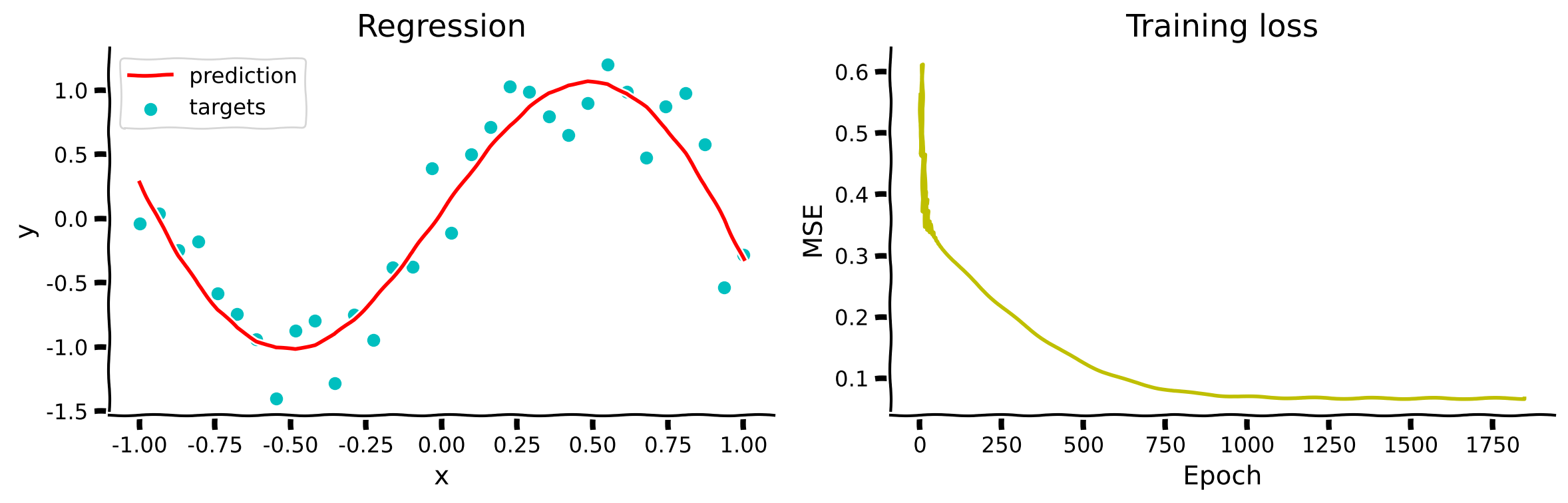
回帰問題を使ってPyTorchのトレーニングループを学びます。
課題は、単純な 回帰タスクのために、広い非線形( 活性化関数使用)ニューラルネットを訓練することです。広いニューラルネットは一般化性能が高いと考えられています。
# @markdown #### Generate the sample dataset
set_seed(seed=SEED)
n_samples = 32
inputs = torch.linspace(-1.0, 1.0, n_samples).reshape(n_samples, 1)
noise = torch.randn(n_samples, 1) / 4
targets = torch.sin(pi * inputs) + noise
plt.figure(figsize=(8, 5))
plt.scatter(inputs, targets, c='c')
plt.xlabel('x (inputs)')
plt.ylabel('y (targets)')
plt.show()
512ニューロンの非常に広い1層隠れ層のニューラルネットを nn.Tanh() 活性化関数で定義しましょう。
class WideNet(nn.Module):
  """
   A Wide neural network with a single hidden layer
   Structure is as follows:
   nn.Sequential(
        nn.Linear(1, n_cells) + nn.Tanh(), # Fully connected layer with tanh activation
        nn.Linear(n_cells, 1) # Final fully connected layer
    )
  """

  def __init__(self):
    """
    Initializing the parameters of WideNet

    Args:
      None

    Returns:
      Nothing
    """
    n_cells = 512
    super().__init__()
    self.layers = nn.Sequential(
        nn.Linear(1, n_cells),
        nn.Tanh(),
        nn.Linear(n_cells, 1),
    )

  def forward(self, x):
    """
    Forward pass of WideNet

    Args:
      x: torch.Tensor
        2D tensor of features

    Returns:
      Torch tensor of model predictions
    """
    return self.layers(x)
ニューラルネットのインスタンスを作成し、そのパラメータを表示します。
# Creating an instance
set_seed(seed=SEED)
wide_net = WideNet()
print(wide_net)
# Create a mse loss function
loss_function = nn.MSELoss()
# Stochstic Gradient Descent optimizer (you will learn about momentum soon)
lr = 0.003 # Learning rate
sgd_optimizer = torch.optim.SGD(wide_net.parameters(), lr=lr, momentum=0.9)PyTorchのトレーニングはインタラクティブで、好きなだけ訓練イテレーションを実行し、各イテレーション後に結果を確認できます。
1回のトレーニングイテレーションを実行しましょう。セルを複数回実行してパラメータが更新され、損失が減少する様子を確認できます。このコードブロックは今後のすべての基礎です。すべてのコマンドを行ごとに理解し、ポッド内で目的を議論してください。
# Reset all gradients to zero
sgd_optimizer.zero_grad()

# Forward pass (Compute the output of the model on the features (inputs))
prediction = wide_net(inputs)

# Compute the loss
loss = loss_function(prediction, targets)
print(f'Loss: {loss.item()}')

# Perform backpropagation to build the graph and compute the gradients
loss.backward()

# Optimizer takes a tiny step in the steepest direction (negative of gradient)
# and "updates" the weights and biases of the network
sgd_optimizer.step()
コーディング演習3.1: トレーニングループ
これまで学んだことを使って、以下の train 関数を完成させてください。
def train(features, labels, model, loss_fun, optimizer, n_epochs):
  """
  Training function

  Args:
    features: torch.Tensor
      Features (input) with shape torch.Size([n_samples, 1])
    labels: torch.Tensor
      Labels (targets) with shape torch.Size([n_samples, 1])
    model: torch nn.Module
      The neural network
    loss_fun: function
      Loss function
    optimizer: function
      Optimizer
    n_epochs: int
      Number of training iterations

  Returns:
    loss_record: list
      Record (evolution) of training losses
  """
  loss_record = []  # Keeping recods of loss

  for i in range(n_epochs):
    #################################################
    ## Implement the missing parts of the training loop
    # Complete the function and remove or comment the line below
    raise NotImplementedError("Training loop `train`")
    #################################################
    ...  # Set gradients to 0
    predictions = ...  # Compute model prediction (output)
    loss = ...  # Compute the loss
    ...  # Compute gradients (backward pass)
    ...  # Update parameters (optimizer takes a step)

    loss_record.append(loss.item())
  return loss_record


set_seed(seed=2021)
epochs = 1847 # Cauchy, Exercices d'analyse et de physique mathematique (1847)
## Uncomment to run
# losses = train(inputs, targets, wide_net, loss_function, sgd_optimizer, epochs)
# ex3_plot(wide_net, inputs, targets, epochs, losses)出力例:
# @title Submit your feedback
content_review(f"{feedback_prefix}_Training_loop_Exercise")
まとめ
本チュートリアルでは、ディープラーニングの最も基本的な概念の一つである計算グラフと、勾配降下法および誤差逆伝播アルゴリズムによるネットワークの学習方法を扱いました。PyTorchモジュールを使ってこれらを確認し、解析的解とPyTorchが直接提供する解を比較しました。
# @title Video 6: Tutorial 1 Wrap-up
from ipywidgets import widgets
from IPython.display import YouTubeVideo
from IPython.display import IFrame
from IPython.display import display


class PlayVideo(IFrame):
  def __init__(self, id, source, page=1, width=400, height=300, **kwargs):
    self.id = id
    if source == 'Bilibili':
      src = f'https://player.bilibili.com/player.html?bvid={id}&page={page}'
    elif source == 'Osf':
      src = f'https://mfr.ca-1.osf.io/render?url=https://osf.io/download/{id}/?direct%26mode=render'
    super(PlayVideo, self).__init__(src, width, height, **kwargs)


def display_videos(video_ids, W=400, H=300, fs=1):
  tab_contents = []
  for i, video_id in enumerate(video_ids):
    out = widgets.Output()
    with out:
      if video_ids[i][0] == 'Youtube':
        video = YouTubeVideo(id=video_ids[i][1], width=W,
                             height=H, fs=fs, rel=0)
        print(f'Video available at https://youtube.com/watch?v={video.id}')
      else:
        video = PlayVideo(id=video_ids[i][1], source=video_ids[i][0], width=W,
                          height=H, fs=fs, autoplay=False)
        if video_ids[i][0] == 'Bilibili':
          print(f'Video available at https://www.bilibili.com/video/{video.id}')
        elif video_ids[i][0] == 'Osf':
          print(f'Video available at https://osf.io/{video.id}')
      display(video)
    tab_contents.append(out)
  return tab_contents


video_ids = [('Youtube', 'TvZURbcnXc4'), ('Bilibili', 'BV1Pg41177VU')]
tab_contents = display_videos(video_ids, W=854, H=480)
tabs = widgets.Tab()
tabs.children = tab_contents
for i in range(len(tab_contents)):
  tabs.set_title(i, video_ids[i][0])
display(tabs)
# @title Submit your feedback
content_review(f"{feedback_prefix}_Tutorial_1_WrapUp_Video")