チュートリアル 4: 器具変数（Instrumental Variables）

第3週5日目: ネットワーク因果性

Neuromatch Academyによる

コンテンツ作成者: Ari Benjamin, Tony Liu, Konrad Kording

コンテンツレビュアー: Mike X Cohen, Madineh Sarvestani, Yoni Friedman, Ella Batty, Michael Waskom

制作編集者: Gagana B, Spiros Chavlis

チュートリアルの目的

推定所要時間: 1時間5分

本日は因果性を検証する日の最終チュートリアルです。以下は本日扱った内容の大まかな概要であり、このノートブックで重点的に扱うセクションは太字で示しています:

因果性の定義をマスターする
因果性の推定が可能であることを理解する
4つの異なる手法を学び、それらが失敗する状況を理解する

介入（perturbations）
相関（correlations）
同時フィッティング／回帰（simultaneous fitting/regression）
器具変数（instrumental variables）

チュートリアル4の目的

チュートリアル3では、同時フィッティングのようなより高度な手法でも、除外変数バイアスがあると因果性を捉えられないことを見ました。では、システムを介入できない場合に有効な因果推定を得るためにはどんな手法があるのでしょうか？ここでは:

実験データを必要としない因果分析の手法である器具変数について学ぶ
器具変数分析の利点と制限を探る
- 回帰で見られる除外変数バイアスに対処する
- 他の手法に比べてサンプルサイズ効率は劣る
- 因果効果を特定するためにシステムに特定の形のランダム性が必要となる

# @title Tutorial slides
# @markdown These are the slides for the videos in all tutorials today
from IPython.display import IFrame
link_id = "gp4m9"
print(f"If you want to download the slides: https://osf.io/download/{link_id}/")
IFrame(src=f"https://mfr.ca-1.osf.io/render?url=https://osf.io/{link_id}/?direct%26mode=render%26action=download%26mode=render", width=854, height=480)

セットアップ

# @title Install and import feedback gadget


from vibecheck import DatatopsContentReviewContainer
def content_review(notebook_section: str):
    return DatatopsContentReviewContainer(
        "",  # No text prompt
        notebook_section,
        {
            "url": "https://pmyvdlilci.execute-api.us-east-1.amazonaws.com/klab",
            "name": "neuromatch_cn",
            "user_key": "y1x3mpx5",
        },
    ).render()


feedback_prefix = "W3D5_T4"

# Imports
import numpy as np
import matplotlib.pyplot as plt
from mpl_toolkits.axes_grid1 import make_axes_locatable

from sklearn.multioutput import MultiOutputRegressor
from sklearn.linear_model import LinearRegression, Lasso

# @title Figure Settings
import logging
logging.getLogger('matplotlib.font_manager').disabled = True

import ipywidgets as widgets  # interactive display
%config InlineBackend.figure_format = 'retina'
plt.style.use("https://raw.githubusercontent.com/NeuromatchAcademy/course-content/main/nma.mplstyle")

# @title Plotting Functions

def see_neurons(A, ax, show=False):
  """
  Visualizes the connectivity matrix.

  Args:
      A (np.ndarray): the connectivity matrix of shape (n_neurons, n_neurons)
      ax (plt.axis): the matplotlib axis to display on

  Returns:
      Nothing, but visualizes A.
  """
  A = A.T  # make up for opposite connectivity
  n = len(A)
  ax.set_aspect('equal')
  thetas = np.linspace(0, np.pi * 2, n,endpoint=False)
  x, y = np.cos(thetas), np.sin(thetas),
  ax.scatter(x, y, c='k',s=150)
  A = A / A.max()
  for i in range(n):
    for j in range(n):
      if A[i, j] > 0:
        ax.arrow(x[i], y[i], x[j] - x[i], y[j] - y[i], color='k', alpha=A[i, j], head_width=.15,
                width = A[i,j] / 25, shape='right', length_includes_head=True)
  ax.axis('off')
  if show:
    plt.show()


def plot_neural_activity(X):
  """Plot first 10 timesteps of neural activity

  Args:
    X (ndarray): neural activity (n_neurons by timesteps)
  """
  f, ax = plt.subplots()
  im = ax.imshow(X[:, :10], aspect='auto')
  divider = make_axes_locatable(ax)
  cax1 = divider.append_axes("right", size="5%", pad=0.15)
  plt.colorbar(im, cax=cax1)
  ax.set(xlabel='Timestep', ylabel='Neuron', title='Simulated Neural Activity')
  plt.show()


def compare_granger_connectivity(A, reject_null, selected_neuron):
  """Plot granger connectivity vs true

  Args:
    A (ndarray): true connectivity (n_neurons by n_neurons)
    reject_null (list): outcome of granger causality, length n_neurons
    selecte_neuron (int): the neuron we are plotting connectivity from

  """
  fig, axs = plt.subplots(1, 2, figsize=(10, 5))

  im = axs[0].imshow(A[:, [selected_neuron]], cmap='coolwarm', aspect='auto')
  plt.colorbar(im, ax=axs[0])
  axs[0].set_xticks([0])
  axs[0].set_xticklabels([f"Neuron {selected_neuron}"])
  axs[0].set_title(f"True connectivity")

  im = axs[1].imshow(np.array([reject_null]).transpose(),
                     cmap='coolwarm', aspect='auto')
  plt.colorbar(im, ax=axs[1])
  axs[1].set_xticks([0])
  axs[1].set_xticklabels([f"Neuron {selected_neuron}"])
  axs[1].set_title(f"Granger causality connectivity")
  plt.show()


def plot_performance_vs_eta(etas, corr_data):
  """ Plot IV estimation performance as a function of instrument strength

    Args:
      etas (list): list of instrument strengths
      corr_data (ndarray): n_trials x len(etas) array where each element is the correlation
        between true and estimated connectivity matries for that trial and
        instrument strength

  """
  corr_mean = corr_data.mean(axis=0)
  corr_std = corr_data.std(axis=0)

  plt.plot(etas, corr_mean)
  plt.fill_between(etas, corr_mean - corr_std, corr_mean + corr_std, alpha=.2)
  plt.xlim([etas[0], etas[-1]])
  plt.title("IV performance as a function of instrument strength")
  plt.ylabel("Correlation b.t. IV and true connectivity")
  plt.xlabel("Strength of instrument (eta)")
  plt.show()

# @title Helper Functions

def sigmoid(x):
    """
    Compute sigmoid nonlinearity element-wise on x.

    Args:
        x (np.ndarray): the numpy data array we want to transform
    Returns
        (np.ndarray): x with sigmoid nonlinearity applied
    """
    return 1 / (1 + np.exp(-x))


def logit(x):
    """

    Applies the logit (inverse sigmoid) transformation

    Args:
        x (np.ndarray): the numpy data array we want to transform
    Returns
        (np.ndarray): x with logit nonlinearity applied
    """
    return np.log(x/(1-x))


def create_connectivity(n_neurons, random_state=42, p=0.9):
    """
    Generate our nxn causal connectivity matrix.

    Args:
        n_neurons (int): the number of neurons in our system.
        random_state (int): random seed for reproducibility

    Returns:
        A (np.ndarray): our 0.1 sparse connectivity matrix
    """
    np.random.seed(random_state)
    A_0 = np.random.choice([0, 1], size=(n_neurons, n_neurons), p=[p, 1 - p])

    # set the timescale of the dynamical system to about 100 steps
    _, s_vals, _ = np.linalg.svd(A_0)
    A = A_0 / (1.01 * s_vals[0])

    # _, s_val_test, _ = np.linalg.svd(A)
    # assert s_val_test[0] < 1, "largest singular value >= 1"

    return A


def simulate_neurons(A, timesteps, random_state=42):
    """
    Simulates a dynamical system for the specified number of neurons and timesteps.

    Args:
        A (np.array): the connectivity matrix
        timesteps (int): the number of timesteps to simulate our system.
        random_state (int): random seed for reproducibility

    Returns:
        - X has shape (n_neurons, timeteps).
    """
    np.random.seed(random_state)

    n_neurons = len(A)
    X = np.zeros((n_neurons, timesteps))

    for t in range(timesteps - 1):
        # solution
        epsilon = np.random.multivariate_normal(np.zeros(n_neurons), np.eye(n_neurons))
        X[:, t + 1] = sigmoid(A.dot(X[:, t]) + epsilon)

        assert epsilon.shape == (n_neurons,)
    return X


def get_sys_corr(n_neurons, timesteps, random_state=42, neuron_idx=None):
    """
    A wrapper function for our correlation calculations between A and R.

    Args:
        n_neurons (int): the number of neurons in our system.
        timesteps (int): the number of timesteps to simulate our system.
        random_state (int): seed for reproducibility
        neuron_idx (int): optionally provide a neuron idx to slice out

    Returns:
        A single float correlation value representing the similarity between A and R
    """

    A = create_connectivity(n_neurons, random_state)
    X = simulate_neurons(A, timesteps)

    R = correlation_for_all_neurons(X)

    return np.corrcoef(A.flatten(), R.flatten())[0, 1]


def correlation_for_all_neurons(X):
  """Computes the connectivity matrix for the all neurons using correlations

    Args:
        X: the matrix of activities

    Returns:
        estimated_connectivity (np.ndarray): estimated connectivity for the selected neuron, of shape (n_neurons,)
  """
  n_neurons = len(X)
  S = np.concatenate([X[:, 1:], X[:, :-1]], axis=0)
  R = np.corrcoef(S)[:n_neurons, n_neurons:]
  return R


def print_corr(v1, v2, corrs, idx_dict):
    """Helper function for formatting print statements for correlations"""
    text_dict = {'Z':'taxes', 'T':'# cigarettes', 'C':'SES status', 'Y':'birth weight'}
    print("Correlation between {} and {} ({} and {}): {:.3f}".format(v1, v2, text_dict[v1], text_dict[v2], corrs[idx_dict[v1], idx_dict[v2]]))


def get_regression_estimate(X, neuron_idx=None):
    """
    Estimates the connectivity matrix using lasso regression.

    Args:
        X (np.ndarray): our simulated system of shape (n_neurons, timesteps)
        neuron_idx (int): optionally provide a neuron idx to compute connectivity for
    Returns:
        V (np.ndarray): estimated connectivity matrix of shape (n_neurons, n_neurons).
                        if neuron_idx is specified, V is of shape (n_neurons,).
    """
    n_neurons = X.shape[0]

    # Extract Y and W as defined above
    W = X[:, :-1].transpose()
    if neuron_idx is None:
        Y = X[:, 1:].transpose()
    else:
        Y = X[[neuron_idx], 1:].transpose()

    # apply inverse sigmoid transformation
    Y = logit(Y)

    # fit multioutput regression
    regression = MultiOutputRegressor(Lasso(fit_intercept=False, alpha=0.01), n_jobs=-1)

    regression.fit(W,Y)

    if neuron_idx is None:
        V = np.zeros((n_neurons, n_neurons))
        for i, estimator in enumerate(regression.estimators_):
            V[i, :] = estimator.coef_
    else:
        V = regression.estimators_[0].coef_

    return V


def get_regression_corr(n_neurons, timesteps, random_state, observed_ratio, regression_args, neuron_idx=None):
    """
    A wrapper function for our correlation calculations between A and the V estimated
    from regression.

    Args:
        n_neurons (int): the number of neurons in our system.
        timesteps (int): the number of timesteps to simulate our system.
        random_state (int): seed for reproducibility
        observed_ratio (float): the proportion of n_neurons observed, must be between 0 and 1.
        regression_args (dict): dictionary of lasso regression arguments and hyperparameters
        neuron_idx (int): optionally provide a neuron idx to compute connectivity for

    Returns:
        A single float correlation value representing the similarity between A and R
    """
    assert (observed_ratio > 0) and (observed_ratio <= 1)

    A = create_connectivity(n_neurons, random_state)
    X = simulate_neurons(A, timesteps)

    sel_idx = np.clip(int(n_neurons*observed_ratio), 1, n_neurons)

    sel_X = X[:sel_idx, :]
    sel_A = A[:sel_idx, :sel_idx]

    sel_V = get_regression_estimate(sel_X, neuron_idx=neuron_idx)
    if neuron_idx is None:
        return np.corrcoef(sel_A.flatten(), sel_V.flatten())[1, 0]
    else:
        return np.corrcoef(sel_A[neuron_idx, :], sel_V)[1, 0]


def get_regression_estimate_full_connectivity(X):
    """
    Estimates the connectivity matrix using lasso regression.

    Args:
        X (np.ndarray): our simulated system of shape (n_neurons, timesteps)
        neuron_idx (int): optionally provide a neuron idx to compute connectivity for
    Returns:
        V (np.ndarray): estimated connectivity matrix of shape (n_neurons, n_neurons).
                        if neuron_idx is specified, V is of shape (n_neurons,).
    """
    n_neurons = X.shape[0]

    # Extract Y and W as defined above
    W = X[:, :-1].transpose()
    Y = X[:, 1:].transpose()

    # apply inverse sigmoid transformation
    Y = logit(Y)

    # fit multioutput regression
    reg = MultiOutputRegressor(Lasso(fit_intercept=False, alpha=0.01, max_iter=200), n_jobs=-1)
    reg.fit(W, Y)

    V = np.zeros((n_neurons, n_neurons))
    for i, estimator in enumerate(reg.estimators_):
        V[i, :] = estimator.coef_

    return V


def get_regression_corr_full_connectivity(n_neurons, A, X, observed_ratio, regression_args):
    """
    A wrapper function for our correlation calculations between A and the V estimated
    from regression.

    Args:
        n_neurons (int): number of neurons
        A (np.ndarray): connectivity matrix
        X (np.ndarray): dynamical system
        observed_ratio (float): the proportion of n_neurons observed, must be between 0 and 1.
        regression_args (dict): dictionary of lasso regression arguments and hyperparameters

    Returns:
        A single float correlation value representing the similarity between A and R
    """
    assert (observed_ratio > 0) and (observed_ratio <= 1)

    sel_idx = np.clip(int(n_neurons*observed_ratio), 1, n_neurons)

    sel_X = X[:sel_idx, :]
    sel_A = A[:sel_idx, :sel_idx]

    sel_V = get_regression_estimate_full_connectivity(sel_X)
    return np.corrcoef(sel_A.flatten(), sel_V.flatten())[1,0], sel_V

上で定義したヘルパー関数は以下の通りです:

sigmoid: チュートリアル1で紹介した、入力に対して要素ごとにシグモイド非線形変換を行う関数
logit: チュートリアル3で紹介した、ロジット（シグモイドの逆変換）を適用する関数
create_connectivity: チュートリアル1で紹介した、nxnの因果的結合行列を生成する関数
simulate_neurons: チュートリアル1で紹介した、指定したニューロン数とタイムステップ数で動的システムをシミュレートする関数
get_sys_corr: チュートリアル2で紹介した、AとR間の相関計算のラッパー関数
correlation_for_all_neurons: チュートリアル2で紹介した、全ニューロンの結合行列を相関から計算する関数
print_corr: 相関の表示を整形する関数
get_regression_estimate: チュートリアル3で紹介した、ラッソ回帰を用いて結合行列を推定する関数
get_regression_corr: 回帰で推定したVとAの相関計算のラッパー関数
get_regression_estimate_full_connectivity: チュートリアル3で紹介した、ラッソ回帰で結合行列全体を推定する関数
get_regression_corr_full_connectivity: チュートリアル3で紹介した、回帰で推定したVとAの相関計算のラッパー関数

セクション1: 器具変数（Instrumental Variables）

# @title Video 1: Instrumental Variables
from ipywidgets import widgets
from IPython.display import YouTubeVideo
from IPython.display import IFrame
from IPython.display import display


class PlayVideo(IFrame):
  def __init__(self, id, source, page=1, width=400, height=300, **kwargs):
    self.id = id
    if source == 'Bilibili':
      src = f'https://player.bilibili.com/player.html?bvid={id}&page={page}'
    elif source == 'Osf':
      src = f'https://mfr.ca-1.osf.io/render?url=https://osf.io/download/{id}/?direct%26mode=render'
    super(PlayVideo, self).__init__(src, width, height, **kwargs)


def display_videos(video_ids, W=400, H=300, fs=1):
  tab_contents = []
  for i, video_id in enumerate(video_ids):
    out = widgets.Output()
    with out:
      if video_ids[i][0] == 'Youtube':
        video = YouTubeVideo(id=video_ids[i][1], width=W,
                             height=H, fs=fs, rel=0)
        print(f'Video available at https://youtube.com/watch?v={video.id}')
      else:
        video = PlayVideo(id=video_ids[i][1], source=video_ids[i][0], width=W,
                          height=H, fs=fs, autoplay=False)
        if video_ids[i][0] == 'Bilibili':
          print(f'Video available at https://www.bilibili.com/video/{video.id}')
        elif video_ids[i][0] == 'Osf':
          print(f'Video available at https://osf.io/{video.id}')
      display(video)
    tab_contents.append(out)
  return tab_contents


video_ids = [('Youtube', '0gkav6BS4-w'), ('Bilibili', 'BV1of4y1R7L1')]
tab_contents = display_videos(video_ids, W=854, H=480)
tabs = widgets.Tab()
tabs.children = tab_contents
for i in range(len(tab_contents)):
  tabs.set_title(i, video_ids[i][0])
display(tabs)

# @title Submit your feedback
content_review(f"{feedback_prefix}_Instrumental_Variables_Video")

システム内に観測可能な自然発生的なランダム性がある場合、これが因果効果を回復するために使える介入の代わりになります。これを器具変数と呼びます。大まかに言うと、器具変数は以下の条件を満たす必要があります:

観測可能であること
関心のある共変量に影響を与えること
その共変量を通じてのみ結果に影響を与え、それ以外には影響を与えないこと

このような条件を満たすものを自然界で見つけるのは稀ですが、見つかれば非常に強力です。

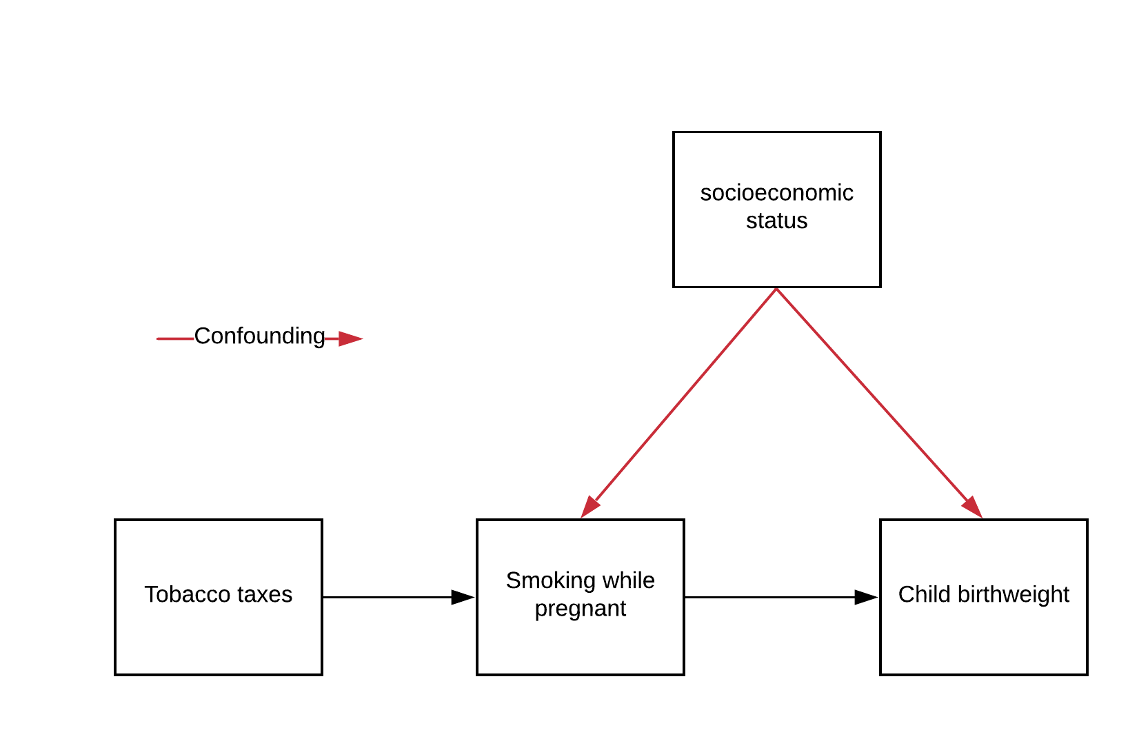
セクション1.1: 器具変数の非神経科学的な例

古典的な例は、妊娠中の喫煙が乳児の出生体重に与える影響を推定することです。負の相関はありますが、それは因果的でしょうか？残念ながら多くの交絡因子が出生体重と喫煙の両方に影響を与えています。富裕度が大きな要因です。

すべてをコントロールする代わりに、器具変数を見つけることができます。ここでの器具変数は州のたばこ税です。これらは

観測可能である
たばこ消費に影響を与える
たばこを通じてのみ出生体重に影響を与え、それ以外には影響を与えない

器具変数の力を使うことで、すべてを厳密にコントロールしなくても因果効果を推定できます。

上記のたばこ例を以下の記法で表現しましょう:

$Z_{\text{taxes}}$ : たばこ税の器具変数。システム内で妊娠中の喫煙傾向にのみ影響を与える
$T_{\text{smoking}}$ : 妊娠中に1日に吸うたばこの本数。ランダム化試験でいう「処置」
$C_{\text{SES}}$ : 社会経済的地位（高いほど裕福）、観測されなければ交絡因子
$Y_{\text{birthweight}}$ : 乳児の出生体重（グラム）、関心のある結果変数

システムの関数は以下のように仮定します:

$Y_{\text{birthweight}} = 3000 + C_{\text{SES}} - 2T_{\text{smoking}},$

さらに、 $C_{\text{SES}}$ と $T_{\text{smoking}}$ は負の相関があるとします。

推定したい因果効果は $T_{\text{smoking}}$ の係数 $-2$ で、妊娠中に1本多くたばこを吸うと出生体重が2グラム減ることを意味します。

以下のコードセルでは、この構造を持つ共分散行列を用意しているので、変数間の相関を確認してください。

# @markdown Execute this cell to see correlations with C
# run this code below to generate our setup
idx_dict = {
    'Z': 0,
    'T': 1,
    'C': 2,
    'Y': 3
}
# vars:             Z    T    C
covar = np.array([[1.0, 0.5, 0.0],  # Z
                  [0.5, 1.0, -0.5],  # T
                  [0.0, -0.5, 1.0]])  # C
# vars:  Z  T  C
means = [0, 5, 2]

# generate some data
np.random.seed(42)
data = np.random.multivariate_normal(mean=means, cov=2 * covar, size=2000)

# generate Y from our equation above
Y = 3000 + data[:, idx_dict['C']] - (2 * (data[:, idx_dict['T']]))

data = np.concatenate([data, Y.reshape(-1, 1)], axis=1)

Z = data[:, [idx_dict['Z']]]
T = data[:, [idx_dict['T']]]
C = data[:, [idx_dict['C']]]
Y = data[:, [idx_dict['Y']]]

corrs = np.corrcoef(data.transpose())

print_corr('C', 'T', corrs, idx_dict)
print_corr('C', 'Y', corrs, idx_dict)

グラフで示した通り、 $C_{\text{SES}}$ は $T_{\text{smoking}}$ と $Y_{\text{birthweight}}$ の両方と相関があり、 $C_{\text{SES}}$ が分析に含まれなければ交絡因子となります。 $C_{\text{SES}}$ は観測・定量化が難しいと仮定し、回帰に利用できないとします。これは前回のチュートリアルで見た除外変数バイアスの例です。

では、 $Z_{\text{taxes}}$ は器具変数の条件1, 2, 3を満たしているでしょうか？

#@markdown Execute this cell to see correlations of Z
print("Condition 2?")
print_corr('Z', 'T', corrs, idx_dict)
print("Condition 3?")
print_corr('Z', 'C', corrs, idx_dict)

完璧です！ $Z_{\text{taxes}}$ は $T_{\text{smoking}}$ と相関があり（#2）、 $C_{\text{SES}}$ とは無相関（#3）です。さらに $Z_{\text{taxes}}$ は観測可能（#1）なので、器具変数の3つの条件を満たしています:

$Z_{\text{taxes}}$ は観測可能
$Z_{\text{taxes}}$ は $T_{\text{smoking}}$ に影響を与える
$Z_{\text{taxes}}$ は $T_{\text{smoking}}$ を通じてのみ $Y_{\text{birthweight}}$ に影響を与え（すなわち $Z_{\text{taxes}}$ は $C_{\text{SES}}$ に影響を与えず、影響も受けない）

セクション1.2: 器具変数の仕組み（概要）

器具変数をイメージしやすくするには、器具変数は「処置に影響を与える観測可能な『ランダム性の源』」と考えるとよいでしょう。これはチュートリアル1で扱った介入に似ています。

では実際に器具変数をどう使うのでしょうか？ポイントは、処置のうち器具変数の影響だけによる成分を抽出することです。この成分を $\hat{T}$ と呼びます。

\hat{T}\leftarrow \text{交絡されていない}Tの成分

$\hat{T}$ の取得は簡単で、器具変数 $Z$ のみを説明変数とした回帰の予測値です。

この交絡されていない成分を得たら、結果を $\hat{T}$ に回帰するだけで因果効果を推定できます。

セクション1.3: 2段階最小二乗法によるIV推定

器具変数推定の基本手法は**2段階最小二乗法（two-stage least squares）**です。

2つの回帰を行います:

第1段階では、 $T_{\text{smoking}}$ を $Z_{\text{taxes}}$ で回帰し、パラメータ $\hat{\alpha}$ を推定して $\hat{T}_{\text{smoking}}$ を得ます:

\hat{T}_{\text{smoking}} = \hat{\alpha} Z_{\text{taxes}}

第2段階では、 $Y_{\text{birthweight}}$ を $\hat{T}_{\text{smoking}}$ で回帰し、因果効果の推定値 $\hat{\beta}$ を得ます:

\hat{Y}_{\text{birthweight}} = \hat{\beta} \hat{T}_{\text{smoking}}

第1段階は、前述の通り $T_{\text{smoking}}$ の交絡されていない成分（すなわち交絡因子 $C_{\text{SES}}$ の影響を受けていない部分）を推定します。

第2段階では、この交絡されていない成分 $\hat{T}_{\text{smoking}}$ を使って、喫煙が出生体重 $\hat{Y}_{\text{birthweight}}$ に与える影響を推定します。

次の2つの演習で、この仕組みを詳しく見ていきます。

セクション 1.3.1: 最小二乗回帰ステージ1

# @title Video 2: Stage 1
from ipywidgets import widgets
from IPython.display import YouTubeVideo
from IPython.display import IFrame
from IPython.display import display


class PlayVideo(IFrame):
  def __init__(self, id, source, page=1, width=400, height=300, **kwargs):
    self.id = id
    if source == 'Bilibili':
      src = f'https://player.bilibili.com/player.html?bvid={id}&page={page}'
    elif source == 'Osf':
      src = f'https://mfr.ca-1.osf.io/render?url=https://osf.io/download/{id}/?direct%26mode=render'
    super(PlayVideo, self).__init__(src, width, height, **kwargs)


def display_videos(video_ids, W=400, H=300, fs=1):
  tab_contents = []
  for i, video_id in enumerate(video_ids):
    out = widgets.Output()
    with out:
      if video_ids[i][0] == 'Youtube':
        video = YouTubeVideo(id=video_ids[i][1], width=W,
                             height=H, fs=fs, rel=0)
        print(f'Video available at https://youtube.com/watch?v={video.id}')
      else:
        video = PlayVideo(id=video_ids[i][1], source=video_ids[i][0], width=W,
                          height=H, fs=fs, autoplay=False)
        if video_ids[i][0] == 'Bilibili':
          print(f'Video available at https://www.bilibili.com/video/{video.id}')
        elif video_ids[i][0] == 'Osf':
          print(f'Video available at https://osf.io/{video.id}')
      display(video)
    tab_contents.append(out)
  return tab_contents


video_ids = [('Youtube', '4WT0KrySRTg'), ('Bilibili', 'BV1jK4y1x7q5')]
tab_contents = display_videos(video_ids, W=854, H=480)
tabs = widgets.Tab()
tabs.children = tab_contents
for i in range(len(tab_contents)):
  tabs.set_title(i, video_ids[i][0])
display(tabs)

# @title Submit your feedback
content_review(f"{feedback_prefix}_Stage_1_Video")

コーディング演習 1.3.1: 回帰ステージ1の計算

$T_{\text{smoking}}$ を $Z_\text{taxes}$ に回帰して $\hat{T}_{\text{smoking}}$ を計算しましょう。次に、 $C_{\text{SES}}$ と $T_{\text{smoking}}$ の相関と $C_{\text{SES}}$ と $\hat{T}_{\text{smoking}}$ の相関を比較して、推定値にまだ交絡があるかどうかを確認します。

提案

すでに scikit-learn からインポートされている LinearRegression() モデルを使う
パラメータ設定は fit_intercept=True のみを使う
LinearRegression.fit() に渡すパラメータの順序を必ず確認すること

def fit_first_stage(T, Z):
  """
  Estimates T_hat as the first stage of a two-stage least squares.

  Args:
      T (np.ndarray): our observed, possibly confounded, treatment of shape (n, 1)
      Z (np.ndarray): our observed instruments of shape (n, 1)

  Returns
      T_hat (np.ndarray): our estimate of the unconfounded portion of T
  """

  ############################################################################
  ## Insert your code here to fit the first stage of the 2-stage least squares
  ## estimate.
  ## Fill out function and remove
  raise NotImplementedError('Please complete fit_first_stage function')
  ############################################################################

  # Initialize linear regression model
  stage1 = LinearRegression(...)

  # Fit linear regression model
  stage1.fit(...)

  # Predict T_hat using linear regression model
  T_hat = stage1.predict(...)

  return T_hat


# Estimate T_hat
T_hat = fit_first_stage(T, Z)

# Get correlations
T_C_corr = np.corrcoef(T.transpose(), C.transpose())[0, 1]
T_hat_C_corr = np.corrcoef(T_hat.transpose(), C.transpose())[0, 1]

# Print correlations
print(f"Correlation between T and C: {T_C_corr:.3f}")
print(f"Correlation between T_hat and C: {T_hat_C_corr:.3f}")

$T$ と $C$ の相関は -0.483、 $\hat{T}$ と $C$ の相関は 0.009 になるはずです。

解答を見る$

# @title Submit your feedback
content_review(f"{feedback_prefix}_Compute_regression_stage_1_Exercise")

セクション 1.3.2: 最小二乗回帰ステージ2

# @title Video 3: Stage 2
from ipywidgets import widgets
from IPython.display import YouTubeVideo
from IPython.display import IFrame
from IPython.display import display


class PlayVideo(IFrame):
  def __init__(self, id, source, page=1, width=400, height=300, **kwargs):
    self.id = id
    if source == 'Bilibili':
      src = f'https://player.bilibili.com/player.html?bvid={id}&page={page}'
    elif source == 'Osf':
      src = f'https://mfr.ca-1.osf.io/render?url=https://osf.io/download/{id}/?direct%26mode=render'
    super(PlayVideo, self).__init__(src, width, height, **kwargs)


def display_videos(video_ids, W=400, H=300, fs=1):
  tab_contents = []
  for i, video_id in enumerate(video_ids):
    out = widgets.Output()
    with out:
      if video_ids[i][0] == 'Youtube':
        video = YouTubeVideo(id=video_ids[i][1], width=W,
                             height=H, fs=fs, rel=0)
        print(f'Video available at https://youtube.com/watch?v={video.id}')
      else:
        video = PlayVideo(id=video_ids[i][1], source=video_ids[i][0], width=W,
                          height=H, fs=fs, autoplay=False)
        if video_ids[i][0] == 'Bilibili':
          print(f'Video available at https://www.bilibili.com/video/{video.id}')
        elif video_ids[i][0] == 'Osf':
          print(f'Video available at https://osf.io/{video.id}')
      display(video)
    tab_contents.append(out)
  return tab_contents


video_ids = [('Youtube', 'F-_m_Vgv75I'), ('Bilibili', 'BV1Kv411q7Wx')]
tab_contents = display_videos(video_ids, W=854, H=480)
tabs = widgets.Tab()
tabs.children = tab_contents
for i in range(len(tab_contents)):
  tabs.set_title(i, video_ids[i][0])
display(tabs)

# @title Submit your feedback
content_review(f"{feedback_prefix}_Stage_2_Video")

コーディング演習 1.3.2: IV推定量の計算

次に第2段階を実装しましょう！以下の $fit_second_stage()$ 関数を完成させてください。ここでも切片ありの線形回帰モデルを使います。演習1の関数（fit_first_stage）とこの関数を使って、2段階回帰モデル全体を推定します。これにより、喫煙本数 ( $T$ ) が出生体重 ( $Y$ ) に与える推定因果効果を得ます。

def fit_second_stage(T_hat, Y):
  """
  Estimates a scalar causal effect from 2-stage least squares regression using
  an instrument.

  Args:
      T_hat (np.ndarray): the output of the first stage regression
      Y (np.ndarray): our observed response (n, 1)

  Returns:
      beta (float): the estimated causal effect
  """
  ############################################################################
  ## Insert your code here to fit the second stage of the 2-stage least squares
  ## estimate.
  ## Fill out function and remove
  raise NotImplementedError('Please complete fit_second_stage function')
  ############################################################################

  # Initialize linear regression model
  stage2 = LinearRegression(...)

  # Fit model to data
  stage2.fit(...)

  return stage2.coef_


# Fit first stage
T_hat = fit_first_stage(T, Z)

# Fit second stage
beta = fit_second_stage(T_hat, Y)

# Print
print(f"Estimated causal effect is: {beta[0, 0]:.3f}")

推定された因果効果は -1.984 となるはずです。これは真の因果効果 $-2$ にかなり近い値です！

解答を見る$

# @title Submit your feedback
content_review(f"{feedback_prefix}_Compute_the_IV_estimate_Exercise")

セクション 2: シミュレーションした神経系におけるIV

ここまでの推定所要時間: 30分

# @title Video 4: IVs in simulated neural systems
from ipywidgets import widgets
from IPython.display import YouTubeVideo
from IPython.display import IFrame
from IPython.display import display


class PlayVideo(IFrame):
  def __init__(self, id, source, page=1, width=400, height=300, **kwargs):
    self.id = id
    if source == 'Bilibili':
      src = f'https://player.bilibili.com/player.html?bvid={id}&page={page}'
    elif source == 'Osf':
      src = f'https://mfr.ca-1.osf.io/render?url=https://osf.io/download/{id}/?direct%26mode=render'
    super(PlayVideo, self).__init__(src, width, height, **kwargs)


def display_videos(video_ids, W=400, H=300, fs=1):
  tab_contents = []
  for i, video_id in enumerate(video_ids):
    out = widgets.Output()
    with out:
      if video_ids[i][0] == 'Youtube':
        video = YouTubeVideo(id=video_ids[i][1], width=W,
                             height=H, fs=fs, rel=0)
        print(f'Video available at https://youtube.com/watch?v={video.id}')
      else:
        video = PlayVideo(id=video_ids[i][1], source=video_ids[i][0], width=W,
                          height=H, fs=fs, autoplay=False)
        if video_ids[i][0] == 'Bilibili':
          print(f'Video available at https://www.bilibili.com/video/{video.id}')
        elif video_ids[i][0] == 'Osf':
          print(f'Video available at https://osf.io/{video.id}')
      display(video)
    tab_contents.append(out)
  return tab_contents


video_ids = [('Youtube', 'b6a3Mrefk44'), ('Bilibili', 'BV1nA411v7Hs')]
tab_contents = display_videos(video_ids, W=854, H=480)
tabs = widgets.Tab()
tabs.children = tab_contents
for i in range(len(tab_contents)):
  tabs.set_title(i, video_ids[i][0])
display(tabs)

# @title Submit your feedback
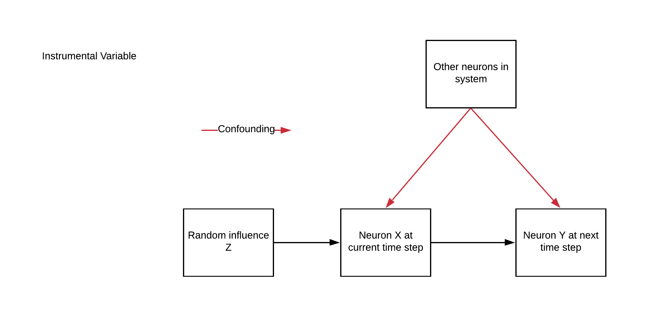
content_review(f"{feedback_prefix}_ IVs_in_simulated_neural_systems_Video")

さて、これまでシミュレーションしてきた神経系に、追加の変数 $\vec{z}$ があるとします。これが我々の操作変数（IV）となります。

$\vec{z}$ はニューロンのダイナミクスにおけるノイズの一種として扱います：

\vec{x}_{t+1} = \sigma(A\vec{x}_t + \eta \vec{z}_{t+1} + \epsilon_t)

$\eta$ はIVの「強さ」と呼ぶものです
$\vec{z}_t$ はランダムな二値変数で、 $\vec{z}_t \sim Bernoulli(0.5)$

各ニューロン $i$ について、我々は $i$ が次の時刻の他のニューロンに接続（因果的影響）しているかを調べています。つまり時刻 $t$ において、 $\vec{x}_{i,t}$ が $\vec{x}_{t+1}$ の他のニューロンに影響を与えているかを判定します。あるニューロン $i$ に対して、 $\vec{z}_{i,t}$ は有効な操作変数の3つの条件を満たします。

$z$ は生物学的には何を意味するのか？

$z$ は in vivo パッチクランプによる注入電流と考えてみてください。各ニューロンに個別に影響し、そのニューロンを通じてのみダイナミクスに影響を与えます。

IVの良いところは、 $z$ を自分で制御する必要がなく、観測できればよい点です。もし配線を間違えて注入電圧がAMラジオに繋がってしまっても問題ありません。信号を観測できさえすれば、この方法は機能します。

セクション 2.1: IVを用いたシステムのシミュレーション

コーディング演習 2.1: IVを用いたシステムのシミュレーション

ここでは神経系をシミュレートする関数を修正し、更新則に操作変数 $z$ の効果を含めます。

def simulate_neurons_iv(n_neurons, timesteps, eta, random_state=42):
  """
  Simulates a dynamical system for the specified number of neurons and timesteps.

  Args:
      n_neurons (int): the number of neurons in our system.
      timesteps (int): the number of timesteps to simulate our system.
      eta (float): the strength of the instrument
      random_state (int): seed for reproducibility

  Returns:
      The tuple (A,X,Z) of the connectivity matrix, simulated system, and instruments.
      - A has shape (n_neurons, n_neurons)
      - X has shape (n_neurons, timesteps)
      - Z has shape (n_neurons, timesteps)
  """
  np.random.seed(random_state)
  A = create_connectivity(n_neurons, random_state)

  X = np.zeros((n_neurons, timesteps))
  Z = np.random.choice([0, 1], size=(n_neurons, timesteps))
  for t in range(timesteps - 1):

    ############################################################################
    ## Insert your code here to adjust the update rule to include the
    ## instrumental variable.
    ##  We've already created Z for you. (We need to return it to regress on it).
    ##  Your task is to slice it appropriately. Don't forget eta.
    ## Fill out function and remove
    raise NotImplementedError('Complete simulate_neurons_iv function')
    ############################################################################

    IV_on_this_timestep = ...

    X[:, t + 1] = sigmoid(A.dot(X[:, t]) + IV_on_this_timestep + np.random.multivariate_normal(np.zeros(n_neurons), np.eye(n_neurons)))

  return A, X, Z


# Set parameters
timesteps = 5000  # Simulate for 5000 timesteps.
n_neurons = 100  # the size of our system
eta = 2  # the strength of our instrument, higher is stronger

# Simulate our dynamical system for the given amount of time
A, X, Z = simulate_neurons_iv(n_neurons, timesteps, eta)

# Visualize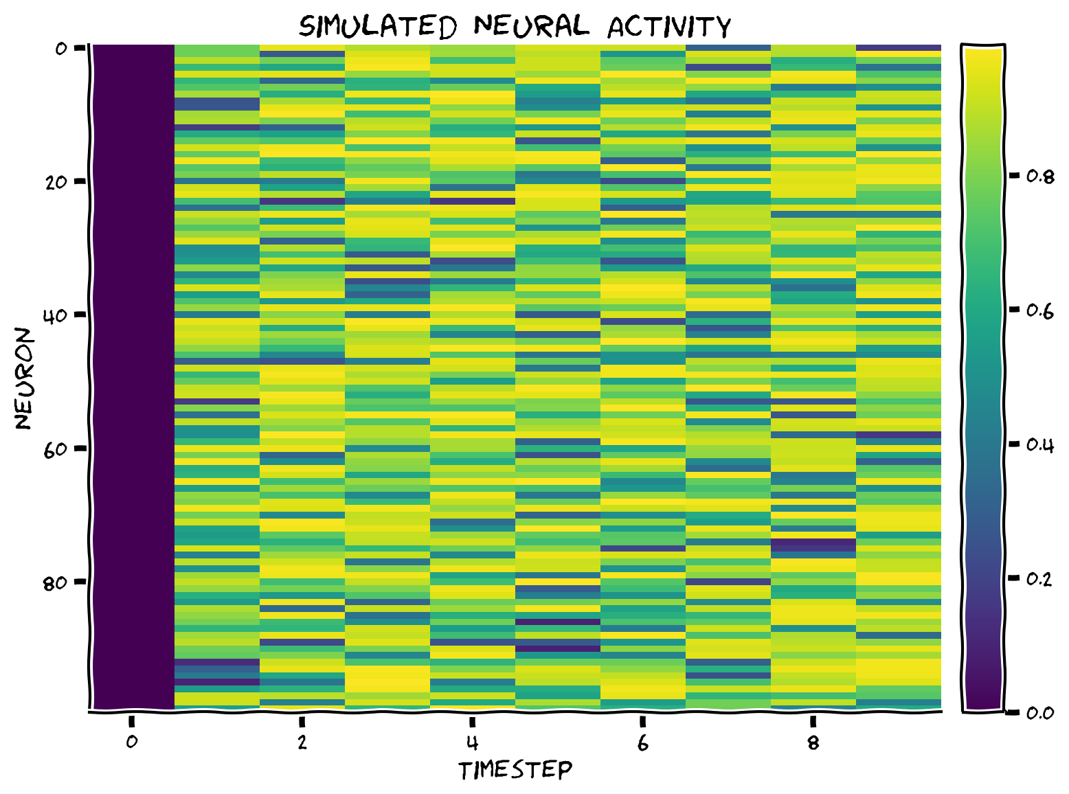
plot_neural_activity(X)

解答を見る$

出力例:

# @title Submit your feedback
content_review(f"{feedback_prefix}_Simulate_a_system_with_IV_Exercise")

セクション 2.2: シミュレーション神経系のIV推定

先ほど2段階最小二乗法を実装したので、ネットワークの実装は関数 $get_iv_estimate_network()$ として用意しました。では、IV推定が結合行列の回復にどの程度役立つか見てみましょう。

def get_iv_estimate_network(X, Z):
  """
  Estimates the connectivity matrix from 2-stage least squares regression
  using an instrument.

  Args:
      X (np.ndarray): our simulated system of shape (n_neurons, timesteps)
      Z (np.ndarray): our observed instruments of shape (n_neurons, timesteps)

  Returns:

      V (np.ndarray): the estimated connectivity matrix
  """
  n_neurons = X.shape[0]
  Y = X[:, 1:].transpose()

  # apply inverse sigmoid transformation
  Y = logit(Y)

  # Stage 1: regress X on Z
  stage1 = MultiOutputRegressor(LinearRegression(fit_intercept=True), n_jobs=-1)
  stage1.fit(Z[:, :-1].transpose(), X[:, :-1].transpose())
  X_hat = stage1.predict(Z[:, :-1].transpose())

  # Stage 2: regress Y on X_hatI
  stage2 = MultiOutputRegressor(LinearRegression(fit_intercept=True), n_jobs=-1)
  stage2.fit(X_hat, Y)

  # Get estimated effects
  V = np.zeros((n_neurons, n_neurons))
  for i, estimator in enumerate(stage2.estimators_):
    V[i, :] = estimator.coef_

  return V

では、私たちのシステムでどのくらいうまく機能するか見てみましょう。

# @markdown Execute this cell to visualize IV estimated connectivity matrix
n_neurons = 6
timesteps = 10000
random_state = 42
eta = 2

A, X, Z = simulate_neurons_iv(n_neurons, timesteps, eta, random_state)
V = get_iv_estimate_network(X, Z)
corr_ = np.corrcoef(A.flatten(), V.flatten())[1, 0]

fig, axs = plt.subplots(1, 2, figsize=(10, 5))

im = axs[0].imshow(A, cmap="coolwarm")
fig.colorbar(im, ax=axs[0],fraction=0.046, pad=0.04)
axs[0].title.set_text("True connectivity matrix")
axs[0].set(xlabel='Connectivity from', ylabel='Connectivity to')

im = axs[1].imshow(V, cmap="coolwarm")
fig.colorbar(im, ax=axs[1],fraction=0.046, pad=0.04)
axs[1].title.set_text("IV estimated connectivity matrix")
axs[1].set(xlabel='Connectivity from')
fig.suptitle(f"IV estimated correlation: {corr_:.3f}")
plt.show()

IV推定はかなりうまく機能しているようです！次のセクションでは、欠落変数バイアスに直面したときの挙動を見ていきます。

セクション 3: IVと欠落変数バイアス

チュートリアル開始からここまでの推定時間: 40分

# @title Video 5: IV vs regression
from ipywidgets import widgets
from IPython.display import YouTubeVideo
from IPython.display import IFrame
from IPython.display import display


class PlayVideo(IFrame):
  def __init__(self, id, source, page=1, width=400, height=300, **kwargs):
    self.id = id
    if source == 'Bilibili':
      src = f'https://player.bilibili.com/player.html?bvid={id}&page={page}'
    elif source == 'Osf':
      src = f'https://mfr.ca-1.osf.io/render?url=https://osf.io/download/{id}/?direct%26mode=render'
    super(PlayVideo, self).__init__(src, width, height, **kwargs)


def display_videos(video_ids, W=400, H=300, fs=1):
  tab_contents = []
  for i, video_id in enumerate(video_ids):
    out = widgets.Output()
    with out:
      if video_ids[i][0] == 'Youtube':
        video = YouTubeVideo(id=video_ids[i][1], width=W,
                             height=H, fs=fs, rel=0)
        print(f'Video available at https://youtube.com/watch?v={video.id}')
      else:
        video = PlayVideo(id=video_ids[i][1], source=video_ids[i][0], width=W,
                          height=H, fs=fs, autoplay=False)
        if video_ids[i][0] == 'Bilibili':
          print(f'Video available at https://www.bilibili.com/video/{video.id}')
        elif video_ids[i][0] == 'Osf':
          print(f'Video available at https://osf.io/{video.id}')
      display(video)
    tab_contents.append(out)
  return tab_contents


video_ids = [('Youtube', 'zceWyoQn09s'), ('Bilibili', 'BV1pv411q7Hc')]
tab_contents = display_videos(video_ids, W=854, H=480)
tabs = widgets.Tab()
tabs.children = tab_contents
for i in range(len(tab_contents)):
  tabs.set_title(i, video_ids[i][0])
display(tabs)

# @title Submit your feedback
content_review(f"{feedback_prefix}_IVs_and_omitted_variable_bias_Video")

インタラクティブデモ 3: 観測神経細胞のサブセットに対するIVと回帰による結合推定

観測神経細胞の割合を変えて、IVと回帰による結合推定の品質への影響を見てみましょう。観測神経細胞が少ない場合、どちらの方法がより良い結果を出すでしょうか？

# @markdown Execute this cell to enable the widget.

# @markdown This simulation will take about a minute to run!

n_neurons = 30
timesteps = 20000
random_state = 42
eta = 2
A, X, Z = simulate_neurons_iv(n_neurons, timesteps, eta, random_state)

reg_args = {
    "fit_intercept": False,
    "alpha": 0.001
}

@widgets.interact
def plot_observed(ratio=[0.2, 0.4, 0.6, 0.8, 1.0]):
  fig, axs = plt.subplots(1, 3, figsize=(15, 5))
  sel_idx = int(ratio * n_neurons)
  n_observed = sel_idx
  offset = np.zeros((n_neurons, n_neurons))
  offset[:sel_idx, :sel_idx] =  1 + A[:sel_idx, :sel_idx]
  im = axs[0].imshow(offset, cmap="coolwarm", vmin=0, vmax=A.max() + 1)
  axs[0].title.set_text("True connectivity")
  axs[0].set_xlabel("Connectivity to")
  axs[0].set_ylabel("Connectivity from")
  plt.colorbar(im, ax=axs[0],fraction=0.046, pad=0.04)

  sel_A = A[:sel_idx, :sel_idx]
  sel_X = X[:sel_idx, :]
  sel_Z = Z[:sel_idx, :]

  V = get_iv_estimate_network(sel_X, sel_Z)
  iv_corr = np.corrcoef(sel_A.flatten(), V.flatten())[1, 0]

  big_V = np.zeros(A.shape)
  big_V[:sel_idx, :sel_idx] =  1 + V

  im = axs[1].imshow(big_V, cmap="coolwarm", vmin=0, vmax=A.max() + 1)
  plt.colorbar(im, ax=axs[1], fraction=0.046, pad=0.04)
  c = 'w' if n_observed < (n_neurons - 3) else 'k'
  axs[1].text(0, n_observed + 2, f"Correlation: {iv_corr:.2f}",
              color=c, size=15)
  axs[1].axis("off")


  reg_corr, R = get_regression_corr_full_connectivity(n_neurons, A, X, ratio,
                                                      reg_args)


  big_R = np.zeros(A.shape)
  big_R[:sel_idx, :sel_idx] =  1 + R

  im = axs[2].imshow(big_R, cmap="coolwarm", vmin=0, vmax=A.max() + 1)
  plt.colorbar(im, ax=axs[2], fraction=0.046, pad=0.04)
  c = 'w' if n_observed<(n_neurons-3) else 'k'
  axs[1].title.set_text("Estimated connectivity (IV)")
  axs[1].set_xlabel("Connectivity to")
  axs[1].set_ylabel("Connectivity from")

  axs[2].text(0, n_observed + 2, f"Correlation: {reg_corr:.2f}",
              color=c, size=15)
  axs[2].axis("off")
  axs[2].title.set_text("Estimated connectivity (regression)")
  axs[2].set_xlabel("Connectivity to")
  axs[2].set_ylabel("Connectivity from")
  plt.show()

以下で、観測神経細胞の割合に対する回帰とIVの性能を可視化することもできます。

注意このコードは実行に約1分かかります！

# @markdown Execute this cell to visualize connectivity estimation performance
def compare_iv_estimate_to_regression(observed_ratio):
  """
  A wrapper function to compare IV and Regressor performance as a function of
  observed neurons

  Args:
    observed_ratio(list): a list of different observed ratios
    (out of the whole system)
  """
  # Let's compare IV estimates to our regression estimates
  reg_corrs = np.zeros((len(observed_ratio),))
  iv_corrs = np.zeros((len(observed_ratio),))
  for j, ratio in enumerate(observed_ratio):
    sel_idx = int(ratio * n_neurons)

    sel_X = X[:sel_idx, :]
    sel_Z = X[:sel_idx, :]
    sel_A = A[:sel_idx, :sel_idx]

    sel_reg_V = get_regression_estimate(sel_X)
    reg_corrs[j] = np.corrcoef(sel_A.flatten(), sel_reg_V.flatten())[1, 0]

    sel_iv_V = get_iv_estimate_network(sel_X, sel_Z)
    iv_corrs[j] = np.corrcoef(sel_A.flatten(), sel_iv_V.flatten())[1, 0]

  # Plotting IV vs lasso performance
  plt.plot(observed_ratio, reg_corrs)
  plt.plot(observed_ratio, iv_corrs)
  plt.xlim([1, 0.2])
  plt.ylabel("Connectivity matrices\ncorrelation with truth")
  plt.xlabel("Fraction of observed variables")
  plt.title("IV and lasso performance as a function of observed neuron ratio")
  plt.legend(['Regression', 'IV'])
  plt.show()


n_neurons = 40  # the size of the system
timesteps = 20000
random_state = 42
eta = 2  # the strength of our instrument

A, X, Z = simulate_neurons_iv(n_neurons, timesteps, eta, random_state)

observed_ratio = [1, 0.8, 0.6, 0.4, 0.2]

compare_iv_estimate_to_regression(observed_ratio)

IVは欠落変数バイアス（強いインストゥルメントがあり十分なデータがある場合）をうまく扱うことがわかります。

IV解析のコスト

適切で有効なインストゥルメントを見つける必要がある
2段階推定プロセスのため、強いインストゥルメントが必要で、そうでないと標準誤差が大きくなる

# @title Submit your feedback
content_review(f"{feedback_prefix}_Estimating_connectivity_with_IV_vs_regression_Interactive_Demo")

セクション 4: 自分の研究における因果性について考える

チュートリアル開始からここまでの推定時間: 50分

Think 4!: ディスカッションの質問

以下についてグループで約10分間話し合ってください。

最近の研究を振り返ってみてください。基本的な問いの因果図を作成できますか？因果妥当性に脅威となるバイアス（欠落変数やその他のもの）はありますか？
インストゥルメンタル変数の可能性を考えられますか？あなたの分野の研究で因果効果の特定に利用できる観測されたランダム性の源は何でしょうか？

# @title Submit your feedback
content_review(f"{feedback_prefix}_ Discussion_questions_Discussion")

まとめ

チュートリアルの推定所要時間: 1時間5分

# @title Video 6: Summary
from ipywidgets import widgets
from IPython.display import YouTubeVideo
from IPython.display import IFrame
from IPython.display import display


class PlayVideo(IFrame):
  def __init__(self, id, source, page=1, width=400, height=300, **kwargs):
    self.id = id
    if source == 'Bilibili':
      src = f'https://player.bilibili.com/player.html?bvid={id}&page={page}'
    elif source == 'Osf':
      src = f'https://mfr.ca-1.osf.io/render?url=https://osf.io/download/{id}/?direct%26mode=render'
    super(PlayVideo, self).__init__(src, width, height, **kwargs)


def display_videos(video_ids, W=400, H=300, fs=1):
  tab_contents = []
  for i, video_id in enumerate(video_ids):
    out = widgets.Output()
    with out:
      if video_ids[i][0] == 'Youtube':
        video = YouTubeVideo(id=video_ids[i][1], width=W,
                             height=H, fs=fs, rel=0)
        print(f'Video available at https://youtube.com/watch?v={video.id}')
      else:
        video = PlayVideo(id=video_ids[i][1], source=video_ids[i][0], width=W,
                          height=H, fs=fs, autoplay=False)
        if video_ids[i][0] == 'Bilibili':
          print(f'Video available at https://www.bilibili.com/video/{video.id}')
        elif video_ids[i][0] == 'Osf':
          print(f'Video available at https://osf.io/{video.id}')
      display(video)
    tab_contents.append(out)
  return tab_contents


video_ids = [('Youtube', '1qxW8CPW77U'), ('Bilibili', 'BV1Gt4y1X76z')]
tab_contents = display_videos(video_ids, W=854, H=480)
tabs = widgets.Tab()
tabs.children = tab_contents
for i in range(len(tab_contents)):
  tabs.set_title(i, video_ids[i][0])
display(tabs)

# @title Submit your feedback
content_review(f"{feedback_prefix}_Summary_Video")

このチュートリアルでは、

インストゥルメンタル変数とそれを因果推定に使う方法を探りました
IV推定と回帰推定を比較しました

ボーナス

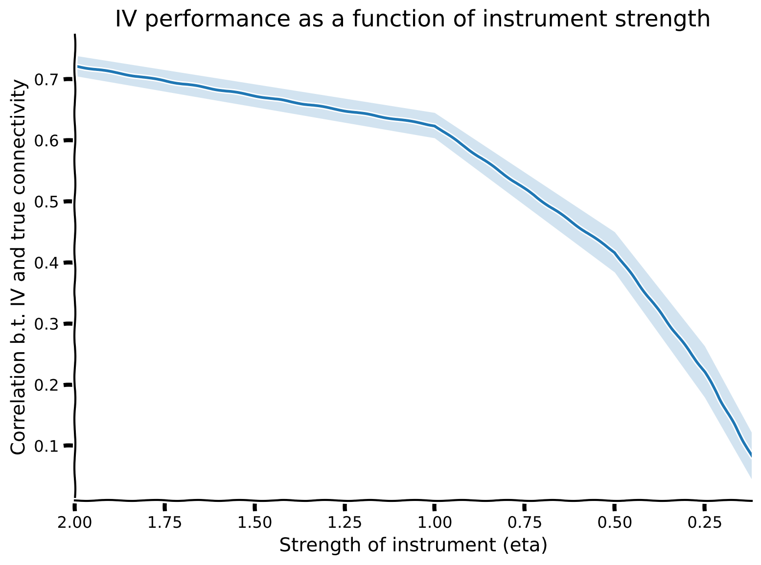
ボーナスセクション 1: インストゥルメントの強さを探る

ボーナスコーディング演習 1: インストゥルメントの強さを探る

インストゥルメント $\eta$ の強さがインストゥルメンタル変数推定の品質にどう影響するかを探ります。

def instrument_strength_effect(etas, n_neurons, timesteps, n_trials):
  """ Compute IV estimation performance for different instrument strengths

  Args:
    etas (list): different instrument strengths to compare
    n_neurons (int): number of neurons in simulation
    timesteps (int): number of timesteps in simulation
    n_trials (int): number of trials to compute

  Returns:
    ndarray: n_trials x len(etas) array where each element is the correlation
             between true and estimated connectivity matrices for that trial and
             instrument strength
  """

  # Initialize corr array
  corr_data = np.zeros((n_trials, len(etas)))

  # Loop over trials
  for trial in range(n_trials):
    print(f"simulation of trial {trial + 1} of {n_trials}")

    # Loop over instrument strengths
    for j, eta in enumerate(etas):
      ########################################################################
      ## TODO: Simulate system with a given instrument strength, get IV estimate,
      ## and compute correlation
      # Fill out function and remove
      raise NotImplementedError('Student exercise: complete instrument_strength_effect')
      ########################################################################

      # Simulate system
      A, X, Z = simulate_neurons_iv(...)

      # Compute IV estimate
      iv_V = get_iv_estimate_network(...)

      # Compute correlation
      corr_data[trial, j] =  np.corrcoef(A.flatten(), iv_V.flatten())[1, 0]

  return corr_data


# Parameters of system
n_neurons = 20
timesteps = 10000
n_trials = 3
etas = [2, 1, 0.5, 0.25, 0.12]  # instrument strengths to search over

# Get IV estimate performances
corr_data = instrument_strength_effect(etas, n_neurons, timesteps, n_trials)

# Visualize
plot_performance_vs_eta(etas, corr_data)

解答を見る$

出力例:

# @title Submit your feedback
content_review(f"{feedback_prefix}_Exploring_instrument_strength_Bonus_Exercise")

ボーナスセクション 2: グレンジャー因果性

時間的因果関係の別の可能な解決策として、グレンジャー因果性を考えます。

しかし、チュートリアル3で探った同時フィッティングと同様に、この方法も観測されていない変数がある場合には失敗します。

時系列 $X$ が時系列 $Y$ にグレンジャー因果するかどうかを仮説検定で調べます:

帰無仮説 $H_0$ : $X$ の遅延値は $Y$ の予測に役立たない
対立仮説 $H_a$ : $X$ の遅延値は $Y$ の予測に役立つ

機械的には、 $y_t$ の自己回帰モデルをフィットさせます。回帰で $x_{t-k}$ の項が有意に残らなければ帰無仮説を棄却できません。簡単のため、1つの時刻遅れのみ考えます。すなわち:

\begin{align}
H_0: $y_t$ &= $a_0$ + $a_1$ $y_{t-1}$ + $\epsilon_t$ \
H_a: $y_t$ &= $a_0$ + $a_1$ $y_{t-1}$ + $b_1$ $x_{t-1}$ + $\epsilon_t \end{align}$

# @markdown Execute this cell to get custom imports from [statsmodels](https://www.statsmodels.org/stable/index.html) library
from statsmodels.tsa.stattools import grangercausalitytests

ボーナスセクション 2.1: 小規模システムでのグレンジャー因果性

まず小規模システムでグレンジャー因果性を評価します。

ボーナスコーディング演習 2.1: グレンジャー因果性の評価

以下の定義を完成させて、ニューロン間のグレンジャー因果性を評価してください。その後、下のセルを実行してどの程度うまく機能するか評価します。statsmodels からすでにインポートされている grangercausalitytests() 関数を使います。小規模システムのニューロンが他のニューロンにグレンジャー因果するかを確認します。

def get_granger_causality(X, selected_neuron, alpha=0.05):
  """
  Estimates the lag-1 granger causality of the given neuron on the other neurons in the system.

  Args:
      X (np.ndarray): the matrix holding our dynamical system of shape (n_neurons, timesteps)
      selected_neuron (int): the index of the neuron we want to estimate granger causality for
      alpha (float): Bonferroni multiple comparisons correction

  Returns:
      A tuple (reject_null, p_vals)
      reject_null (list): a binary list of length n_neurons whether the null was
          rejected for the selected neuron granger causing the other neurons
      p_vals (list): a list of the p-values for the corresponding Granger causality tests
  """
  n_neurons = X.shape[0]
  max_lag = 1

  reject_null = []
  p_vals = []

  for target_neuron in range(n_neurons):
    ts_data = X[[target_neuron, selected_neuron], :].transpose()

    ########################################################################
    ## Insert your code here to run Granger causality tests.
    ##
    ## Function Hints:
    ##     Pass the ts_data defined above as the first argument
    ##     Granger causality -> grangercausalitytests
    ## Fill out this function and then remove
    raise NotImplementedError('Student exercise: complete get_granger_causality function')
    ########################################################################
    res = grangercausalitytests(...)

    # Gets the p-value for the log-ratio test
    pval = res[1][0]['lrtest'][1]

    p_vals.append(pval)
    reject_null.append(int(pval < alpha))

  return reject_null, p_vals


# Set up small system
n_neurons = 6
timesteps = 5000
random_state = 42
selected_neuron = 1

A = create_connectivity(n_neurons, random_state)
X = simulate_neurons(A, timesteps, random_state)

# Estimate Granger causality
reject_null, p_vals = get_granger_causality(X, selected_neuron)

# Visualize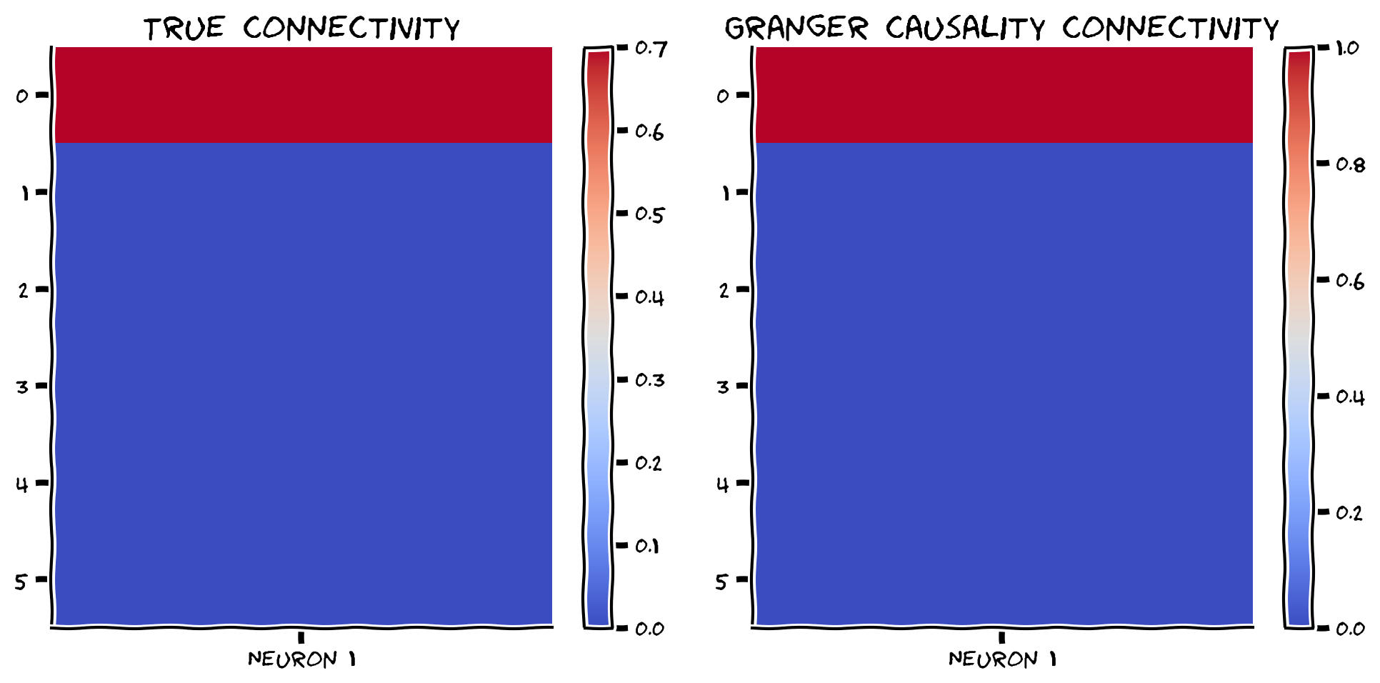
compare_granger_connectivity(A, reject_null, selected_neuron)

解答を見る$

出力例:

# @title Submit your feedback
content_review(f"{feedback_prefix}_Evaluate_Granger_causality_Bonus_Exercise")

良さそうです！グレンジャー推定と真の結合の相関も確認しましょう。

print(np.corrcoef(A[:, selected_neuron], np.array(reject_null))[1, 0])

小規模システムでは、ニューロン1の因果性を正しく特定できています。

ボーナスセクション 2.2: 大規模システムでのグレンジャー因果性

次に100ニューロンの大規模システムでグレンジャー因果性を実行します。まだうまく機能するでしょうか？タイムステップ数はどう影響するでしょうか？

# @markdown Execute this cell to examine Granger causality in a large system
n_neurons = 100
timesteps = 5000
random_state = 42
selected_neuron = 1
A = create_connectivity(n_neurons, random_state)
X = simulate_neurons(A, timesteps, random_state)

# get granger causality estimates
reject_null, p_vals = get_granger_causality(X, selected_neuron)
compare_granger_connectivity(A, reject_null, selected_neuron)

再びグレンジャー推定と真の結合の相関を確認しましょう。この大規模システムで真の結合をうまく回復できているでしょうか？

print(np.corrcoef(A[:, selected_neuron], np.array(reject_null))[1, 0])

グレンジャー因果性に関する注意点

ここでは2変数間のグレンジャー因果性を考えました。すなわち、ニューロンペア $A, B$ について、一方が他方にグレンジャー因果するかを調べました。より多くの変数を考慮すると推定が改善されるかもしれません。条件付きグレンジャー因果性は多変量システムに対応し、他の変数を条件にして $A$ が $B$ にグレンジャー因果するかを検定します。

しかし、システム内の変数を制御しても、システムが大きくなると条件付きグレンジャー因果性も性能が悪くなる可能性があります。さらに、条件付けに必要な追加変数の測定が実際には困難であり、回帰演習で見たように欠落変数バイアスを生じることがあります。

ここからの教訓は、推定手法が高度になるほど解釈が難しくなることです。常に手法とその仮定を理解する必要があります。

チュートリアル 4: 器具変数（Instrumental Variables）

チュートリアルの目的

セットアップ

セクション1: 器具変数（Instrumental Variables）

セクション1.1: 器具変数の非神経科学的な例

セクション1.2: 器具変数の仕組み（概要）

セクション1.3: 2段階最小二乗法によるIV推定

セクション 1.3.1: 最小二乗回帰 ステージ1

コーディング演習 1.3.1: 回帰ステージ1の計算

提案

セクション 1.3.2: 最小二乗回帰 ステージ2

コーディング演習 1.3.2: IV推定量の計算

セクション 2: シミュレーションした神経系におけるIV

セクション 2.1: IVを用いたシステムのシミュレーション

コーディング演習 2.1: IVを用いたシステムのシミュレーション

セクション 2.2: シミュレーション神経系のIV推定

セクション 3: IVと欠落変数バイアス

インタラクティブデモ 3: 観測神経細胞のサブセットに対するIVと回帰による結合推定

セクション 4: 自分の研究における因果性について考える

Think 4!: ディスカッションの質問

まとめ

ボーナス

ボーナスセクション 1: インストゥルメントの強さを探る

ボーナスコーディング演習 1: インストゥルメントの強さを探る

ボーナスセクション 2: グレンジャー因果性

ボーナスセクション 2.1: 小規模システムでのグレンジャー因果性

ボーナスコーディング演習 2.1: グレンジャー因果性の評価

ボーナスセクション 2.2: 大規模システムでのグレンジャー因果性

セクション 1.3.1: 最小二乗回帰ステージ1

セクション 1.3.2: 最小二乗回帰ステージ2