チュートリアル 2: 相関

第3週5日目: ネットワーク因果性

Neuromatch Academyによる

コンテンツ作成者: アリ・ベンジャミン、トニー・リウ、コンラッド・コーディング

コンテンツレビュアー: マイク・X・コーエン、マディネ・サルヴェスタニ、ヨニ・フリードマン、エラ・バティ、マイケル・ワスコム

制作編集者: ガガナ・B、スピロス・チャヴリス

チュートリアルの目的

チュートリアルの推定所要時間: 45分

これは因果性を検証する日のチュートリアル2です。以下は本日扱う内容の大まかな概要で、今回のチュートリアルで重点的に扱うセクションは太字にしています:

因果性の定義をマスターする
因果性の推定が可能であることを理解する
4つの異なる方法を学び、それらが失敗する場合を理解する

介入（摂動）
相関
同時フィッティング／回帰
器具変数法

チュートリアル2の目的

チュートリアル1では、本日扱うニューロンの動的システムを実装し、探索しました。また、ランダムな摂動による因果効果の測定という「ゴールドスタンダード」について学びました。ランダム摂動がしばしば不可能なため、今回は因果性を測定しようとする代替手法に目を向けます。以下を行います:

相関が因果を近似すると仮定して、観察から結合性を推定する方法を学ぶ
これはネットワークが小さい場合にのみ有効であることを示す

チュートリアル2の設定

多くの場合、神経活動や脳領域を強制的にオン・オフにできません。観察するしかありません。2つのノード間の相関を得られたとして、それは十分でしょうか？このチュートリアルで問うのは、**相関が因果の「十分な」代替となるのはいつか？**ということです。

答えは「決してない」ではなく、「場合によってはある」ということです。

# @title Tutorial slides
# @markdown These are the slides for the videos in all tutorials today
from IPython.display import IFrame
link_id = "gp4m9"
print(f"If you want to download the slides: https://osf.io/download/{link_id}/")
IFrame(src=f"https://mfr.ca-1.osf.io/render?url=https://osf.io/{link_id}/?direct%26mode=render%26action=download%26mode=render", width=854, height=480)

セットアップ

# @title Install and import feedback gadget


from vibecheck import DatatopsContentReviewContainer
def content_review(notebook_section: str):
    return DatatopsContentReviewContainer(
        "",  # No text prompt
        notebook_section,
        {
            "url": "https://pmyvdlilci.execute-api.us-east-1.amazonaws.com/klab",
            "name": "neuromatch_cn",
            "user_key": "y1x3mpx5",
        },
    ).render()


feedback_prefix = "W3D5_T2"

# Imports
import numpy as np
import matplotlib.pyplot as plt

# @title Figure Settings
import logging
logging.getLogger('matplotlib.font_manager').disabled = True

import ipywidgets as widgets  # interactive display
%config InlineBackend.figure_format = 'retina'
plt.style.use("https://raw.githubusercontent.com/NeuromatchAcademy/course-content/main/nma.mplstyle")

# @title Plotting Functions

def see_neurons(A, ax, show=False):
  """
  Visualizes the connectivity matrix.

  Args:
      A (np.ndarray): the connectivity matrix of shape (n_neurons, n_neurons)
      ax (plt.axis): the matplotlib axis to display on

  Returns:
      Nothing, but visualizes A.
  """
  A = A.T  # make up for opposite connectivity
  n = len(A)
  ax.set_aspect('equal')
  thetas = np.linspace(0, np.pi * 2, n, endpoint=False)
  x, y = np.cos(thetas), np.sin(thetas),
  ax.scatter(x, y, c='k', s=150)
  A = A / A.max()
  for i in range(n):
    for j in range(n):
      if A[i, j] > 0:
        ax.arrow(x[i], y[i], x[j] - x[i], y[j] - y[i],
                 color='k', alpha=A[i, j], head_width=.15,
                 width = A[i,j] / 25, shape='right',
                 length_includes_head=True)
  ax.axis('off')
  if show:
    plt.show()


def plot_estimation_quality_vs_n_neurons(number_of_neurons):
  """
  A wrapper function that calculates correlation between true and estimated connectivity
  matrices for each number of neurons and plots

  Args:
    number_of_neurons (list): list of different number of neurons for modeling system
    corr_func (function): Function for computing correlation
  """
  corr_data = np.zeros((n_trials, len(number_of_neurons)))
  for trial in range(n_trials):
    print(f"simulating trial {trial + 1} of {n_trials}")
    for j, size in enumerate(number_of_neurons):
      corr = get_sys_corr(size, timesteps, trial)
      corr_data[trial, j] = corr

  corr_mean = corr_data.mean(axis=0)
  corr_std = corr_data.std(axis=0)

  plt.figure()
  plt.plot(number_of_neurons, corr_mean)
  plt.fill_between(number_of_neurons, corr_mean - corr_std,
                   corr_mean + corr_std, alpha=.2)
  plt.xlabel("Number of neurons")
  plt.ylabel("Correlation")
  plt.title("Similarity between A and R as a function of network size")
  plt.show()


def plot_connectivity_matrix(A, ax=None, show=False):
  """Plot the (weighted) connectivity matrix A as a heatmap

    Args:
      A (ndarray): connectivity matrix (n_neurons by n_neurons)
      ax: axis on which to display connectivity matrix
  """
  if ax is None:
    ax = plt.gca()
  lim = np.abs(A).max()
  im = ax.imshow(A, vmin=-lim, vmax=lim, cmap="coolwarm")
  ax.tick_params(labelsize=10)
  ax.xaxis.label.set_size(15)
  ax.yaxis.label.set_size(15)
  cbar = ax.figure.colorbar(im, ax=ax, ticks=[0], shrink=.7)
  cbar.ax.set_ylabel("Connectivity Strength", rotation=90,
                     labelpad=20, va="bottom")
  ax.set(xlabel="Connectivity from", ylabel="Connectivity to")
  if show:
    plt.show()


def plot_true_vs_estimated_connectivity(estimated_connectivity,
                                        true_connectivity,
                                        selected_neuron=None,
                                        correlation=None):
  """Visualize true vs estimated connectivity matrices

  Args:
    estimated_connectivity (ndarray): estimated connectivity (n_neurons by n_neurons)
    true_connectivity (ndarray): ground-truth connectivity (n_neurons by n_neurons)
    correlation (float): correlation between true and estimated connectivity
    selected_neuron (int or None): None if plotting all connectivity, otherwise connectivity
      from selected_neuron will be shown

  """
  fig, axs = plt.subplots(1, 2, figsize=(10, 5))

  if selected_neuron is not None:
    plot_connectivity_matrix(true_connectivity[:, [selected_neuron]], ax=axs[0])
    plot_connectivity_matrix(np.expand_dims(estimated_connectivity, axis=1),
                             ax=axs[1])
    axs[0].set_xticks([0])
    axs[1].set_xticks([0])
    axs[0].set_xticklabels([selected_neuron])
    axs[1].set_xticklabels([selected_neuron])
  else:
    plot_connectivity_matrix(true_connectivity, ax=axs[0])
    plot_connectivity_matrix(estimated_connectivity, ax=axs[1])

  axs[0].set(title="True connectivity matrix A")
  axs[1].set(title="Estimated connectivity matrix R")
  if correlation:
    fig.suptitle(f"Correlation between A and R: {correlation:.3f}")
  plt.show()

# @title Helper Functions

def sigmoid(x):
  """
  Compute sigmoid nonlinearity element-wise on x.

  Args:
    x (np.ndarray): the numpy data array we want to transform
  Returns
    (np.ndarray): x with sigmoid nonlinearity applied
  """
  return 1 / (1 + np.exp(-x))


def create_connectivity(n_neurons, random_state=42, p=0.9):
  """
  Generate our nxn causal connectivity matrix.

  Args:
    n_neurons (int): the number of neurons in our system.
    random_state (int): random seed for reproducibility

  Returns:
    A (np.ndarray): our 0.1 sparse connectivity matrix
  """
  np.random.seed(random_state)
  A_0 = np.random.choice([0, 1], size=(n_neurons, n_neurons), p=[p, 1 - p])

  # set the timescale of the dynamical system to about 100 steps
  _, s_vals, _ = np.linalg.svd(A_0)
  if s_vals[0] != 0 and not np.isnan(s_vals[0]):
    A = A_0 / (1.01 * s_vals[0])
  else:
    eps = 1e-12
    A = eps*np.ones_like(A_0)  # if denominator is zero, set A to a small value

  return A


def simulate_neurons(A, timesteps, random_state=42):
  """
  Simulates a dynamical system for the specified number of neurons and timesteps.

  Args:
    A (np.array): the connectivity matrix
    timesteps (int): the number of timesteps to simulate our system.
    random_state (int): random seed for reproducibility

  Returns:
    X has shape (n_neurons, timeteps).
  """
  np.random.seed(random_state)
  n_neurons = len(A)
  X = np.zeros((n_neurons, timesteps))

  for t in range(timesteps - 1):
    epsilon = np.random.multivariate_normal(np.zeros(n_neurons),
                                            np.eye(n_neurons))
    X[:, t + 1] = sigmoid(A.dot(X[:, t]) + epsilon)

  return X


def get_sys_corr(n_neurons, timesteps, random_state=42, neuron_idx=None):
  """
  A wrapper function for our correlation calculations between A and R.

  Args:
    n_neurons (int): the number of neurons in our system.
    timesteps (int): the number of timesteps to simulate our system.
    random_state (int): seed for reproducibility
    neuron_idx (int): optionally provide a neuron idx to slice out

  Returns:
    A single float correlation value representing the similarity between A and R
  """
  A = create_connectivity(n_neurons, random_state)
  X = simulate_neurons(A, timesteps)
  R = correlation_for_all_neurons(X)

  return np.corrcoef(A.flatten(), R.flatten())[0, 1]

上で定義したヘルパー関数は以下の通りです:

sigmoid: チュートリアル1からの、入力に対して要素ごとにシグモイド非線形変換を計算する関数。
create_connectivity: チュートリアル1からの、nxnの因果結合行列を生成する関数。
simulate_neurons: チュートリアル1からの、指定したニューロン数とタイムステップ数で動的システムをシミュレートする関数。
get_sys_corr: $A$ と $R$ 間の相関計算のラッパー関数。

セクション1: 小規模システム

# @title Video 1: Correlation vs causation
from ipywidgets import widgets
from IPython.display import YouTubeVideo
from IPython.display import IFrame
from IPython.display import display


class PlayVideo(IFrame):
  def __init__(self, id, source, page=1, width=400, height=300, **kwargs):
    self.id = id
    if source == 'Bilibili':
      src = f'https://player.bilibili.com/player.html?bvid={id}&page={page}'
    elif source == 'Osf':
      src = f'https://mfr.ca-1.osf.io/render?url=https://osf.io/download/{id}/?direct%26mode=render'
    super(PlayVideo, self).__init__(src, width, height, **kwargs)


def display_videos(video_ids, W=400, H=300, fs=1):
  tab_contents = []
  for i, video_id in enumerate(video_ids):
    out = widgets.Output()
    with out:
      if video_ids[i][0] == 'Youtube':
        video = YouTubeVideo(id=video_ids[i][1], width=W,
                             height=H, fs=fs, rel=0)
        print(f'Video available at https://youtube.com/watch?v={video.id}')
      else:
        video = PlayVideo(id=video_ids[i][1], source=video_ids[i][0], width=W,
                          height=H, fs=fs, autoplay=False)
        if video_ids[i][0] == 'Bilibili':
          print(f'Video available at https://www.bilibili.com/video/{video.id}')
        elif video_ids[i][0] == 'Osf':
          print(f'Video available at https://osf.io/{video.id}')
      display(video)
    tab_contents.append(out)
  return tab_contents


video_ids = [('Youtube', 'vjBO-S7KNPI'), ('Bilibili', 'BV1Ak4y1m7kk')]
tab_contents = display_videos(video_ids, W=854, H=480)
tabs = widgets.Tab()
tabs.children = tab_contents
for i in range(len(tab_contents)):
  tabs.set_title(i, video_ids[i][0])
display(tabs)

# @title Submit your feedback
content_review(f"{feedback_prefix}_Correlation_vs_causation_Video")

コーディング演習1: 相関で因果を近似してみよう

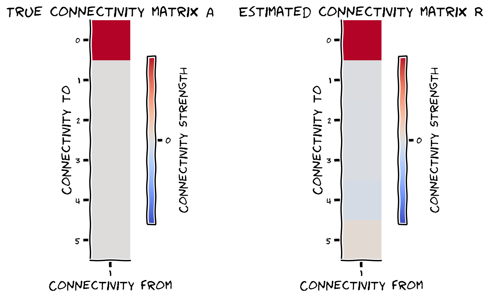
小規模システムでは、相関が因果のように見えることがあります。各タイムステップの神経状態と前の状態の相関を取るだけで、真の結合行列 ( $A$ ) を復元してみましょう: $C = \vec{x_t} \vec{x_{t+1}}^\top$ 。

この関数を完成させて、単一ニューロンの結合行列を推定してください。具体的には、選択したニューロンの時刻 $t$ の活動と、他のすべてのニューロンの時刻 $t+1$ の活動の相関係数を計算します。つまり、2つのベクトルの相関を計算してください:

選択したニューロンの時刻 $t$ の活動
すべての他のニューロンの時刻 $t+1$ の活動

def compute_connectivity_from_single_neuron(X, selected_neuron):
  """
  Computes the connectivity matrix from a single neuron neurons using correlations

  Args:
      X (ndarray): the matrix of activities
      selected_neuron (int): the index of the selected neuron

  Returns:
      estimated_connectivity (ndarray): estimated connectivity for the selected neuron, of shape (n_neurons,)
  """

  # Extract the current activity of selected_neuron, t
  current_activity = X[selected_neuron, :-1]

  # Extract the observed outcomes of all the neurons
  next_activity = X[:, 1:]

  # Initialize estimated connectivity matrix
  estimated_connectivity = np.zeros(n_neurons)

  # Loop through all neurons
  for neuron_idx in range(n_neurons):

    # Get the activity of neuron_idx
    this_output_activity = next_activity[neuron_idx]

    ########################################################################
    ## TODO: Estimate the neural correlations between
    ## this_output_activity        and       current_activity
    ## -------------------                  ----------------
    ##
    ## Note that np.corrcoef returns the full correlation matrix; we want the
    ## top right corner, which we have already provided.
    ## FIll out function and remove
    raise NotImplementedError('Compute neural correlations')
    ########################################################################
    # Compute correlation
    correlation = np.corrcoef(...)[0, 1]

    # Store this neuron's correlation
    estimated_connectivity[neuron_idx] = correlation

  return estimated_connectivity


# Simulate a 6 neuron system for 5000 timesteps again.
n_neurons = 6
timesteps = 5000
selected_neuron = 1

# Invoke a helper function that generates our nxn causal connectivity matrix
A = create_connectivity(n_neurons)

# Invoke a helper function that simulates the neural activity
X = simulate_neurons(A, timesteps)

# Estimate connectivity
estimated_connectivity = compute_connectivity_from_single_neuron(X, selected_neuron)

# Visualize
plot_true_vs_estimated_connectivity(estimated_connectivity, A, selected_neuron)

解答を見る$

出力例:

# @title Submit your feedback
content_review(f"{feedback_prefix}_Approximate_causation_with_correlation_Exercise")

うまくいったのが見えたでしょうか。あなたがやったことを行列形式で実装した関数も用意しました。これにより少し高速になり、すべてのニューロンを同時に処理できます（ヘルパー関数 correlation_for_all_neurons）。

# @markdown Execute this cell get helper function `correlation_for_all_neurons`

def correlation_for_all_neurons(X):
  """Computes the connectivity matrix for the all neurons using correlations

    Args:
        X: the matrix of activities

    Returns:
        estimated_connectivity (np.ndarray): estimated connectivity for the selected neuron, of shape (n_neurons,)
  """
  n_neurons = len(X)
  S = np.concatenate([X[:, 1:], X[:, :-1]], axis=0)
  R = np.corrcoef(S)[:n_neurons, n_neurons:]
  return R

# @markdown Execute this cell to visualize full estimated vs true connectivity

R = correlation_for_all_neurons(X)

fig, axs = plt.subplots(2, 2, figsize=(10, 10))
see_neurons(A, axs[0, 0])
plot_connectivity_matrix(A, ax=axs[0, 1])
axs[0, 1].set_title("True connectivity matrix A")

see_neurons(R, axs[1, 0])
plot_connectivity_matrix(R, ax=axs[1, 1])
axs[1, 1].set_title("Estimated connectivity matrix R")

fig.suptitle("True (A) and Estimated (R) connectivity matrices")

plt.tight_layout()
plt.show()

これもほぼうまくいきました。どの程度うまくいったか定量化しましょう。

真の結合行列と推定行列の相関係数を計算します。

print(f"Correlation matrix of A and R: {np.corrcoef(A.flatten(), R.flatten())[0, 1]:.5f}")

我々のシステムでは、相関が因果を捉えているように見えます。

# @title Video 2: Correlation ~ causation for small systems
from ipywidgets import widgets
from IPython.display import YouTubeVideo
from IPython.display import IFrame
from IPython.display import display


class PlayVideo(IFrame):
  def __init__(self, id, source, page=1, width=400, height=300, **kwargs):
    self.id = id
    if source == 'Bilibili':
      src = f'https://player.bilibili.com/player.html?bvid={id}&page={page}'
    elif source == 'Osf':
      src = f'https://mfr.ca-1.osf.io/render?url=https://osf.io/download/{id}/?direct%26mode=render'
    super(PlayVideo, self).__init__(src, width, height, **kwargs)


def display_videos(video_ids, W=400, H=300, fs=1):
  tab_contents = []
  for i, video_id in enumerate(video_ids):
    out = widgets.Output()
    with out:
      if video_ids[i][0] == 'Youtube':
        video = YouTubeVideo(id=video_ids[i][1], width=W,
                             height=H, fs=fs, rel=0)
        print(f'Video available at https://youtube.com/watch?v={video.id}')
      else:
        video = PlayVideo(id=video_ids[i][1], source=video_ids[i][0], width=W,
                          height=H, fs=fs, autoplay=False)
        if video_ids[i][0] == 'Bilibili':
          print(f'Video available at https://www.bilibili.com/video/{video.id}')
        elif video_ids[i][0] == 'Osf':
          print(f'Video available at https://osf.io/{video.id}')
      display(video)
    tab_contents.append(out)
  return tab_contents


video_ids = [('Youtube', 'eWLOnTUe9SM'), ('Bilibili', 'BV1XZ4y1u7FR')]
tab_contents = display_videos(video_ids, W=854, H=480)
tabs = widgets.Tab()
tabs.children = tab_contents
for i in range(len(tab_contents)):
  tabs.set_title(i, video_ids[i][0])
display(tabs)

# @title Submit your feedback
content_review(f"{feedback_prefix}_Correlation_causation_for_small_systems_Video")

動画の訂正: この動画および他の動画での結合グラフのプロットと説明は、結合の向きが逆になっていました（矢印は逆方向を向くべきです）。上記の図では修正済みです。

セクション2: 大規模システム

チュートリアル開始からここまでの推定所要時間: 15分

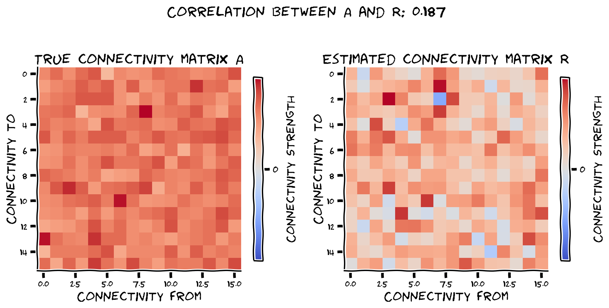
しかし、システムが複雑になると、相関は因果を捉えられなくなります。

セクション2.1: 複雑なシステムにおける相関の失敗

より大きなシステムに移りましょう。6ニューロンではなく、今回は100ニューロンを使います。結合行列の推定精度はどう変わるでしょうか？

# @markdown Execute this cell to simulate large system, estimate connectivity matrix with correlation and return estimation quality

# Simulate a 100 neuron system for 5000 timesteps.
n_neurons = 100
timesteps = 5000
random_state = 42

A = create_connectivity(n_neurons, random_state)
X = simulate_neurons(A, timesteps)
R = correlation_for_all_neurons(X)
corr = np.corrcoef(A.flatten(), R.flatten())[0, 1]

fig, axs = plt.subplots(1, 2, figsize=(12, 6))
plot_connectivity_matrix(A, ax=axs[0])
axs[0].set_title("True connectivity matrix A")
plot_connectivity_matrix(R, ax=axs[1])
axs[1].set_title("Estimated connectivity matrix R")
fig.suptitle(f"Correlation of A and R: {corr:.5f}")
fig.tight_layout()
plt.show()

# @title Video 3: Correlation vs causation in large systems
from ipywidgets import widgets
from IPython.display import YouTubeVideo
from IPython.display import IFrame
from IPython.display import display


class PlayVideo(IFrame):
  def __init__(self, id, source, page=1, width=400, height=300, **kwargs):
    self.id = id
    if source == 'Bilibili':
      src = f'https://player.bilibili.com/player.html?bvid={id}&page={page}'
    elif source == 'Osf':
      src = f'https://mfr.ca-1.osf.io/render?url=https://osf.io/download/{id}/?direct%26mode=render'
    super(PlayVideo, self).__init__(src, width, height, **kwargs)


def display_videos(video_ids, W=400, H=300, fs=1):
  tab_contents = []
  for i, video_id in enumerate(video_ids):
    out = widgets.Output()
    with out:
      if video_ids[i][0] == 'Youtube':
        video = YouTubeVideo(id=video_ids[i][1], width=W,
                             height=H, fs=fs, rel=0)
        print(f'Video available at https://youtube.com/watch?v={video.id}')
      else:
        video = PlayVideo(id=video_ids[i][1], source=video_ids[i][0], width=W,
                          height=H, fs=fs, autoplay=False)
        if video_ids[i][0] == 'Bilibili':
          print(f'Video available at https://www.bilibili.com/video/{video.id}')
        elif video_ids[i][0] == 'Osf':
          print(f'Video available at https://osf.io/{video.id}')
      display(video)
    tab_contents.append(out)
  return tab_contents


video_ids = [('Youtube', 'U4sV-7g8T08'), ('Bilibili', 'BV1uC4y1b76C')]
tab_contents = display_videos(video_ids, W=854, H=480)
tabs = widgets.Tab()
tabs.children = tab_contents
for i in range(len(tab_contents)):
  tabs.set_title(i, video_ids[i][0])
display(tabs)

# @title Submit your feedback
content_review(f"{feedback_prefix}_Correlation_causation_in_large_systems_Video")

セクション2.2: ネットワークサイズに対する相関

インタラクティブデモ 2.2.1: ニューロン数に対する結合推定

少数（6個）や多数（100個）のニューロンだけでなく、ニューロン数を系統的に変化させ、真の結合行列と推定行列の相関係数の変化をプロットします。

# @markdown Execute this cell to enable the widget
@widgets.interact(n_neurons=(6, 42, 3))
def plot_corrs(n_neurons=6):
  fig, axs = plt.subplots(1, 2, figsize=(10, 5))
  timesteps = 2000
  random_state = 42
  A = create_connectivity(n_neurons, random_state)
  X = simulate_neurons(A, timesteps)
  R = correlation_for_all_neurons(X)
  corr = np.corrcoef(A.flatten(), R.flatten())[0, 1]
  plot_connectivity_matrix(A, ax=axs[0])
  plot_connectivity_matrix(R, ax=axs[1])
  axs[0].set_title("True connectivity matrix A")
  axs[1].set_title("Estimated connectivity matrix R")
  fig.suptitle(f"Correlation of A and R: {corr:.2f}")
  plt.show()

もちろん、 $A$ のランダム性によるばらつきがあります。複数回の試行で平均を取り、関係性を見つけましょう。

# @markdown Execute this cell to plot connectivity estimation as a function of network size

n_trials = 5
timesteps = 1000  # shorter timesteps for faster running time
number_of_neurons = [5, 10, 25, 50, 100]
plot_estimation_quality_vs_n_neurons(number_of_neurons)

# @title Submit your feedback
content_review(f"{feedback_prefix}_Connectivity_estimation_as_a_function_of_number_of_neurons_Interactive_Demo")

インタラクティブデモ 2.2.2: $A$ のスパース性に対する結合推定

相関が大規模システムでのみ失敗するのは、 $A$ の種類によるのでは？と疑問に思うかもしれません。このデモでは、 $A$ のスパース性を変化させて結合推定を調べます。スパース性が低いほど推定は良くなるでしょうか、それとも悪くなるでしょうか？

# @markdown Execute this cell to enable the widget
@widgets.interact(sparsity=(0.01, 0.99, .01))
def plot_corrs(sparsity=0.9):
  fig, axs = plt.subplots(1, 2, figsize=(10, 5))
  timesteps = 2000
  random_state = 42
  n_neurons = 25
  A = create_connectivity(n_neurons, random_state, sparsity)
  X = simulate_neurons(A, timesteps)
  R = correlation_for_all_neurons(X)
  corr = np.corrcoef(A.flatten(), R.flatten())[0, 1]
  plot_connectivity_matrix(A, ax=axs[0])
  plot_connectivity_matrix(R, ax=axs[1])
  axs[0].set_title("True connectivity matrix A")
  axs[1].set_title("Estimated connectivity matrix R")
  fig.suptitle(f"Correlation of A and R: {corr:.2f}")
  plt.show()

# @title Submit your feedback
content_review(f"{feedback_prefix}_Connectivity_estimation_as_a_function_of_the_sparsity_A_Interactive_Demo")

セクション3: 因果性を振り返る

チュートリアル開始からここまでの推定所要時間: 34分

考えよう！3: 因果性を振り返る

以下の質問について、グループで約10分間話し合ってください。

あなたが書いた研究論文を思い出してください。以前の因果知識（例: メカニズム）を使っていましたか？それとも因果的な問いを立てていましたか？その因果関係を介入の言葉で表現してみてください。（「もし $A$ を $A'$ に強制したら、 $B$ は...」）
あなたの神経科学分野での介入手法にはどんなものがありますか？
以下の一般的な「つなぎ言葉」は介入的定義の因果関係を示唆していますか？（調節する、媒介する、生成する、変調する、形作る、基礎となる、生み出す、符号化する、誘導する、可能にする、保証する、支持する、促進する、決定する）
脳の次元数を（大まかに）どのくらいと推定しますか？ニューロン間の相関から結合を推定できると思いますか？なぜですか？

# @title Submit your feedback
content_review(f"{feedback_prefix}_Reflecting_on_causality_Discussion")

まとめ

チュートリアルの推定所要時間: 45分

# @title Video 4: Summary
from ipywidgets import widgets
from IPython.display import YouTubeVideo
from IPython.display import IFrame
from IPython.display import display


class PlayVideo(IFrame):
  def __init__(self, id, source, page=1, width=400, height=300, **kwargs):
    self.id = id
    if source == 'Bilibili':
      src = f'https://player.bilibili.com/player.html?bvid={id}&page={page}'
    elif source == 'Osf':
      src = f'https://mfr.ca-1.osf.io/render?url=https://osf.io/download/{id}/?direct%26mode=render'
    super(PlayVideo, self).__init__(src, width, height, **kwargs)


def display_videos(video_ids, W=400, H=300, fs=1):
  tab_contents = []
  for i, video_id in enumerate(video_ids):
    out = widgets.Output()
    with out:
      if video_ids[i][0] == 'Youtube':
        video = YouTubeVideo(id=video_ids[i][1], width=W,
                             height=H, fs=fs, rel=0)
        print(f'Video available at https://youtube.com/watch?v={video.id}')
      else:
        video = PlayVideo(id=video_ids[i][1], source=video_ids[i][0], width=W,
                          height=H, fs=fs, autoplay=False)
        if video_ids[i][0] == 'Bilibili':
          print(f'Video available at https://www.bilibili.com/video/{video.id}')
        elif video_ids[i][0] == 'Osf':
          print(f'Video available at https://osf.io/{video.id}')
      display(video)
    tab_contents.append(out)
  return tab_contents


video_ids = [('Youtube', 'hRyAN3yak_U'), ('Bilibili', 'BV1KK4y1x74w')]
tab_contents = display_videos(video_ids, W=854, H=480)
tabs = widgets.Tab()
tabs.children = tab_contents
for i in range(len(tab_contents)):
  tabs.set_title(i, video_ids[i][0])
display(tabs)

# @title Submit your feedback
content_review(f"{feedback_prefix}_Summary_Video")

まとめです。大規模システムでは相関 ≠ 因果であることはわかりました。しかし、大規模システムを粗くサンプリングした場合はどうでしょうか？グループ間の相関から、グループ間の有効な因果相互作用（重みの平均）を推定できるでしょうか？

上記のシミュレーションからは、グループあたりのニューロン数が増えても、グループ間の因果相互作用の推定精度が有意に向上する様子は見られませんでした。

すべてのチュートリアルを終えた後、もし興味があれば、以下のボーナスセクション1で相関を類似度指標として簡単に議論し、ボーナスセクション2で低解像度システムにおける因果性と相関について学んでください。

ボーナス

ボーナスセクション1: 類似度指標としての相関

ここで注意したいのは、すべてのチュートリアルで推定結合行列 $R$ と真の結合行列 $A$ の類似度を測るためにピアソン相関係数を使っていますが、 $A$ の要素は正規分布に従わず（実際は二値的）厳密にはピアソン相関の正しい使い方ではありません。

ピアソン相関はNumpyで簡単に計算でき、他の相関指標と定性的に似た結果を出すため使っています。類似度を計算する他の方法:

スピアマン順位相関（正規分布を仮定しない）
推定行列 $R$ を中央値で二値化し、コーエンのカッパなどの一致度解析を行う

もう一つ考慮すべきことは、 $A$ と $R$ の類似度を測りたいだけです。要素ごとの比較も一つの方法ですが、他に思いつく方法はありますか？行列の類似度はどうでしょうか？

ボーナスセクション2: 低解像度システム

神経科学でよくある状況は、大量のニューロン群の平均的な活動を観察することです（fMRI、EEG、LFPなどを想像してください）。この効果をシミュレートし、相関が群や領域の平均的な因果効果を復元できるかを問います。

類推の質についての注意: これは脳やfMRIの完全な類推ではありません。代わりに、*相関が因果を推定できない大規模システムで、少なくとも群間の平均的な結合を復元できるか？*を問いたいのです。

脳の違いに関する注意点:
結合はランダムと仮定していますが、実際の脳では平均化されるニューロンは入力・出力結合が相関しています。これにより、システムの真の次元が低くなるため、相関と因果の対応は平均効果で改善します。しかし、実際の脳はここで扱うより桁違いに大きく、実験者は完全に観察されたシステムを持ちません。

大規模システムのシミュレーション

次のセルを実行して、256ニューロンの大規模システムを10,000タイムステップでシミュレートします。完了まで少し時間がかかります（約4分）ので、実行中に先に進んでください。

# @markdown Execute this cell to simulate a large system

n_neurons = 256
timesteps = 10000
random_state = 42

A = create_connectivity(n_neurons, random_state)
X = simulate_neurons(A, timesteps)

ボーナスセクション1.1: システムを粗くサンプリングする

このシステムを直接観察するのではなく、グループの平均活動を観察します。

ボーナスコーディング演習1.1: グループごとの平均活動を計算し、得られた結合を真の結合と比較する

16グループの新しい行列 coarse_X を作成します。各グループは16ニューロンの平均活動を反映します（合計256ニューロンのため）。

次に、グループ間のニューロン結合強度の平均として真の粗結合行列を定義します。粗くサンプリングしたグループ間の相関から結合を推定し、真の結合と比較します。

def get_coarse_corr(n_groups, X):
  """
  A wrapper function for our correlation calculations between coarsely sampled
  A and R.

  Args:
    n_groups (int): the number of groups. should divide the number of neurons evenly
    X: the simulated system

  Returns:
    A single float correlation value representing the similarity between A and R
    ndarray: estimated connectivity matrix
    ndarray: true connectivity matrix
  """

  ############################################################################
  ## TODO: Insert your code here to get coarsely sampled X
  # Fill out function then remove
  raise NotImplementedError('Student exercise: please complete get_coarse_corr')
  ############################################################################
  coarse_X = ...

  # Make sure coarse_X is the right shape
  assert coarse_X.shape == (n_groups, timesteps)

  # Estimate connectivity from coarse system
  R = correlation_for_all_neurons(coarse_X)

  # Compute true coarse connectivity
  coarse_A = A.reshape(n_groups, n_neurons // n_groups, n_groups, n_neurons // n_groups).mean(3).mean(1)

  # Compute true vs estimated connectivity correlation
  corr = np.corrcoef(coarse_A.flatten(), R.flatten())[0, 1]

  return corr, R, coarse_A


n_groups = 16

# Call function
corr, R, coarse_A = get_coarse_corr(n_groups, X)

# Visualize
plot_true_vs_estimated_connectivity(R, coarse_A, correlation=corr)