「AがBを引き起こす」という文を慎重に考えてみましょう。具体的に2つのニューロンを例にとります。ニューロン$A$がニューロン$B$の発火を引き起こすとはどういう意味でしょうか？

介入的な因果性の定義は以下のように言います:

$A$が$B$の発火を引き起こすかどうかを判断するには、ニューロン$A$に電流を注入して$B$に何が起こるかを観察します。

因果性の数学的定義:
多くの試行の平均として、ニューロン$A$がニューロン$B$に及ぼす平均因果効果$\delta_{A\to B}$は、$A=1$に設定した場合と$A=0$に設定した場合の$B$の活動の平均変化です。

ここで$\mathbb{E}[B | A=1]$は$A$が1のときの$B$の期待値、$\mathbb{E}[B | A=0]$は$A$が0のときの$B$の期待値です。

これは平均効果であることに注意してください。条件付き効果（例えば$A$が不応期でないときのみ$B$に影響するなど）をより詳細に扱うこともできますが、今日は平均効果のみを考えます。

私たちのシステムはN個の相互接続されたニューロンからなり、時間を通じて互いに影響しあいます。各ニューロンの時刻$t+1$での状態は、前時刻$t$の他のニューロンの活動の関数です。

ニューロンは非線形に互いに影響します：各ニューロンの時刻$t+1$での活動は、時刻$t$のすべてのニューロン活動の線形加重和にノイズを加え、非線形関数を通したものです：

• $\vec{x}_t$は時刻$t$での$n$次元ベクトルで、$n$個のニューロンの状態を表します
• $\sigma$はシグモイド非線形関数
• $A$は$n \times n$の因果的真の接続行列（後述）
• $\epsilon_t$はランダムノイズで、$\epsilon_t \sim N(\vec{0}, I_n)$
• $\vec{x}_0$はゼロベクトルで初期化されます

$A$は接続行列で、要素$A_{ij}$はニューロン$i$がニューロン$j$に及ぼす因果効果を表します。システムでは、ニューロンは全体の約10%のニューロンから接続を受け取ります。

6つのニューロン間の真の接続行列を作成し、2つの異なる方法で可視化します：接続されたニューロン間の方向付きエッジを持つグラフとして、そして接続行列の画像として。

理解度チェック: 左のプロットが右のプロットにどう対応しているか理解できますか？

# @markdown Execute this cell to get helper function `create_connectivity` and visualize connectivity

def create_connectivity(n_neurons, random_state=42):
  """
  Generate our nxn causal connectivity matrix.

  Args:
    n_neurons (int): the number of neurons in our system.
    random_state (int): random seed for reproducibility

  Returns:
    A (np.ndarray): our 0.1 sparse connectivity matrix
  """
  np.random.seed(random_state)
  A_0 = np.random.choice([0, 1], size=(n_neurons, n_neurons), p=[0.9, 0.1])

  # set the timescale of the dynamical system to about 100 steps
  _, s_vals, _ = np.linalg.svd(A_0)
  A = A_0 / (1.01 * s_vals[0])

  # _, s_val_test, _ = np.linalg.svd(A)
  # assert s_val_test[0] < 1, "largest singular value >= 1"

  return A


# Initializes the system
n_neurons = 6
A = create_connectivity(n_neurons)

# Let's plot it!
plot_connectivity_graph_matrix(A)

コーディング演習2: システムのシミュレーション

この演習ではシステムをシミュレートします。以下の関数を完成させて、各時刻で活動ベクトル$x$が以下のように更新されるようにしてください:

補助関数sigmoidは以下のセルで定義されています。

# @markdown Execute to enable helper function `sigmoid`

def sigmoid(x):
  """
  Compute sigmoid nonlinearity element-wise on x

  Args:
      x (np.ndarray): the numpy data array we want to transform
  Returns
      (np.ndarray): x with sigmoid nonlinearity applied
  """
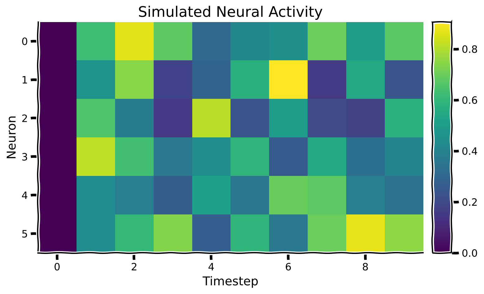
  return 1 / (1 + np.exp(-x))

def simulate_neurons(A, timesteps, random_state=42):
  """Simulates a dynamical system for the specified number of neurons and timesteps.

  Args:
    A (np.array): the connectivity matrix
    timesteps (int): the number of timesteps to simulate our system.
    random_state (int): random seed for reproducibility

  Returns:
    - X has shape (n_neurons, timeteps). A schematic:
                ___t____t+1___
    neuron  0  |   0    1     |
              |   1    0     |
    neuron  i  |   0 -> 1     |
              |   0    0     |
              |___1____0_____|
  """
  np.random.seed(random_state)

  n_neurons = len(A)
  X = np.zeros((n_neurons, timesteps))

  for t in range(timesteps - 1):

    # Create noise vector
    epsilon = np.random.multivariate_normal(np.zeros(n_neurons), np.eye(n_neurons))

    ########################################################################
    ## TODO: Fill in the update rule for our dynamical system.
    ## Fill in function and remove
    raise NotImplementedError("Complete simulate_neurons")
    ########################################################################

    # Update activity vector for next step
    X[:, t + 1] = sigmoid(...)  # we are using helper function sigmoid

  return X


# Set simulation length
timesteps = 5000

# Simulate our dynamical system
X = simulate_neurons(A, timesteps)

# Visualize
plot_neural_activity(X)

解答を見る$

例の出力:

# @title Submit your feedback
content_review(f"{feedback_prefix}_System_simulation_Exercise")

セクション3: 摂動による接続性の回復

チュートリアル開始からここまでの推定所要時間: 22分

# @title Video 3: Perturbing systems
from ipywidgets import widgets
from IPython.display import YouTubeVideo
from IPython.display import IFrame
from IPython.display import display


class PlayVideo(IFrame):
  def __init__(self, id, source, page=1, width=400, height=300, **kwargs):
    self.id = id
    if source == 'Bilibili':
      src = f'https://player.bilibili.com/player.html?bvid={id}&page={page}'
    elif source == 'Osf':
      src = f'https://mfr.ca-1.osf.io/render?url=https://osf.io/download/{id}/?direct%26mode=render'
    super(PlayVideo, self).__init__(src, width, height, **kwargs)


def display_videos(video_ids, W=400, H=300, fs=1):
  tab_contents = []
  for i, video_id in enumerate(video_ids):
    out = widgets.Output()
    with out:
      if video_ids[i][0] == 'Youtube':
        video = YouTubeVideo(id=video_ids[i][1], width=W,
                             height=H, fs=fs, rel=0)
        print(f'Video available at https://youtube.com/watch?v={video.id}')
      else:
        video = PlayVideo(id=video_ids[i][1], source=video_ids[i][0], width=W,
                          height=H, fs=fs, autoplay=False)
        if video_ids[i][0] == 'Bilibili':
          print(f'Video available at https://www.bilibili.com/video/{video.id}')
        elif video_ids[i][0] == 'Osf':
          print(f'Video available at https://osf.io/{video.id}')
      display(video)
    tab_contents.append(out)
  return tab_contents


video_ids = [('Youtube', 'wOZunGtuqQE'), ('Bilibili', 'BV1Hv411q7Ka')]
tab_contents = display_videos(video_ids, W=854, H=480)
tabs = widgets.Tab()
tabs.children = tab_contents
for i in range(len(tab_contents)):
  tabs.set_title(i, video_ids[i][0])
display(tabs)

# @title Submit your feedback
content_review(f"{feedback_prefix}_Perturbing_systems_Video")

セクション3.1: ニューロン系におけるランダム摂動

各ニューロンが他のニューロンに及ぼす因果効果を得たいです。因果効果の真の値は接続行列$A$です。

以下を計算したいことを思い出してください:

システムの状態をランダムに0または1に設定し、1タイムステップ後の結果を観察することでこれを行います。これを$N$回繰り返すと、ニューロン$i$がニューロン$j$に及ぼす効果は:

これは単にニューロン$j$の活動の2つの条件における平均差です。

上記の式を計算しますが、交互のタイムステップで活動に介入していると想像してください。

補助関数simulate_neurons_perturbを使います。前の演習のsimulate_neurons関数とほぼ同じですが、各タイムステップで以下を追加しています:

if t % 2 == 0:
    X[:,t] = np.random.choice([0,1], size=n_neurons)

これは交互のタイムステップで全ニューロンの活動が0か1にランダムに変更されることを意味します。

かなり強い摂動ですね。脳内でこんなことが起きてほしくないでしょう。

動的変化を視覚的に比較してみましょう: 次のセルを実行して、動的がどう変わったか見てみてください。

# @markdown Execute this cell to visualize perturbed dynamics
def simulate_neurons_perturb(A, timesteps):
  """
  Simulates a dynamical system for the specified number of neurons and timesteps,
  BUT every other timestep the activity is clamped to a random pattern of 1s and 0s

  Args:
    A (np.array): the true connectivity matrix
    timesteps (int): the number of timesteps to simulate our system.

  Returns:
    The results of the simulated system.
    - X has shape (n_neurons, timeteps)
  """
  n_neurons = len(A)
  X = np.zeros((n_neurons, timesteps))
  for t in range(timesteps - 1):
    if t % 2 == 0:
      X[:, t] = np.random.choice([0, 1], size=n_neurons)
    epsilon = np.random.multivariate_normal(np.zeros(n_neurons), np.eye(n_neurons))
    X[:, t + 1] = sigmoid(A.dot(X[:, t]) + epsilon)  # we are using helper function sigmoid

  return X


timesteps = 5000  # Simulate for 5000 timesteps.

# Simulate our dynamical system for the given amount of time
X_perturbed = simulate_neurons_perturb(A, timesteps)

# Plot our standard versus perturbed dynamics
fig, axs = plt.subplots(1, 2, figsize=(15, 4))
im0 = axs[0].imshow(X[:, :10])
im1 = axs[1].imshow(X_perturbed[:, :10])

# Matplotlib boilerplate code
divider = make_axes_locatable(axs[0])
cax0 = divider.append_axes("right", size="5%", pad=0.15)
plt.colorbar(im0, cax=cax0)

divider = make_axes_locatable(axs[1])
cax1 = divider.append_axes("right", size="5%", pad=0.15)
plt.colorbar(im1, cax=cax1)

axs[0].set_ylabel("Neuron", fontsize=15)
axs[1].set_xlabel("Timestep", fontsize=15)
axs[0].set_xlabel("Timestep", fontsize=15);
axs[0].set_title("Standard dynamics", fontsize=15)
axs[1].set_title("Perturbed dynamics", fontsize=15)
plt.show()

セクション3.2: 摂動された動的から接続性を回復する

# @title Video 4: Calculating causality
from ipywidgets import widgets
from IPython.display import YouTubeVideo
from IPython.display import IFrame
from IPython.display import display


class PlayVideo(IFrame):
  def __init__(self, id, source, page=1, width=400, height=300, **kwargs):
    self.id = id
    if source == 'Bilibili':
      src = f'https://player.bilibili.com/player.html?bvid={id}&page={page}'
    elif source == 'Osf':
      src = f'https://mfr.ca-1.osf.io/render?url=https://osf.io/download/{id}/?direct%26mode=render'
    super(PlayVideo, self).__init__(src, width, height, **kwargs)


def display_videos(video_ids, W=400, H=300, fs=1):
  tab_contents = []
  for i, video_id in enumerate(video_ids):
    out = widgets.Output()
    with out:
      if video_ids[i][0] == 'Youtube':
        video = YouTubeVideo(id=video_ids[i][1], width=W,
                             height=H, fs=fs, rel=0)
        print(f'Video available at https://youtube.com/watch?v={video.id}')
      else:
        video = PlayVideo(id=video_ids[i][1], source=video_ids[i][0], width=W,
                          height=H, fs=fs, autoplay=False)
        if video_ids[i][0] == 'Bilibili':
          print(f'Video available at https://www.bilibili.com/video/{video.id}')
        elif video_ids[i][0] == 'Osf':
          print(f'Video available at https://osf.io/{video.id}')
      display(video)
    tab_contents.append(out)
  return tab_contents


video_ids = [('Youtube', 'EDZtcsIAVGM'), ('Bilibili', 'BV15A411v7JS')]
tab_contents = display_videos(video_ids, W=854, H=480)
tabs = widgets.Tab()
tabs.children = tab_contents
for i in range(len(tab_contents)):
  tabs.set_title(i, video_ids[i][0])
display(tabs)

# @title Submit your feedback
content_review(f"{feedback_prefix}_Calculating_causality_Video")

コーディング演習3.2: 摂動された動的から接続性を回復する

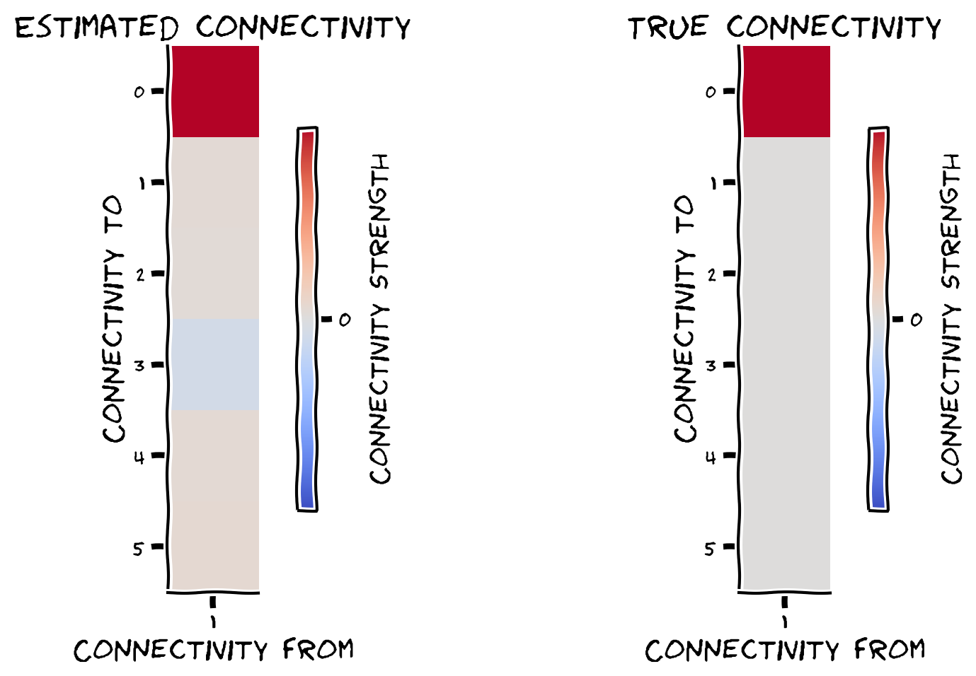
上記の摂動された動的から、システム内の単一のニューロン(selected_neuron)が他のすべてのニューロンに及ぼす因果効果を回復する関数を書いてください。上記の式を計算します:

交互のタイムステップで全ニューロンを摂動しましたが、この演習では単一のニューロンの因果効果の計算に集中します。$x^j_{t+1}$には摂動していないタイムステップ、$x^j_t$には摂動しているタイムステップを使います。numpyのインデックス指定はarray[開始:終了:間隔]で、例えば交互の要素を取得するにはarray[::2]とします。

def get_perturbed_connectivity_from_single_neuron(perturbed_X, selected_neuron):
  """
  Computes the connectivity matrix from the selected neuron using differences in means.

  Args:
    perturbed_X (np.ndarray): the perturbed dynamical system matrix of shape
                              (n_neurons, timesteps)
    selected_neuron (int): the index of the neuron we want to estimate connectivity for

  Returns:
      estimated_connectivity (np.ndarray): estimated connectivity for the selected neuron,
                                           of shape (n_neurons,)
  """
  # Extract the perturbations of neuron 1 (every other timestep)
  neuron_perturbations = perturbed_X[selected_neuron, ::2]

  # Extract the observed outcomes of all the neurons (every other timestep)
  all_neuron_output = perturbed_X[:, 1::2]

  # Initialize estimated connectivity matrix
  estimated_connectivity = np.zeros(n_neurons)

  # Loop over neurons
  for neuron_idx in range(n_neurons):

    # Get this output neurons (neuron_idx) activity
    this_neuron_output = all_neuron_output[neuron_idx, :]

    # Get timesteps where the selected neuron == 0 vs == 1
    one_idx = np.argwhere(neuron_perturbations == 1)
    zero_idx = np.argwhere(neuron_perturbations == 0)

    ########################################################################
    ## TODO: Insert your code here to compute the neuron activation from perturbations.
    # Fill out function and remove
    raise NotImplementedError("Complete the function get_perturbed_connectivity_single_neuron")
    ########################################################################

    difference_in_means = ...

    estimated_connectivity[neuron_idx] = difference_in_means

  return estimated_connectivity


# Initialize the system
n_neurons = 6
timesteps = 5000
selected_neuron = 1

# Simulate our perturbed dynamical system
perturbed_X = simulate_neurons_perturb(A, timesteps)

# Measure connectivity of neuron 1
estimated_connectivity = get_perturbed_connectivity_from_single_neuron(perturbed_X, selected_neuron)
plot_true_vs_estimated_connectivity(estimated_connectivity, A, selected_neuron)

解答を見る$

例の出力:

# @title Submit your feedback
content_review(f"{feedback_prefix}_Perturbed_dynamics_to_recover_connectivity_Exercise")

推定した接続行列と真の接続行列の類似度を相関係数で定量化できます。推定値と真の接続性の間にほぼ完全な相関が見られるはずです。そうなっていますか？

# Correlate true vs estimated connectivity matrix
print(np.corrcoef(A[:, selected_neuron], estimated_connectivity)[1, 0])

$A$の解釈についての注意: 厳密には$A$は因果効果の行列ではなく動的行列です。ではなぜ比較するのか？$A$と効果行列はどちらも有向接続がある場所以外は0であるため、効果を正しく推定できれば相関は1になるはずです。（ただしスケールは異なります。これは非線形関数$\sigma$が$x$の値を$[0,1]$に圧縮するためです。）チュートリアル2の付録で相関を指標として使うことについてさらに議論しています。

よくできました！単一ニューロンの接続性を推定できました。

次に同じ戦略を全ニューロンに対して使います。補助関数get_perturbed_connectivity_all_neuronsを用意しています。仕組みに興味があれば余裕があるときにボーナスセクション1を見てください。

# @markdown Execute to get helper function `get_perturbed_connectivity_all_neurons`

def get_perturbed_connectivity_all_neurons(perturbed_X):
  """
  Estimates the connectivity matrix of perturbations through stacked correlations.

  Args:
    perturbed_X (np.ndarray): the simulated dynamical system X of shape
                              (n_neurons, timesteps)

  Returns:
    R (np.ndarray): the estimated connectivity matrix of shape
                    (n_neurons, n_neurons)
  """
  # select perturbations (P) and outcomes (Outs)
  # we perturb the system every over time step, hence the 2 in slice notation
  P = perturbed_X[:, ::2]
  Outs = perturbed_X[:, 1::2]

  # stack perturbations and outcomes into a 2n by (timesteps / 2) matrix
  S = np.concatenate([P, Outs], axis=0)

  # select the perturbation -> outcome block of correlation matrix (upper right)
  R = np.corrcoef(S)[:n_neurons, n_neurons:]

  return R


# Parameters
n_neurons = 6
timesteps = 5000

# Generate nxn causal connectivity matrix
A = create_connectivity(n_neurons)

# Simulate perturbed dynamical system
perturbed_X = simulate_neurons_perturb(A, timesteps)

# Get estimated connectivity matrix
R = get_perturbed_connectivity_all_neurons(perturbed_X)

#@markdown Execute this cell to visualize true vs estimated connectivity

# Let's visualize the true connectivity and estimated connectivity together
fig, axs = plt.subplots(2, 2, figsize=(10, 10))
see_neurons(A, axs[0, 0])  # we are invoking a helper function that visualizes the connectivity matrix
plot_connectivity_matrix(A, ax=axs[0, 1])
axs[0, 1].set_title("True connectivity matrix A")

see_neurons(R.T, axs[1, 0])  # we are invoking a helper function that visualizes the connectivity matrix
plot_connectivity_matrix(R.T, ax=axs[1, 1])
axs[1, 1].set_title("Estimated connectivity matrix R")

fig.suptitle("True vs estimated connectivity")
plt.show()

再び真の接続行列と推定接続行列の要素間の相関係数を計算します。ほぼ1なので真の因果関係をよく回復できています！

print(np.corrcoef(A.transpose().flatten(), R.flatten())[1, 0])

まとめ

チュートリアルの推定所要時間: 40分

# @title Video 5: Summary
from ipywidgets import widgets
from IPython.display import YouTubeVideo
from IPython.display import IFrame
from IPython.display import display


class PlayVideo(IFrame):
  def __init__(self, id, source, page=1, width=400, height=300, **kwargs):
    self.id = id
    if source == 'Bilibili':
      src = f'https://player.bilibili.com/player.html?bvid={id}&page={page}'
    elif source == 'Osf':
      src = f'https://mfr.ca-1.osf.io/render?url=https://osf.io/download/{id}/?direct%26mode=render'
    super(PlayVideo, self).__init__(src, width, height, **kwargs)


def display_videos(video_ids, W=400, H=300, fs=1):
  tab_contents = []
  for i, video_id in enumerate(video_ids):
    out = widgets.Output()
    with out:
      if video_ids[i][0] == 'Youtube':
        video = YouTubeVideo(id=video_ids[i][1], width=W,
                             height=H, fs=fs, rel=0)
        print(f'Video available at https://youtube.com/watch?v={video.id}')
      else:
        video = PlayVideo(id=video_ids[i][1], source=video_ids[i][0], width=W,
                          height=H, fs=fs, autoplay=False)
        if video_ids[i][0] == 'Bilibili':
          print(f'Video available at https://www.bilibili.com/video/{video.id}')
        elif video_ids[i][0] == 'Osf':
          print(f'Video available at https://osf.io/{video.id}')
      display(video)
    tab_contents.append(out)
  return tab_contents


video_ids = [('Youtube', 'p3fZW5Woqa4'), ('Bilibili', 'BV1FT4y1j7PW')]
tab_contents = display_videos(video_ids, W=854, H=480)
tabs = widgets.Tab()
tabs.children = tab_contents
for i in range(len(tab_contents)):
  tabs.set_title(i, video_ids[i][0])
display(tabs)

# @title Submit your feedback
content_review(f"{feedback_prefix}_Summary_Video")

このチュートリアルでは、摂動を用いた因果性の定義と推定方法について学びました。特に以下を行いました:

1. 連結されたニューロン系のシミュレーション方法を学んだ

2. 神経活動を直接摂動することでニューロン間の接続性を推定する方法を学んだ

NMA終了後に因果性に興味がある方のために、参考になる文献を紹介します。

• ImbensとRubinによる『Causal Inference for Statistics, Social, and Biomedical Sciences』
• HernanとRubinによる『Causal Inference: What If』
• AngristとPischkeによる『Mostly Harmless Econometrics』
• 神経科学への応用例はこちらを参照してください

ボーナス

ボーナスセクション1: 推定接続行列の計算

これは$get_perturbed_connectivity_all_neurons()$のコードが何をしているかの説明です

まず推定接続行列$R$を計算します。摂動行列$P$と結果行列$O$を抽出します:

そして$P$と$O$を縦に連結した行列$S$の相関行列を計算します:

$R$は$\text{corr}(S)$の右上の$n \times n$ブロックとして抽出されます:

これは上部右ブロックがシステム内の各ニューロンペアに対する摂動の結果への効果を表すためです。

この方法は平均差分で得られる結果に比例する推定接続行列を与え、$x$の分散に依存する比例定数の違いのみがあります。