チュートリアル 4: モデルベース強化学習

第3週4日目: 強化学習

Neuromatch Academy 提供

コンテンツ制作者: Marcelo G Mattar, Eric DeWitt, Matt Krause, Matthew Sargent, Anoop Kulkarni, Sowmya Parthiban, Feryal Behbahani, Jane Wang

コンテンツレビュアー: Ella Batty, Byron Galbraith, Michael Waskom, Ezekiel Williams, Mehul Rastogi, Lily Cheng, Roberto Guidotti, Arush Tagade, Kelson Shilling-Scrivo

制作編集者: Gagana B, Spiros Chavlis

チュートリアルの目的

推定所要時間: 45分

このチュートリアルでは、報酬だけでなく、エージェントの行動が将来の状態にどのように影響するかを予測することを学習する、より複雑なエージェントをモデル化します。この追加情報により、エージェントは「計画」を用いて行動を選択できます。

最も単純なモデルベース強化学習アルゴリズムの一つであるDyna-Qを実装します。ワールドモデルとは何か、それがエージェントの方策をどのように改善するか、そしてモデルベースのアルゴリズムがモデルフリーのものより有利になる状況を理解します。

• 簡単なタスクを解くモデルベースRLエージェントDyna-Qを実装します;
• 計画がエージェントの行動に与える影響を調査します;
• 環境変化に対するモデルベースとモデルフリーエージェントの行動を比較します。

# @title Tutorial slides
# @markdown These are the slides for all videos in this tutorial.
from IPython.display import IFrame
link_id = "2jzdu"
print(f"If you want to download the slides: https://osf.io/download/{link_id}/")
IFrame(src=f"https://mfr.ca-1.osf.io/render?url=https://osf.io/{link_id}/?direct%26mode=render%26action=download%26mode=render", width=854, height=480)

セットアップ

# @title Install and import feedback gadget


from vibecheck import DatatopsContentReviewContainer
def content_review(notebook_section: str):
    return DatatopsContentReviewContainer(
        "",  # No text prompt
        notebook_section,
        {
            "url": "https://pmyvdlilci.execute-api.us-east-1.amazonaws.com/klab",
            "name": "neuromatch_cn",
            "user_key": "y1x3mpx5",
        },
    ).render()


feedback_prefix = "W3D4_T4"

# Imports
import numpy as np
import matplotlib.pyplot as plt
from scipy.signal import convolve as conv

# @title Figure Settings
import logging
logging.getLogger('matplotlib.font_manager').disabled = True
%config InlineBackend.figure_format = 'retina'
plt.style.use("https://raw.githubusercontent.com/NeuromatchAcademy/course-content/main/nma.mplstyle")

#@title Plotting Functions

def plot_state_action_values(env, value, ax=None):
  """
  Generate plot showing value of each action at each state.
  """
  if ax is None:
    fig, ax = plt.subplots()

  for a in range(env.n_actions):
    ax.plot(range(env.n_states), value[:, a], marker='o', linestyle='--')
  ax.set(xlabel='States', ylabel='Values')
  ax.legend(['R','U','L','D'], loc='lower right')


def plot_quiver_max_action(env, value, ax=None):
  """
  Generate plot showing action of maximum value or maximum probability at
    each state (not for n-armed bandit or cheese_world).
  """
  if ax is None:
    fig, ax = plt.subplots()

  X = np.tile(np.arange(env.dim_x), [env.dim_y,1]) + 0.5
  Y = np.tile(np.arange(env.dim_y)[::-1][:,np.newaxis], [1,env.dim_x]) + 0.5
  which_max = np.reshape(value.argmax(axis=1), (env.dim_y,env.dim_x))
  which_max = which_max[::-1,:]
  U = np.zeros(X.shape)
  V = np.zeros(X.shape)
  U[which_max == 0] = 1
  V[which_max == 1] = 1
  U[which_max == 2] = -1
  V[which_max == 3] = -1

  ax.quiver(X, Y, U, V)
  ax.set(
      title='Maximum value/probability actions',
      xlim=[-0.5, env.dim_x+0.5],
      ylim=[-0.5, env.dim_y+0.5],
  )
  ax.set_xticks(np.linspace(0.5, env.dim_x-0.5, num=env.dim_x))
  ax.set_xticklabels(["%d" % x for x in np.arange(env.dim_x)])
  ax.set_xticks(np.arange(env.dim_x+1), minor=True)
  ax.set_yticks(np.linspace(0.5, env.dim_y-0.5, num=env.dim_y))
  ax.set_yticklabels(["%d" % y for y in np.arange(0, env.dim_y*env.dim_x, env.dim_x)])
  ax.set_yticks(np.arange(env.dim_y+1), minor=True)
  ax.grid(which='minor',linestyle='-')


def plot_heatmap_max_val(env, value, ax=None):
  """
  Generate heatmap showing maximum value at each state
  """
  if ax is None:
    fig, ax = plt.subplots()

  if value.ndim == 1:
      value_max = np.reshape(value, (env.dim_y,env.dim_x))
  else:
      value_max = np.reshape(value.max(axis=1), (env.dim_y,env.dim_x))
  value_max = value_max[::-1,:]

  im = ax.imshow(value_max, aspect='auto', interpolation='none', cmap='afmhot')
  ax.set(title='Maximum value per state')
  ax.set_xticks(np.linspace(0, env.dim_x-1, num=env.dim_x))
  ax.set_xticklabels(["%d" % x for x in np.arange(env.dim_x)])
  ax.set_yticks(np.linspace(0, env.dim_y-1, num=env.dim_y))
  if env.name != 'windy_cliff_grid':
      ax.set_yticklabels(
          ["%d" % y for y in np.arange(
              0, env.dim_y*env.dim_x, env.dim_x)][::-1])
  return im


def plot_rewards(n_episodes, rewards, average_range=10, ax=None):
  """
  Generate plot showing total reward accumulated in each episode.
  """
  if ax is None:
    fig, ax = plt.subplots()

  smoothed_rewards = (conv(rewards, np.ones(average_range), mode='same')
                      / average_range)

  ax.plot(range(0, n_episodes, average_range),
          smoothed_rewards[0:n_episodes:average_range],
          marker='o', linestyle='--')
  ax.set(xlabel='Episodes', ylabel='Total reward')


def plot_performance(env, value, reward_sums):
  fig, axes = plt.subplots(nrows=2, ncols=2, figsize=(16, 12))
  plot_state_action_values(env, value, ax=axes[0,0])
  plot_quiver_max_action(env, value, ax=axes[0,1])
  plot_rewards(n_episodes, reward_sums, ax=axes[1,0])
  im = plot_heatmap_max_val(env, value, ax=axes[1,1])
  fig.colorbar(im)

#@title Helper Functions
def epsilon_greedy(q, epsilon):
  """Epsilon-greedy policy: selects the maximum value action with probability
  (1-epsilon) and selects randomly with epsilon probability.

  Args:
    q (ndarray): an array of action values
    epsilon (float): probability of selecting an action randomly

  Returns:
    int: the chosen action
  """
  be_greedy = np.random.random() > epsilon
  if be_greedy:
    action = np.argmax(q)
  else:
    action = np.random.choice(len(q))

  return action


def q_learning(state, action, reward, next_state, value, params):
  """Q-learning: updates the value function and returns it.

  Args:
    state (int): the current state identifier
    action (int): the action taken
    reward (float): the reward received
    next_state (int): the transitioned to state identifier
    value (ndarray): current value function of shape (n_states, n_actions)
    params (dict): a dictionary containing the default parameters

  Returns:
    ndarray: the updated value function of shape (n_states, n_actions)
  """
  # value of previous state-action pair
  prev_value = value[int(state), int(action)]

  # maximum Q-value at current state
  if next_state is None or np.isnan(next_state):
      max_value = 0
  else:
      max_value = np.max(value[int(next_state)])

  # reward prediction error
  delta = reward + params['gamma'] * max_value - prev_value

  # update value of previous state-action pair
  value[int(state), int(action)] = prev_value + params['alpha'] * delta

  return value


def learn_environment(env, model_updater, planner, params, max_steps,
                      n_episodes, shortcut_episode=None):
  # Start with a uniform value function
  value = np.ones((env.n_states, env.n_actions))

  # Run learning
  reward_sums = np.zeros(n_episodes)
  episode_steps = np.zeros(n_episodes)

  # Dyna-Q state
  model = np.nan*np.zeros((env.n_states, env.n_actions, 2))

  # Loop over episodes
  for episode in range(n_episodes):
    if shortcut_episode is not None and episode == shortcut_episode:
      env.toggle_shortcut()
      state = 64
      action = 1
      next_state, reward = env.get_outcome(state, action)
      model[state, action] = reward, next_state
      value = q_learning(state, action, reward, next_state, value, params)


    state = env.init_state  # initialize state
    reward_sum = 0

    for t in range(max_steps):
      # choose next action
      action = epsilon_greedy(value[state], params['epsilon'])

      # observe outcome of action on environment
      next_state, reward = env.get_outcome(state, action)

      # sum rewards obtained
      reward_sum += reward

      # update value function
      value = q_learning(state, action, reward, next_state, value, params)

      # update model
      model = model_updater(model, state, action, reward, next_state)

      # execute planner
      value = planner(model, value, params)

      if next_state is None:
        break  # episode ends
      state = next_state

    reward_sums[episode] = reward_sum
    episode_steps[episode] = t+1

  return value, reward_sums, episode_steps


class world(object):
    def __init__(self):
        return

    def get_outcome(self):
        print("Abstract method, not implemented")
        return

    def get_all_outcomes(self):
        outcomes = {}
        for state in range(self.n_states):
            for action in range(self.n_actions):
                next_state, reward = self.get_outcome(state, action)
                outcomes[state, action] = [(1, next_state, reward)]
        return outcomes

class QuentinsWorld(world):
    """
    World: Quentin's world.
    100 states (10-by-10 grid world).
    The mapping from state to the grid is as follows:
    90 ...       99
    ...
    40 ...       49
    30 ...       39
    20 21 22 ... 29
    10 11 12 ... 19
    0  1  2  ...  9
    54 is the start state.
    Actions 0, 1, 2, 3 correspond to right, up, left, down.
    Moving anywhere from state 99 (goal state) will end the session.
    Landing in red states incurs a reward of -1.
    Landing in the goal state (99) gets a reward of 1.
    Going towards the border when already at the border will stay in the same
        place.
    """
    def __init__(self):
        self.name = "QuentinsWorld"
        self.n_states = 100
        self.n_actions = 4
        self.dim_x = 10
        self.dim_y = 10
        self.init_state = 54
        self.shortcut_state = 64

    def toggle_shortcut(self):
      if self.shortcut_state == 64:
        self.shortcut_state = 2
      else:
        self.shortcut_state = 64

    def get_outcome(self, state, action):
        if state == 99:  # goal state
            reward = 0
            next_state = None
            return next_state, reward
        reward = 0  # default reward value
        if action == 0:  # move right
            next_state = state + 1
            if state == 98:  # next state is goal state
                reward = 1
            elif state % 10 == 9:  # right border
                next_state = state
            elif state in [11, 21, 31, 41, 51, 61, 71,
                           12, 72,
                           73,
                           14, 74,
                           15, 25, 35, 45, 55, 65, 75]:  # next state is red
                reward = -1
        elif action == 1:  # move up
            next_state = state + 10
            if state == 89:  # next state is goal state
                reward = 1
            if state >= 90:  # top border
                next_state = state
            elif state in [2, 12, 22, 32, 42, 52, 62,
                           3, 63,
                           self.shortcut_state,
                           5, 65,
                           6, 16, 26, 36, 46, 56, 66]:  # next state is red
                reward = -1
        elif action == 2:  # move left
            next_state = state - 1
            if state % 10 == 0:  # left border
                next_state = state
            elif state in [17, 27, 37, 47, 57, 67, 77,
                           16, 76,
                           75,
                           14, 74,
                           13, 23, 33, 43, 53, 63, 73]:  # next state is red
                reward = -1
        elif action == 3:  # move down
            next_state = state - 10
            if state <= 9:  # bottom border
                next_state = state
            elif state in [22, 32, 42, 52, 62, 72, 82,
                           23, 83,
                           84,
                           25, 85,
                           26, 36, 46, 56, 66, 76, 86]:  # next state is red
                reward = -1
        else:
            print("Action must be between 0 and 3.")
            next_state = None
            reward = None
        return int(next_state) if next_state is not None else None, reward

セクション1: モデルベースRL

# @title Video 1: Model-based RL
from ipywidgets import widgets
from IPython.display import YouTubeVideo
from IPython.display import IFrame
from IPython.display import display


class PlayVideo(IFrame):
  def __init__(self, id, source, page=1, width=400, height=300, **kwargs):
    self.id = id
    if source == 'Bilibili':
      src = f'https://player.bilibili.com/player.html?bvid={id}&page={page}'
    elif source == 'Osf':
      src = f'https://mfr.ca-1.osf.io/render?url=https://osf.io/download/{id}/?direct%26mode=render'
    super(PlayVideo, self).__init__(src, width, height, **kwargs)


def display_videos(video_ids, W=400, H=300, fs=1):
  tab_contents = []
  for i, video_id in enumerate(video_ids):
    out = widgets.Output()
    with out:
      if video_ids[i][0] == 'Youtube':
        video = YouTubeVideo(id=video_ids[i][1], width=W,
                             height=H, fs=fs, rel=0)
        print(f'Video available at https://youtube.com/watch?v={video.id}')
      else:
        video = PlayVideo(id=video_ids[i][1], source=video_ids[i][0], width=W,
                          height=H, fs=fs, autoplay=False)
        if video_ids[i][0] == 'Bilibili':
          print(f'Video available at https://www.bilibili.com/video/{video.id}')
        elif video_ids[i][0] == 'Osf':
          print(f'Video available at https://osf.io/{video.id}')
      display(video)
    tab_contents.append(out)
  return tab_contents


video_ids = [('Youtube', 'zT_legTotF0'), ('Bilibili', 'BV1Zv411i7gi')]
tab_contents = display_videos(video_ids, W=854, H=480)
tabs = widgets.Tab()
tabs.children = tab_contents
for i in range(len(tab_contents)):
  tabs.set_title(i, video_ids[i][0])
display(tabs)

# @title Submit your feedback
content_review(f"{feedback_prefix}_ModelBased_RL_Video")

前回のチュートリアルで紹介したアルゴリズムはすべてモデルフリーで、行動や制御にモデルを必要としませんでした。このセクションでは、モデルベースと呼ばれる別のクラスのアルゴリズムを学びます。次に見るように、モデルフリーRLとは対照的に、モデルベース手法はモデルを使って方策を構築します。

ではモデルとは何でしょうか？モデル（時にワールドモデルや内部モデルとも呼ばれます）は、エージェントの行動に対して世界がどのように反応するかの表現です。世界がどのように動くかの表現と考えることができます。このような表現を持つことで、エージェントは新しい経験をシミュレートし、それらのシミュレーションから学習できます。これは2つの理由で有利です。まず、現実世界で行動することはコストがかかり、時には危険なこともあります。チュートリアル3のクリフワールドを思い出してください。シミュレーション経験から学ぶことで、これらのコストやリスクを回避できます。次に、シミュレーションは限られた経験をより有効に活用します。なぜかというと、現実世界でエージェントが相互作用する場合、各行動で得られる情報はその瞬間にしか吸収できません。一方、モデルからシミュレートされた経験は何度でも、望むときにシミュレートできるため、情報をより完全に吸収できます。

クエンティンの世界環境

このチュートリアルでは、RLエージェントは10x10のグリッドワールド「クエンティンの世界」で行動します。

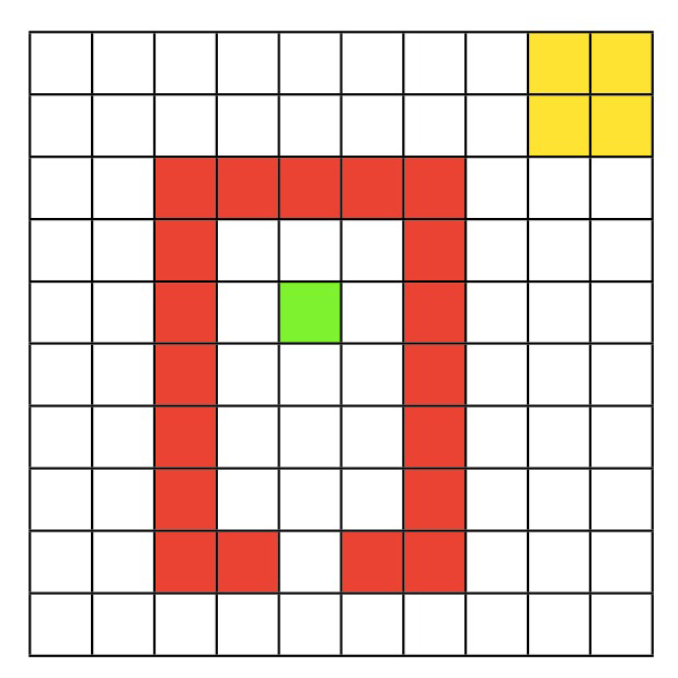
この環境には100の状態があり、4つの可能な行動（右、上、左、下）があります。エージェントの目標は、スタート地点（緑）からゴール領域（黄色）まで一連のステップで移動し、赤い壁を避けることです。具体的には：

• エージェントは緑の状態から開始します。
• 赤い状態に移動すると報酬は-1です。
• 世界の境界に移動しようとすると同じ場所に留まります。
• ゴール状態（右上の黄色のマス）に移動すると報酬は1です。
• ゴール状態からの移動はエピソードの終了を意味します。

環境とタスクが定義できたので、モデルベースRLエージェントでこれをどう解くか考えましょう。

セクション2: Dyna-Q

ここまでの推定所要時間: 11分

このセクションでは、最も単純なモデルベース強化学習アルゴリズムの一つ、Dyna-Qを実装します。Dyna-Qエージェントは行動、学習、計画を組み合わせます。最初の2つの要素、行動と学習はこれまで学んだものと同じです。例えばQ学習は、世界で行動しながら学習するため、行動と学習を組み合わせています。しかしDyna-Qエージェントは計画も実装し、モデルからの経験をシミュレートし、それから学習します。

理論的にはDyna-Qエージェントは行動、学習、計画を同時に常に実行していると考えられますが、実際にはアルゴリズムを一連のステップとして定義する必要があります。最も一般的な実装方法は、Q学習エージェントに計画ルーチンを追加することです。エージェントが実世界で行動し観察した経験から学習した後、$k$回の計画ステップを許可します。各計画ステップで、モデルは過去に経験した状態-行動ペアの履歴からランダムにサンプリングしてシミュレート経験を生成します。エージェントはこのシミュレート経験から、実際の経験から学習したのと同じQ学習ルールで学習します。このシミュレート経験は単一ステップの遷移、すなわち状態、行動、結果の状態と報酬です。つまり実際には、Dyna-Qエージェントは行動中の実際の経験1ステップから学習し、その後計画中に$k$ステップのシミュレート経験から学習します。

このアルゴリズムの最後の詳細は、シミュレート経験はどこから来るのか、つまり「モデル」とは何かです。Dyna-Qでは、エージェントが環境と相互作用するにつれてモデルも学習します。簡単のため、Dyna-Qはモデル学習をほぼ単純に、各遷移の結果をキャッシュする形で実装します。したがって、環境での各単一ステップ遷移の後、エージェントはこの遷移の結果を大きな行列に保存し、計画ステップごとにその行列を参照します。もちろん、このモデル学習戦略は世界が決定論的（各状態-行動ペアが常に同じ状態と報酬に遷移する）場合にのみ意味がありますが、以下の演習もこの設定です。しかし、この単純な設定でもDyna-Qの大きな強みの一つを示せます。すなわち、計画が環境との相互作用と同時に行われるため、相互作用から得られた新情報がモデルを変え、計画に興味深い影響を与える可能性があることです。

前回のチュートリアルでQ学習を実装済みなので、ここではDyna-Qに新たに加わるモデル更新ステップと計画ステップに焦点を当てます。参考までに、実装を手伝うDyna-Qアルゴリズムは以下の通りです。

表形式DYNA-Q

すべての$s \in S$と$a \in A$について$Q(s,a)$と$Model(s,a)$を初期化する。

無限ループ:

(a) $S$ ← 現在の（非終端）状態

(b) $A$ ← $\epsilon$-greedy$(S,Q)$

(c) 行動$A$を取り、報酬$R$と次状態$S'$を観察

(d) $Q(S,A)$ ← $Q(S,A) + \alpha \left[R + \gamma \max_{a} Q(S',a) - Q(S,A)\right]$

(e) $Model(S,A)$ ← $R,S'$ （決定論的環境を仮定）

(f) $k$回繰り返す:

$S$ ← 過去に観察した状態からランダムに選択

$A$ ← $S$で過去に取った行動からランダムに選択

$R,S'$ ← $Model(S,A)$

$Q(S,A)$ ← $Q(S,A) + \alpha \left[R + \gamma \max_{a} Q(S',a) - Q(S,A)\right]$

コーディング演習 2.1: Dyna-Q モデル更新

この演習ではDyna-Qアルゴリズムのモデル更新部分を実装します。具体的には、エージェントが環境で行動を実行した後、その状態-行動ペアに対して最後に経験した報酬と次状態を記憶するためにモデルを更新する必要があります。

def dyna_q_model_update(model, state, action, reward, next_state):
  """ Dyna-Q model update

  Args:
    model (ndarray): An array of shape (n_states, n_actions, 2) that represents
                     the model of the world i.e. what reward and next state do
                     we expect from taking an action in a state.
    state (int): the current state identifier
    action (int): the action taken
    reward (float): the reward received
    next_state (int): the transitioned to state identifier

  Returns:
    ndarray: the updated model
  """
  ###############################################################
  ## TODO for students: implement the model update step of Dyna-Q
  # Fill out function and remove
  raise NotImplementedError("Student exercise: implement the model update step of Dyna-Q")
  ###############################################################

  # Update our model with the observed reward and next state
  model[...] = ...

  return model

解答を見る$

# @title Submit your feedback
content_review(f"{feedback_prefix}_DynaQ_model_update_Exercise")

モデルを更新する方法ができたので、Dyna-Qの計画フェーズで過去の経験をシミュレートするために使えます。

コーディング演習 2.2: Dyna-Q 計画

この演習ではDyna-Qのもう一つの重要な部分、計画を実装します。経験した状態-行動ペアからランダムにサンプリングし、その状態でその行動を取った経験をモデルでシミュレートし、Q学習を使ってこれらのシミュレートされた状態、行動、報酬、次状態の結果から価値関数を更新します。さらに、この計画ステップを$k$回繰り返します。$k$はparams['k']から取得できます。

この演習では、Q学習の価値関数更新を処理するためにq_learning関数を使って構いません。メソッドのシグネチャはq_learning(state, action, reward, next_state, value, params)で、更新されたvalueテーブルを返します。

この関数を完成させると、モデルを更新する方法と計画に使う手段ができるので、実際に動かしてみます。コードはエージェントのパラメータと学習環境を設定し、あなたのモデル更新と計画メソッドを渡してクエンティンの世界を解かせます。計画ステップ数$k=10$に設定していることに注意してください。

def dyna_q_planning(model, value, params):
  """ Dyna-Q planning

  Args:
    model (ndarray): An array of shape (n_states, n_actions, 2) that represents
                     the model of the world i.e. what reward and next state do
                     we expect from taking an action in a state.
    value (ndarray): current value function of shape (n_states, n_actions)
    params (dict): a dictionary containing learning parameters

  Returns:
    ndarray: the updated value function of shape (n_states, n_actions)
  """
  ############################################################
  ## TODO for students: implement the planning step of Dyna-Q
  # Fill out function and remove
  raise NotImplementedError("Student exercise: implement the planning step of Dyna-Q")
  #############################################################
  # Perform k additional updates at random (planning)
  for _ in range(...):
    # Find state-action combinations for which we've experienced a reward i.e.
    # the reward value is not NaN. The outcome of this expression is an Nx2
    # matrix, where each row is a state and action value, respectively.
    candidates = np.array(np.where(~np.isnan(model[:,:,0]))).T

    # Write an expression for selecting a random row index from our candidates
    idx = ...

    # Obtain the randomly selected state and action values from the candidates
    state, action = ...

    # Obtain the expected reward and next state from the model
    reward, next_state = ...

    # Update the value function using Q-learning
    value = ...

  return value


# set for reproducibility, comment out / change seed value for different results
np.random.seed(1)

# parameters needed by our policy and learning rule
params = {
  'epsilon': 0.05,  # epsilon-greedy policy
  'alpha': 0.5,  # learning rate
  'gamma': 0.8,  # temporal discount factor
  'k': 10,  # number of Dyna-Q planning steps
}

# episodes/trials
n_episodes = 500
max_steps = 1000

# environment initialization
env = QuentinsWorld()

# solve Quentin's World using Dyna-Q
results = learn_environment(env, dyna_q_model_update, dyna_q_planning,
                            params, max_steps, n_episodes)
value, reward_sums, episode_steps = results

# Plot the results
plot_performance(env, value, reward_sums)

解答を見る$

出力例:

# @title Submit your feedback
content_review(f"{feedback_prefix}_DynaQ_planning_Exercise")

完了すると、Dyna-Qエージェントがタスクを非常に迅速に解決し、限られたエピソード数の後に安定して正の報酬を得ることができることがわかります（左下のグラフ）。

セクション3: どれだけ計画するか？

ここまでの推定所要時間: 30分

$k=10$のDyna-Qエージェントを実装したので、計画が性能に与える影響を理解しましょう。$k$の値を変えると学習能力にどのような影響があるでしょうか？

以下のコードは先ほどのコードに似ていますが、複数の$k$の値で複数回実験を行い、平均性能を比較します。特に$k \in \{0, 1, 10, 100\}$を選びます。$k=0$は計画なし、つまり通常のQ学習に相当することに注目してください。

このコードは完了までに少し時間がかかります。高速化したい場合は、実験回数や比較する$k$の値を減らしてみてください。

# set for reproducibility, comment out / change seed value for different results
np.random.seed(1)

# parameters needed by our policy and learning rule
params = {
  'epsilon': 0.05,  # epsilon-greedy policy
  'alpha': 0.5,  # learning rate
  'gamma': 0.8,  # temporal discount factor
}

# episodes/trials
n_experiments = 10
n_episodes = 100
max_steps = 1000

# number of planning steps
planning_steps = np.array([0, 1, 10, 100])

# environment initialization
env = QuentinsWorld()

steps_per_episode = np.zeros((len(planning_steps), n_experiments, n_episodes))

for i, k in enumerate(planning_steps):
  params['k'] = k
  for experiment in range(n_experiments):
    results = learn_environment(env, dyna_q_model_update, dyna_q_planning,
                                params, max_steps, n_episodes)
    steps_per_episode[i, experiment] = results[2]

# Average across experiments
steps_per_episode = np.mean(steps_per_episode, axis=1)

# Plot results
fig, ax = plt.subplots()
ax.plot(steps_per_episode.T)
ax.set(xlabel='Episodes', ylabel='Steps per episode',
       xlim=[20, None], ylim=[0, 160])
ax.legend(planning_steps, loc='upper right', title="Planning steps");

最初の20エピソードのウォームアップ期間の後、計画ステップ数がエージェントの環境を迅速に解決する能力に明確な影響を与えることがわかります。また、ある値を超えると相対的な効用が下がるため、学習を速めるのに十分な大きさの$k$を選びつつ、計画に無駄な時間をかけすぎないバランスが重要です。

セクション4: 世界が変わったら...

ここまでの推定所要時間: 37分

計画は新しい環境の学習を速めるだけでなく、環境の新情報を方策に素早く取り込むのにも役立ちます。つまり、環境が変わった場合（例えば状態間遷移のルールや状態/行動に関連する報酬）、エージェントはその変化を繰り返し実際に経験する必要はありません（Q学習エージェントなら必要です）。代わりに計画により、その変化を一度の経験で素早く方策に反映できます。

この最後のセクションでは再びエージェントにクエンティンの世界を解かせますが、200エピソード後に環境に近道が現れます。モデルフリーのQ学習エージェントと計画ステップを持つDyna-Qエージェントがこの環境変化にどう適応するかを比較します。

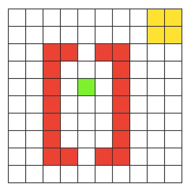
以下のコードもこれまでと似ています。複数の$k$の値を使い、$k=0$はQ学習エージェント、$k=10$は10回計画ステップを持つDyna-Qエージェントです。主な違いは近道が現れるタイミングを示すインジケーターを追加したことです。エージェントは400エピソード実行し、200エピソード目の途中で近道が現れます。

近道が現れた際、各エージェントはその変化を一度だけ経験します。具体的には、近道の下の状態で上方向に移動する行動を一度評価します。その後、エージェントは環境との相互作用を続けます。

# set for reproducibility, comment out / change seed value for different results
np.random.seed(1)

# parameters needed by our policy and learning rule
params = {
  'epsilon': 0.05,  # epsilon-greedy policy
  'alpha': 0.5,  # learning rate
  'gamma': 0.8,  # temporal discount factor
}

# episodes/trials
n_episodes = 400
max_steps = 1000
shortcut_episode = 200  # when we introduce the shortcut

# number of planning steps
planning_steps = np.array([0, 10]) # Q-learning, Dyna-Q (k=10)

# environment initialization
steps_per_episode = np.zeros((len(planning_steps), n_episodes))

# Solve Quentin's World using Q-learning and Dyna-Q
for i, k in enumerate(planning_steps):
  env = QuentinsWorld()
  params['k'] = k
  results = learn_environment(env, dyna_q_model_update, dyna_q_planning,
                              params, max_steps, n_episodes,
                              shortcut_episode=shortcut_episode)
  steps_per_episode[i] = results[2]


# Plot results
fig, ax = plt.subplots()
ax.plot(steps_per_episode.T)
ax.set(xlabel='Episode', ylabel='Steps per Episode',
       xlim=[20,None], ylim=[0, 160])
ax.axvline(shortcut_episode, linestyle="--", color='gray', label="Shortcut appears")
ax.legend(('Q-learning', 'Dyna-Q', 'Shortcut appears'),
          loc='upper right');

うまくいけば、Dyna-Qエージェントは近道が現れる前にほぼ最適な性能を達成し、その新情報を即座に取り込んでさらに改善します。一方、Q学習エージェントは新しい近道を完全に取り込むまでにずっと時間がかかります。

まとめ

推定所要時間: 45分

このノートブックではモデルベース強化学習について学び、その中でも最も単純なアーキテクチャの一つであるDyna-Qを実装しました。Dyna-QはQ学習に非常によく似ていますが、実際の経験だけでなくシミュレートされた経験からも学習します。この小さな違いが大きな利点をもたらします！計画はエージェントを環境の制約から解放し、その結果学習を加速します。例えば環境変化を効果的に方策に取り込むことができます。

当然ながら、モデルベースRLは機械学習の活発な研究分野です。最先端の興味深いテーマには、(i) 複雑なワールドモデルの学習と表現（上記の表形式かつ決定論的なケースを超えて）、(ii) 何をシミュレートするか（探索制御とも呼ばれ、上記のランダム選択を超えて）などがあります。

この枠組みは神経科学でも計画、記憶サンプリング、記憶の固定化、さらには夢の説明など様々な現象の解明に使われています。