チュートリアル 3: 行動を学ぶ：Qラーニング

第3週4日目：強化学習

Neuromatch Academyによる

コンテンツ作成者: Marcelo G Mattar, Eric DeWitt, Matt Krause, Matthew Sargent, Anoop Kulkarni, Sowmya Parthiban, Feryal Behbahani, Jane Wang

コンテンツレビュアー: Ella Batty, Byron Galbraith, Michael Waskom, Ezekiel Williams, Mehul Rastogi, Lily Cheng, Roberto Guidotti, Arush Tagade, Kelson Shilling-Scrivo

チュートリアルの目的

推定所要時間：40分

このチュートリアルでは、行動が即時に得られる報酬だけでなく（チュートリアル2のように）、世界の状態自体にも影響を与え、その結果将来の報酬の可能性にも影響を及ぼす、やや複雑な行動エージェントをモデル化します。したがって、これらのエージェントはチュートリアル1で学んだ将来の報酬の予測を活用し、即時の報酬と将来のより高い報酬の可能性とのトレードオフを理解する必要があります。

マルコフ決定過程（MDP）で形式化された、より現実的な連続的意思決定の設定で行動する方法を学びます。連続的意思決定問題では、ある状態で実行される行動は即時の報酬をもたらすだけでなく（バンディット問題のように）、次に経験する状態にも影響を与えます（バンディット問題とは異なります）。したがって、各行動は将来のすべての報酬に影響を与える可能性があります。このため、この設定での意思決定は、各行動の期待される累積将来報酬の観点から考慮する必要があります。

ここでは空間ナビゲーションの例を考えます。ある状態（位置）での行動（移動）が次に経験する状態に影響を与え、報酬を得るまでに一連の行動を実行する必要がある場合があります。

このチュートリアルの終わりまでに、以下を学びます。

グリッドワールドとは何か、そしてそれが単純な強化学習エージェントの評価にどのように役立つか
行動価値を推定するQラーニングアルゴリズムの基本
バンディット問題で復習した探索と活用の概念が、連続的意思決定の設定にもどのように適用されるか

# @title Tutorial slides
# @markdown These are the slides for all videos in this tutorial.
from IPython.display import IFrame
link_id = "2jzdu"
print(f"If you want to download the slides: https://osf.io/download/{link_id}/")
IFrame(src=f"https://mfr.ca-1.osf.io/render?url=https://osf.io/{link_id}/?direct%26mode=render%26action=download%26mode=render", width=854, height=480)

セットアップ

# @title Install and import feedback gadget


from vibecheck import DatatopsContentReviewContainer
def content_review(notebook_section: str):
    return DatatopsContentReviewContainer(
        "",  # No text prompt
        notebook_section,
        {
            "url": "https://pmyvdlilci.execute-api.us-east-1.amazonaws.com/klab",
            "name": "neuromatch_cn",
            "user_key": "y1x3mpx5",
        },
    ).render()


feedback_prefix = "W3D4_T3"

# Imports
import numpy as np
import matplotlib.pyplot as plt
from scipy.signal import convolve as conv

# @title Figure Settings
import logging
logging.getLogger('matplotlib.font_manager').disabled = True

%config InlineBackend.figure_format = 'retina'
plt.style.use("https://raw.githubusercontent.com/NeuromatchAcademy/course-content/main/nma.mplstyle")

# @title Plotting Functions

def plot_state_action_values(env, value, ax=None, show=False):
  """
  Generate plot showing value of each action at each state.
  """
  if ax is None:
    fig, ax = plt.subplots()

  for a in range(env.n_actions):
    ax.plot(range(env.n_states), value[:, a], marker='o', linestyle='--')
  ax.set(xlabel='States', ylabel='Values')
  ax.legend(['R','U','L','D'], loc='lower right')
  if show:
    plt.show()


def plot_quiver_max_action(env, value, ax=None, show=False):
  """
  Generate plot showing action of maximum value or maximum probability at
    each state (not for n-armed bandit or cheese_world).
  """
  if ax is None:
    fig, ax = plt.subplots()

  X = np.tile(np.arange(env.dim_x), [env.dim_y,1]) + 0.5
  Y = np.tile(np.arange(env.dim_y)[::-1][:,np.newaxis], [1,env.dim_x]) + 0.5
  which_max = np.reshape(value.argmax(axis=1), (env.dim_y,env.dim_x))
  which_max = which_max[::-1,:]
  U = np.zeros(X.shape)
  V = np.zeros(X.shape)
  U[which_max == 0] = 1
  V[which_max == 1] = 1
  U[which_max == 2] = -1
  V[which_max == 3] = -1

  ax.quiver(X, Y, U, V)
  ax.set(
      title='Maximum value/probability actions',
      xlim=[-0.5, env.dim_x+0.5],
      ylim=[-0.5, env.dim_y+0.5],
  )
  ax.set_xticks(np.linspace(0.5, env.dim_x-0.5, num=env.dim_x))
  ax.set_xticklabels(["%d" % x for x in np.arange(env.dim_x)])
  ax.set_xticks(np.arange(env.dim_x+1), minor=True)
  ax.set_yticks(np.linspace(0.5, env.dim_y-0.5, num=env.dim_y))
  ax.set_yticklabels(["%d" % y for y in np.arange(0, env.dim_y*env.dim_x,
                                                  env.dim_x)])
  ax.set_yticks(np.arange(env.dim_y+1), minor=True)
  ax.grid(which='minor',linestyle='-')
  if show:
    plt.show()


def plot_heatmap_max_val(env, value, ax=None, show=False):
  """
  Generate heatmap showing maximum value at each state
  """
  if ax is None:
    fig, ax = plt.subplots()

  if value.ndim == 1:
      value_max = np.reshape(value, (env.dim_y,env.dim_x))
  else:
      value_max = np.reshape(value.max(axis=1), (env.dim_y,env.dim_x))
  value_max = value_max[::-1, :]

  im = ax.imshow(value_max, aspect='auto', interpolation='none', cmap='afmhot')
  ax.set(title='Maximum value per state')
  ax.set_xticks(np.linspace(0, env.dim_x-1, num=env.dim_x))
  ax.set_xticklabels(["%d" % x for x in np.arange(env.dim_x)])
  ax.set_yticks(np.linspace(0, env.dim_y-1, num=env.dim_y))
  if env.name != 'windy_cliff_grid':
    ax.set_yticklabels(["%d" % y for y in np.arange(0, env.dim_y*env.dim_x, env.dim_x)][::-1])
  if show:
    plt.show()
  return im


def plot_rewards(n_episodes, rewards, average_range=10, ax=None, show=False):
  """
  Generate plot showing total reward accumulated in each episode.
  """
  if ax is None:
    fig, ax = plt.subplots()

  smoothed_rewards = (conv(rewards, np.ones(average_range), mode='same')
                      / average_range)

  ax.plot(range(0, n_episodes, average_range),
          smoothed_rewards[0:n_episodes:average_range],
          marker='o', linestyle='--')
  ax.set(xlabel='Episodes', ylabel='Total reward')
  if show:
    plt.show()


def plot_performance(env, value, reward_sums):
  fig, axes = plt.subplots(nrows=2, ncols=2, figsize=(16, 12))
  plot_state_action_values(env, value, ax=axes[0, 0])
  plot_quiver_max_action(env, value, ax=axes[0, 1])
  plot_rewards(n_episodes, reward_sums, ax=axes[1, 0])
  im = plot_heatmap_max_val(env, value, ax=axes[1, 1])
  fig.colorbar(im)
  plt.show(fig)

セクション1：マルコフ決定過程

# @title Video 1: MDPs and Q-learning
from ipywidgets import widgets
from IPython.display import YouTubeVideo
from IPython.display import IFrame
from IPython.display import display


class PlayVideo(IFrame):
  def __init__(self, id, source, page=1, width=400, height=300, **kwargs):
    self.id = id
    if source == 'Bilibili':
      src = f'https://player.bilibili.com/player.html?bvid={id}&page={page}'
    elif source == 'Osf':
      src = f'https://mfr.ca-1.osf.io/render?url=https://osf.io/download/{id}/?direct%26mode=render'
    super(PlayVideo, self).__init__(src, width, height, **kwargs)


def display_videos(video_ids, W=400, H=300, fs=1):
  tab_contents = []
  for i, video_id in enumerate(video_ids):
    out = widgets.Output()
    with out:
      if video_ids[i][0] == 'Youtube':
        video = YouTubeVideo(id=video_ids[i][1], width=W,
                             height=H, fs=fs, rel=0)
        print(f'Video available at https://youtube.com/watch?v={video.id}')
      else:
        video = PlayVideo(id=video_ids[i][1], source=video_ids[i][0], width=W,
                          height=H, fs=fs, autoplay=False)
        if video_ids[i][0] == 'Bilibili':
          print(f'Video available at https://www.bilibili.com/video/{video.id}')
        elif video_ids[i][0] == 'Osf':
          print(f'Video available at https://osf.io/{video.id}')
      display(video)
    tab_contents.append(out)
  return tab_contents


video_ids = [('Youtube', '8yvwMrUQJOU'), ('Bilibili', 'BV1ft4y1Q7bX')]
tab_contents = display_videos(video_ids, W=854, H=480)
tabs = widgets.Tab()
tabs.children = tab_contents
for i in range(len(tab_contents)):
  tabs.set_title(i, video_ids[i][0])
display(tabs)

# @title Submit your feedback
content_review(f"{feedback_prefix}_MDPs_and_Q_learning_Video")

グリッドワールド

前述の通り、バンディット問題は単一の状態と行動に対する即時報酬のみを持ちます。私たちが興味を持つ多くの問題は複数の状態と遅延報酬を伴い、つまり、選択した行動が時間をかけて報われるかどうか、またどの行動が観測された結果に寄与したかがすぐには分かりません。

これらの考えを探求するために、一般的な問題設定であるグリッドワールドに目を向けます。グリッドワールドは単純な環境で、各状態は2Dグリッド上のタイルに対応し、エージェントが取れる行動はグリッドのタイル間を上下左右に移動することだけです。エージェントの仕事は、ほとんどの場合、迷路や静的・動的な障害物を乗り越えながら、できるだけ直接的にゴールタイルにたどり着く方法を見つけることです。

ここでは、古典的なクリフワールド（Cliff World）またはクリフウォーカー（Cliff Walker）環境を見ていきます。これは4×10のグリッドで、スタート位置は左下、ゴール位置は右下にあります。この2点間のすべてのタイルは「崖（クリフ）」であり、エージェントが崖に入ると-100の報酬を受け取り、スタート位置に戻されます。崖以外のタイルに入ると-1の報酬が与えられます。ゴールタイルはそこからどんな行動を取ってもエピソードを終了させます。

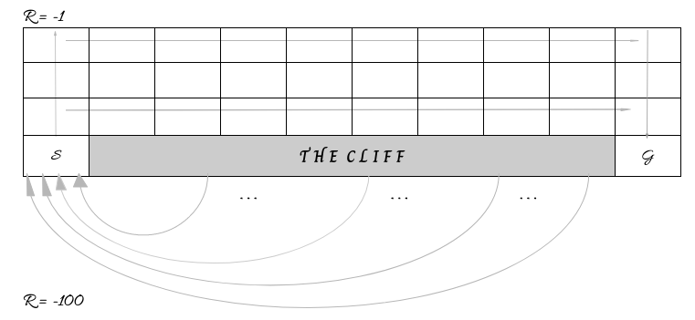
これらの条件下で達成可能な最大報酬は-11（1回上に移動、9回右に移動、1回下に移動）です。負の報酬を使うのは、エージェントにできるだけ早くゴール状態に到達するよう促す一般的な手法です。

セクション2：Qラーニング

チュートリアル開始からここまでの推定所要時間：20分

環境が整ったところで、どうやって解くのでしょうか？

行動価値（Q値）を推定する最も有名なアルゴリズムの一つが、時系列差分（TD）制御アルゴリズムであるQラーニング（Watkins, 1989）です。

Q(s_t,a_t) \leftarrow Q(s_t,a_t) + \alpha \big(r_t + \gamma\max_\limits{a} Q(s_{t+1},a) - Q(s_t,a_t)\big)

ここで、 $Q(s,a)$ は状態 $s$ での行動 $a$ の価値関数、 $\alpha$ は学習率、 $r$ は報酬、 $\gamma$ は時間割引率です。

式中の $r_t + \gamma\max_\limits{a} Q(s_{t+1},a)$ はTDターゲットと呼ばれ、

r_t + \gamma\max_\limits{a} Q(s_{t+1},a) - Q(s_t,a_t),

すなわちTDターゲットと現在のQ値の差はTD誤差、または報酬予測誤差と呼ばれます。

TDターゲットの最大値演算子は最適なQ値を選択するため、Qラーニングはエージェントが現在従っている方策に関係なく、最適な行動価値、すなわち最適に振る舞った場合に得られる将来の累積報酬を直接推定します。このため、Qラーニングはオフポリシー法と呼ばれます。

コーディング演習2：Qラーニングアルゴリズムの実装

この演習では、上記のQラーニング更新則を実装します。引数として、前の状態 $s_t$ 、取った行動 $a_t$ 、得た報酬 $r_t$ 、現在の状態 $s_{t+1}$ 、Q値テーブル、そして学習率 $\alpha$ と割引率 $\gamma$ を含むパラメータ辞書を受け取ります。メソッドは更新されたQ値テーブルを返します。パラメータ辞書では、 $\alpha$ はparams['alpha']、 $\gamma$ はparams['gamma']です。

Qラーニングアルゴリズムができたら、クリフワールド環境を解く学習をどのように行うか見ていきます。

前回のチュートリアルで学んだように、強化学習アルゴリズムの大きな特徴は、活用（exploitation）と探索（exploration）のバランスを取る能力です。Qラーニングエージェントでは、再びイプシロングリーディ戦略を用います。各ステップで、確率 $1 - \epsilon$ で現在の状態における最良の行動（価値関数に基づく）を選び、それ以外はランダムに行動します。

エージェントが環境と相互作用し学習する過程は、ヘルパー関数learn_environmentで処理されます。これは状態観測、行動選択（イプシロングリーディ）、実行、報酬、状態遷移という学習エピソードのライフサイクル全体を実装しています。後でコードを確認して全体の流れを理解しても良いですが、まずはエージェントを試してみましょう。

# @markdown Execute to get helper functions `epsilon_greedy`, `CliffWorld`, and `learn_environment`

def epsilon_greedy(q, epsilon):
  """Epsilon-greedy policy: selects the maximum value action with probability
  (1-epsilon) and selects randomly with epsilon probability.

  Args:
    q (ndarray): an array of action values
    epsilon (float): probability of selecting an action randomly

  Returns:
    int: the chosen action
  """
  if np.random.random() > epsilon:
    action = np.argmax(q)
  else:
    action = np.random.choice(len(q))

  return action


class CliffWorld:
  """
  World: Cliff world.
  40 states (4-by-10 grid world).
  The mapping from state to the grids are as follows:
  30 31 32 ... 39
  20 21 22 ... 29
  10 11 12 ... 19
  0  1  2  ...  9
  0 is the starting state (S) and 9 is the goal state (G).
  Actions 0, 1, 2, 3 correspond to right, up, left, down.
  Moving anywhere from state 9 (goal state) will end the session.
  Taking action down at state 11-18 will go back to state 0 and incur a
      reward of -100.
  Landing in any states other than the goal state will incur a reward of -1.
  Going towards the border when already at the border will stay in the same
      place.
  """
  def __init__(self):
    self.name = "cliff_world"
    self.n_states = 40
    self.n_actions = 4
    self.dim_x = 10
    self.dim_y = 4
    self.init_state = 0

  def get_outcome(self, state, action):
    if state == 9:  # goal state
      reward = 0
      next_state = None
      return next_state, reward
    reward = -1  # default reward value
    if action == 0:  # move right
      next_state = state + 1
      if state % 10 == 9:  # right border
        next_state = state
      elif state == 0:  # start state (next state is cliff)
        next_state = None
        reward = -100
    elif action == 1:  # move up
      next_state = state + 10
      if state >= 30:  # top border
        next_state = state
    elif action == 2:  # move left
      next_state = state - 1
      if state % 10 == 0:  # left border
        next_state = state
    elif action == 3:  # move down
      next_state = state - 10
      if state >= 11 and state <= 18:  # next is cliff
        next_state = None
        reward = -100
      elif state <= 9:  # bottom border
        next_state = state
    else:
      print("Action must be between 0 and 3.")
      next_state = None
      reward = None
    return int(next_state) if next_state is not None else None, reward

  def get_all_outcomes(self):
    outcomes = {}
    for state in range(self.n_states):
      for action in range(self.n_actions):
        next_state, reward = self.get_outcome(state, action)
        outcomes[state, action] = [(1, next_state, reward)]
    return outcomes


def learn_environment(env, learning_rule, params, max_steps, n_episodes):
  # Start with a uniform value function
  value = np.ones((env.n_states, env.n_actions))

  # Run learning
  reward_sums = np.zeros(n_episodes)

  # Loop over episodes
  for episode in range(n_episodes):
    state = env.init_state  # initialize state
    reward_sum = 0

    for t in range(max_steps):
      # choose next action
      action = epsilon_greedy(value[state], params['epsilon'])

      # observe outcome of action on environment
      next_state, reward = env.get_outcome(state, action)

      # update value function
      value = learning_rule(state, action, reward, next_state, value, params)

      # sum rewards obtained
      reward_sum += reward

      if next_state is None:
          break  # episode ends
      state = next_state

    reward_sums[episode] = reward_sum

  return value, reward_sums

def q_learning(state, action, reward, next_state, value, params):
  """Q-learning: updates the value function and returns it.

  Args:
    state (int): the current state identifier
    action (int): the action taken
    reward (float): the reward received
    next_state (int): the transitioned to state identifier
    value (ndarray): current value function of shape (n_states, n_actions)
    params (dict): a dictionary containing the default parameters

  Returns:
    ndarray: the updated value function of shape (n_states, n_actions)
  """
  # Q-value of current state-action pair
  q = value[state, action]

  ##########################################################
  ## TODO for students: implement the Q-learning update rule
  # Fill out function and remove
  raise NotImplementedError("Student exercise: implement the Q-learning update rule")
  ##########################################################

  # write an expression for finding the maximum Q-value at the current state
  if next_state is None:
    max_next_q = 0
  else:
    max_next_q = ...

  # write the expression to compute the TD error
  td_error = ...
  # write the expression that updates the Q-value for the state-action pair
  value[state, action] = ...

  return value


# set for reproducibility, comment out / change seed value for different results
np.random.seed(1)

# parameters needed by our policy and learning rule
params = {
  'epsilon': 0.1,  # epsilon-greedy policy
  'alpha': 0.1,  # learning rate
  'gamma': 1.0,  # discount factor
}

# episodes/trials
n_episodes = 500
max_steps = 1000

# environment initialization
env = CliffWorld()

# solve Cliff World using Q-learning
results = learn_environment(env, q_learning, params, max_steps, n_episodes)
value_qlearning, reward_sums_qlearning = results

# Plot results
plot_performance(env, value_qlearning, reward_sums_qlearning)

解答を見る$

出力例:

# @title Submit your feedback
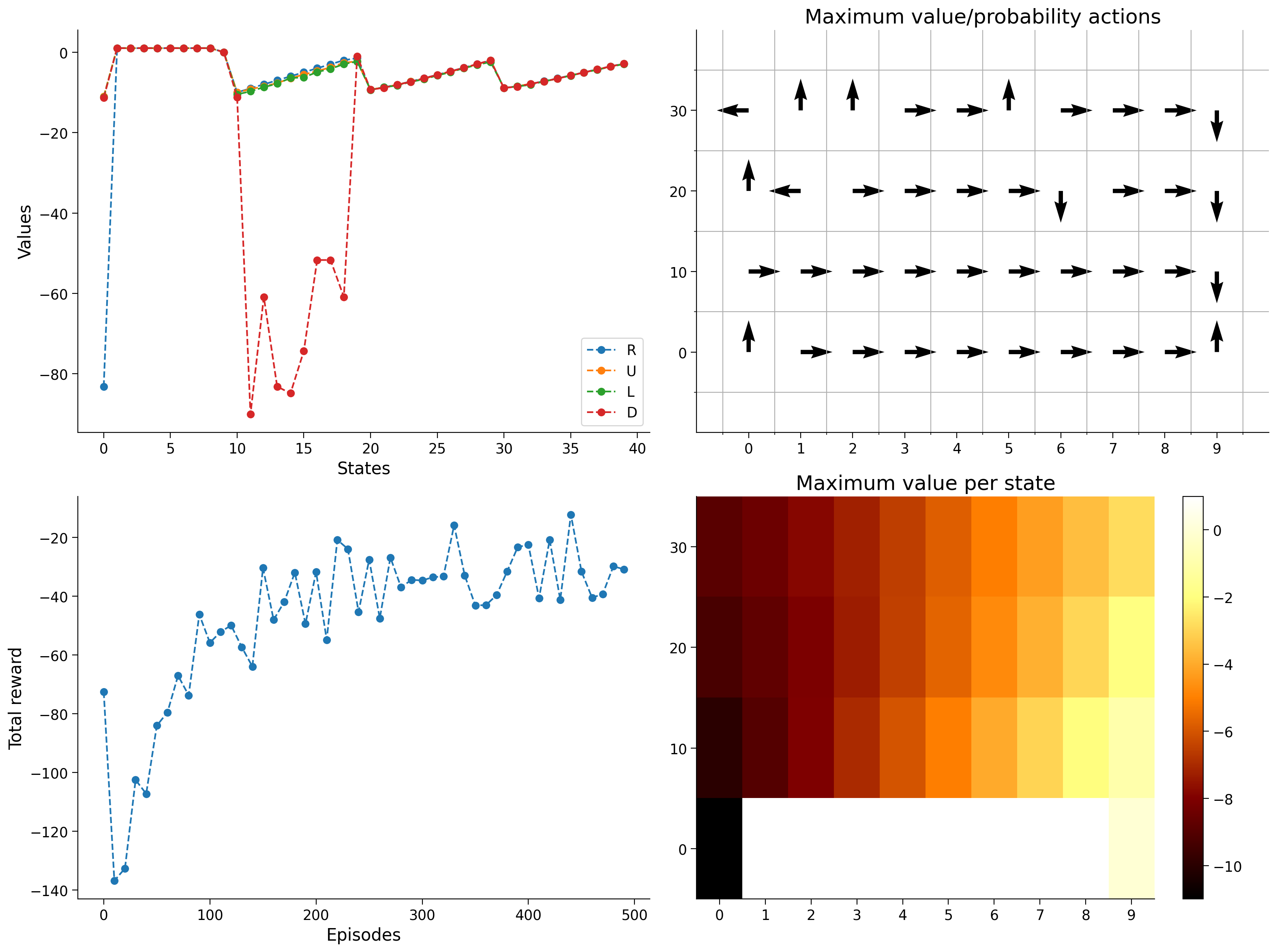
content_review(f"{feedback_prefix}_Implement_Q_learning_algorithm_Exercise")

すべてがうまくいった場合、エージェントの学習と進捗の異なる側面を示す4つのプロットが表示されるはずです。

左上はQテーブル自体の表現で、異なる状態における異なる行動の値を示しています。特に、開始状態から右に行くことや崖の上で下に行くことは明らかに非常に悪いことがわかります。
右上の図はQテーブルに基づくグリーディポリシーを示しており、つまりエージェントがその状態で最善の推測だけを取った場合にどの行動を取るかを示しています。
右下は左上と同じですが、行動を示す代わりに特定の状態における最大Q値の表現を示しています。
左下は実際の学習の証拠であり、各エピソード後に総報酬が着実に増加し、最大可能報酬の-11に漸近しているのが見て取れます。

パラメータやランダムシードを変更して、エージェントの行動がどのように変わるか試してみてください。

まとめ

チュートリアルの推定所要時間：40分

このチュートリアルでは、クリフワールド環境を解決するためにQ学習に基づく強化学習エージェントを実装しました。Q学習は、イプシロングリーディ法による探索と活用のバランスを、テーブルベースの価値関数と組み合わせて、各状態の将来の期待報酬を学習します。

ボーナスセクション1：SARSA

Q学習の代替として、SARSAアルゴリズムも行動価値を推定します。ただし、最適（オフポリシー）値を推定するのではなく、SARSAはオンポリシーの行動価値、つまりエージェントが現在の信念に従って行動した場合に得られる累積将来報酬を推定します。

Q(s_t,a_t) \leftarrow Q(s_t,a_t) + \alpha \big(r_t + \gamma Q(s_{t+1},a_{t+1}) - Q(s_t,a_t)\big)

ここで再び、 $Q(s,a)$ は状態 $s$ での行動 $a$ の価値関数、 $\alpha$ は学習率、 $r$ は報酬、 $\gamma$ は時間割引率です。

実際には、Q学習とSARSAの唯一の違いは、TDターゲットの計算において次の行動を選択する際に（我々の場合はイプシロングリーディ法で）ポリシーを用いるか、Q値を最大化する行動を用いるかの違いです。

ボーナスコーディング演習1：SARSAアルゴリズムの実装

この演習では、上記のSARSA更新ルールを実装します。Q学習と同様に、前の状態 $s_t$ 、取った行動 $a_t$ 、受け取った報酬 $r_t$ 、現在の状態 $s_{t+1}$ 、Q値テーブル、および学習率 $\alpha$ と割引率 $\gamma$ を含むパラメータ辞書を引数として受け取ります。メソッドは更新されたQ値テーブルを返します。次の行動を取得するためにepsilon_greedy関数を使用しても構いません。パラメータ辞書では、 $\alpha$ はparams['alpha']、 $\gamma$ はparams['gamma']、 $\epsilon$ はparams['epsilon']です。

SARSAの実装ができたら、クリフワールドに対してどのように対処するかを見てみましょう。Q学習で試したのと同じセットアップを再度使用します。

def sarsa(state, action, reward, next_state, value, params):
  """SARSA: updates the value function and returns it.

  Args:
    state (int): the current state identifier
    action (int): the action taken
    reward (float): the reward received
    next_state (int): the transitioned to state identifier
    value (ndarray): current value function of shape (n_states, n_actions)
    params (dict): a dictionary containing the default parameters

  Returns:
    ndarray: the updated value function of shape (n_states, n_actions)
  """
  # value of previous state-action pair
  q = value[state, action]

  ##########################################################
  ## TODO for students: implement the SARSA update rule
  # Fill out function and remove
  raise NotImplementedError("Student exercise: implement the SARSA update rule")
  ##########################################################

  # select the expected value at current state based on our policy by sampling
  # from it
  if next_state is None:
    policy_next_q = 0
  else:
    # write an expression for selecting an action using epsilon-greedy
    policy_action = ...
    # write an expression for obtaining the value of the policy action at the
    # current state
    policy_next_q = ...

  # write the expression to compute the TD error
  td_error = ...
  # write the expression that updates the Q-value for the state-action pair
  value[state, action] = ...

  return value


# set for reproducibility, comment out / change seed value for different results
np.random.seed(1)

# parameters needed by our policy and learning rule
params = {
  'epsilon': 0.1,  # epsilon-greedy policy
  'alpha': 0.1,  # learning rate
  'gamma': 1.0,  # discount factor
}

# episodes/trials
n_episodes = 500
max_steps = 1000

# environment initialization
env = CliffWorld()

# learn Cliff World using Sarsa -- uncomment to check your solution!
results = learn_environment(env, sarsa, params, max_steps, n_episodes)
value_sarsa, reward_sums_sarsa = results

# Plot results
plot_performance(env, value_sarsa, reward_sums_sarsa)

def sarsa(state, action, reward, next_state, value, params):
  """SARSA: updates the value function and returns it.

  Args:
    state (int): the current state identifier
    action (int): the action taken
    reward (float): the reward received
    next_state (int): the transitioned to state identifier
    value (ndarray): current value function of shape (n_states, n_actions)
    params (dict): a dictionary containing the default parameters

  Returns:
    ndarray: the updated value function of shape (n_states, n_actions)
  """
  # value of previous state-action pair
  q = value[state, action]

  # select the expected value at current state based on our policy by sampling
  # from it
  if next_state is None:
    policy_next_q = 0
  else:
    # write an expression for selecting an action using epsilon-greedy
    policy_action = epsilon_greedy(value[next_state], params['epsilon'])
    # write an expression for obtaining the value of the policy action at the
    # current state
    policy_next_q = value[next_state, policy_action]

  # write the expression to compute the TD error
  td_error = reward + params['gamma'] * policy_next_q - q
  # write the expression that updates the Q-value for the state-action pair
  value[state, action] = q + params['alpha'] * td_error

  return value


# set for reproducibility, comment out / change seed value for different results
np.random.seed(1)

# parameters needed by our policy and learning rule
params = {
  'epsilon': 0.1,  # epsilon-greedy policy
  'alpha': 0.1,  # learning rate
  'gamma': 1.0,  # discount factor
}

# episodes/trials
n_episodes = 500
max_steps = 1000

# environment initialization
env = CliffWorld()

# learn Cliff World using Sarsa -- uncomment to check your solution!
results = learn_environment(env, sarsa, params, max_steps, n_episodes)
value_sarsa, reward_sums_sarsa = results

# Plot results
with plt.xkcd():
  plot_performance(env, value_sarsa, reward_sums_sarsa)

# @title Submit your feedback
content_review(f"{feedback_prefix}_Implement_the_SARSA_algorithm_Bonus_Exercise")

SARSAもQ学習と似たような結果でタスクを解決することがわかるはずです。注目すべき違いは、SARSAは崖の端でおどおどしているように見え、しばしば崖から離れてから戻ってゴールに向かう傾向があることです。

再度、パラメータやランダムシードを変更して、エージェントの行動がどのように変わるか試してみてください。

ボーナスセクション2：オンポリシー vs オフポリシー

これでオンポリシー学習アルゴリズムとオフポリシー学習アルゴリズムの両方の例を見ました。Q学習とSARSAの報酬結果を並べて比較し、それらがどのように異なるかを見てみましょう。

# @markdown Execute to see visualization

# parameters needed by our policy and learning rule
params = {
  'epsilon': 0.1,  # epsilon-greedy policy
  'alpha': 0.1,  # learning rate
  'gamma': 1.0,  # discount factor
}

# episodes/trials
n_episodes = 500
max_steps = 1000

# environment initialization
env = CliffWorld()

# learn Cliff World using Sarsa
np.random.seed(1)
results = learn_environment(env, q_learning, params, max_steps, n_episodes)
value_qlearning, reward_sums_qlearning = results
np.random.seed(1)
results = learn_environment(env, sarsa, params, max_steps, n_episodes)
value_sarsa, reward_sums_sarsa = results

fig, ax = plt.subplots()
ax.plot(reward_sums_qlearning, label='Q-learning')
ax.plot(reward_sums_sarsa, label='SARSA')
ax.set(xlabel='Episodes', ylabel='Total reward')
plt.legend(loc='lower right')
plt.show(fig)

この単純なクリフワールドタスクでは、Q学習とSARSAはパフォーマンスの観点からほとんど区別がつきませんが、500エピソードの時間範囲内ではQ学習がわずかに優位に見えます。もう一度「グリーディポリシー」の図を見てみましょう。

# @markdown Execute to see visualization

fig, (ax1, ax2) = plt.subplots(ncols=2, figsize=(16, 6))
plot_quiver_max_action(env, value_qlearning, ax=ax1)
ax1.set(title='Q-learning maximum value/probability actions')
plot_quiver_max_action(env, value_sarsa, ax=ax2)
ax2.set(title='SARSA maximum value/probability actions')
plt.show(fig)

すぐに気づくべきことは、Q学習は崖の端をかすめながら上に行き、すぐに右に進み、壁にぶつかってから下に行きゴールに到達するポリシーを学習したことです。崖から離れたポリシーは不確かさが高いです。

一方、SARSAは崖の端を避け、ゴール側に向かう前にもう一つ上のタイルに行くように見えます。これも明らかにゴールに到達する課題を解決していますが、真に最適なルートよりも-2の追加コストがかかっています。

なぜこれらの行動がこのように現れたと思いますか？