![]()

チュートリアル 1: 予測を学習する
第3週4日目: 強化学習
Neuromatch Academy 提供
コンテンツ制作者: Marcelo G Mattar, Eric DeWitt, Matt Krause, Matthew Sargent, Anoop Kulkarni, Sowmya Parthiban, Feryal Behbahani, Jane Wang
コンテンツレビュアー: Ella Batty, Byron Galbraith, Michael Waskom, Ezekiel Williams, Mehul Rastogi, Lily Cheng, Roberto Guidotti, Arush Tagade, Kelson Shilling-Scrivo
制作編集者: Gagana B, Spiros Chavlis
チュートリアルの目的
推定所要時間: 50分
強化学習(Reinforcement Learning, RL)は、エージェントが報酬を最大化する行動を学習する問題を定義し解決するための枠組みです。問題の設定は次の通りです:生物的または人工的なエージェントが現在の世界の状態を観察し、その状態に基づいて行動を選択します。行動を実行すると、エージェントは報酬を受け取り、この情報を使って将来の行動を改善します。強化学習は学習の形式的かつ最適な記述を提供します。これらの記述は最初に動物行動の研究から導かれ、その後モデルで使われる形式的な量が人間や動物の脳内で観察されることで検証されました。
強化学習は広範な枠組みであり、NMAで扱う多くのトピックと深い関連があります。例えば、ほとんどの強化学習は世界をマルコフ決定問題(Markov Decision Problem)として定義しており、これは隠れた動的システム(Hidden Dynamics)や最適制御(Optimal Control)に基づいています。より広く見ると、強化学習は経済学、心理学、計算機科学、人工知能など他分野の多くのアイデアや形式を取り入れて、単純な報酬信号だけで大規模かつ複雑な問題を解くアルゴリズムやモデルを定義できる枠組みと見なせます。
このチュートリアルでは、エージェントを将来の報酬を予測する観察者としてモデル化します。このエージェントは行動を取らず、したがって受け取る報酬の量に影響を与えられません。各状態に続く報酬の量を予測することで、エージェントは世界の中で最も報酬が多く続く傾向にある最良の状態を特定できるようになります。
より具体的には、古典的条件付けパラダイムで状態価値関数を推定する方法を学び、時間差(Temporal Difference, TD)学習を用いて条件刺激(CS)と無条件刺激(US)の提示時におけるTD誤差を異なるCS-USの連関条件下で調べます。これらの演習を通じて、古典的条件付けにおける報酬予測誤差(RPE)の振る舞いと、ドーパミンが「標準的な」モデルフリーRPEを表現している場合に期待されることを理解できます。
このチュートリアルの終わりには:
- 標準的なタップドディレイライン条件付けモデルの使い方を学びます
- RPEがCSに移動する仕組みを理解します
- 報酬サイズの変動がRPEに与える影響を理解します
- US-CSのタイミングの違いがRPEに与える影響を理解します
チュートリアル1~4の完了には3時間以上かかる見込みですが、この内容に全く馴染みがない場合や追加資料をすべて学習したい場合はさらに時間がかかることがあります。
# @title Tutorial slides
# @markdown These are the slides for all videos in this tutorial.
from IPython.display import IFrame
link_id = "2jzdu"
print(f"If you want to download the slides: https://osf.io/download/{link_id}/")
IFrame(src=f"https://mfr.ca-1.osf.io/render?url=https://osf.io/{link_id}/?direct%26mode=render%26action=download%26mode=render", width=854, height=480)
セットアップ
# @title Install and import feedback gadget


from vibecheck import DatatopsContentReviewContainer
def content_review(notebook_section: str):
    return DatatopsContentReviewContainer(
        "",  # No text prompt
        notebook_section,
        {
            "url": "https://pmyvdlilci.execute-api.us-east-1.amazonaws.com/klab",
            "name": "neuromatch_cn",
            "user_key": "y1x3mpx5",
        },
    ).render()


feedback_prefix = "W3D4_T1"
# Imports
import numpy as np
import matplotlib.pyplot as plt# @title Figure Settings
import logging
logging.getLogger('matplotlib.font_manager').disabled = True
import ipywidgets as widgets # interactive display
%config InlineBackend.figure_format = 'retina'
plt.style.use("https://raw.githubusercontent.com/NeuromatchAcademy/course-content/main/nma.mplstyle")# @title Plotting Functions
from matplotlib import ticker
def plot_value_function(V, ax=None, show=True):
"""Plot V(s), the value function"""
if not ax:
fig, ax = plt.subplots()
ax.stem(V)
ax.set_ylabel('Value')
ax.set_xlabel('State')
ax.set_title("Value function: $V(s)$")
if show:
plt.show()
def plot_tde_trace(TDE, ax=None, show=True, skip=400):
"""Plot the TD Error across trials"""
if not ax:
fig, ax = plt.subplots()
index = np.arange(0, TDE.shape[1], skip)
im = ax.imshow(TDE[:,index])
positions = ax.get_xticks()
# Avoid warning when setting string tick labels
ax.xaxis.set_major_locator(ticker.FixedLocator(positions))
ax.set_xticklabels([f"{int(skip * x)}" for x in positions])
ax.set_title('TD-error over learning')
ax.set_ylabel('State')
ax.set_xlabel('Iterations')
ax.figure.colorbar(im)
if show:
plt.show()
def learning_summary_plot(V, TDE):
"""Summary plot for Ex1"""
fig, (ax1, ax2) = plt.subplots(nrows = 2, gridspec_kw={'height_ratios': [1, 2]})
plot_value_function(V, ax=ax1, show=False)
plot_tde_trace(TDE, ax=ax2, show=False)
plt.tight_layout()
plt.show()# @title Helper Functions and Classes
def reward_guesser_title_hint(r1, r2):
""""Provide a mildly obfuscated hint for a demo."""
if (r1==14 and r2==6) or (r1==6 and r2==14):
return "Technically correct...(the best kind of correct)"
if ~(~(r1+r2) ^ 11) - 1 == (6 | 24): # Don't spoil the fun :-)
return "Congratulations! You solved it!"
return "Keep trying...."
class ClassicalConditioning:
def __init__(self, n_steps, reward_magnitude, reward_time):
# Task variables
self.n_steps = n_steps
self.n_actions = 0
self.cs_time = int(n_steps/4) - 1
# Reward variables
self.reward_state = [0,0]
self.reward_magnitude = None
self.reward_probability = None
self.reward_time = None
# Time step at which the conditioned stimulus is presented
self.set_reward(reward_magnitude, reward_time)
# Create a state dictionary
self._create_state_dictionary()
def set_reward(self, reward_magnitude, reward_time):
"""
Determine reward state and magnitude of reward
"""
if reward_time >= self.n_steps - self.cs_time:
self.reward_magnitude = 0
else:
self.reward_magnitude = reward_magnitude
self.reward_state = [1, reward_time]
def get_outcome(self, current_state):
"""
Determine next state and reward
"""
# Update state
if current_state < self.n_steps - 1:
next_state = current_state + 1
else:
next_state = 0
# Check for reward
if self.reward_state == self.state_dict[current_state]:
reward = self.reward_magnitude
else:
reward = 0
return next_state, reward
def _create_state_dictionary(self):
"""
This dictionary maps number of time steps/ state identities
in each episode to some useful state attributes:
state - 0 1 2 3 4 5 (cs) 6 7 8 9 10 11 12 ...
is_delay - 0 0 0 0 0 0 (cs) 1 1 1 1 1 1 1 ...
t_in_delay - 0 0 0 0 0 0 (cs) 1 2 3 4 5 6 7 ...
"""
d = 0
self.state_dict = {}
for s in range(self.n_steps):
if s <= self.cs_time:
self.state_dict[s] = [0,0]
else:
d += 1 # Time in delay
self.state_dict[s] = [1,d]
class MultiRewardCC(ClassicalConditioning):
"""Classical conditioning paradigm, except that one randomly selected reward,
magnitude, from a list, is delivered of a single fixed reward."""
def __init__(self, n_steps, reward_magnitudes, reward_time=None):
""""Build a multi-reward classical conditioning environment
Args:
- nsteps: Maximum number of steps
- reward_magnitudes: LIST of possible reward magnitudes.
- reward_time: Single fixed reward time
Uses numpy global random state.
"""
super().__init__(n_steps, 1, reward_time)
self.reward_magnitudes = reward_magnitudes
def get_outcome(self, current_state):
next_state, reward = super().get_outcome(current_state)
if reward:
reward=np.random.choice(self.reward_magnitudes)
return next_state, reward
class ProbabilisticCC(ClassicalConditioning):
"""Classical conditioning paradigm, except that rewards are stochastically omitted."""
def __init__(self, n_steps, reward_magnitude, reward_time=None, p_reward=0.75):
""""Build a multi-reward classical conditioning environment
Args:
- nsteps: Maximum number of steps
- reward_magnitudes: Reward magnitudes.
- reward_time: Single fixed reward time.
- p_reward: probability that reward is actually delivered in rewarding state
Uses numpy global random state.
"""
super().__init__(n_steps, reward_magnitude, reward_time)
self.p_reward = p_reward
def get_outcome(self, current_state):
next_state, reward = super().get_outcome(current_state)
if reward:
reward*= int(np.random.uniform(size=1)[0] < self.p_reward)
return next_state, rewardセクション1: 時間差学習
# @title Video 1: Introduction
from ipywidgets import widgets
from IPython.display import YouTubeVideo
from IPython.display import IFrame
from IPython.display import display


class PlayVideo(IFrame):
  def __init__(self, id, source, page=1, width=400, height=300, **kwargs):
    self.id = id
    if source == 'Bilibili':
      src = f'https://player.bilibili.com/player.html?bvid={id}&page={page}'
    elif source == 'Osf':
      src = f'https://mfr.ca-1.osf.io/render?url=https://osf.io/download/{id}/?direct%26mode=render'
    super(PlayVideo, self).__init__(src, width, height, **kwargs)


def display_videos(video_ids, W=400, H=300, fs=1):
  tab_contents = []
  for i, video_id in enumerate(video_ids):
    out = widgets.Output()
    with out:
      if video_ids[i][0] == 'Youtube':
        video = YouTubeVideo(id=video_ids[i][1], width=W,
                             height=H, fs=fs, rel=0)
        print(f'Video available at https://youtube.com/watch?v={video.id}')
      else:
        video = PlayVideo(id=video_ids[i][1], source=video_ids[i][0], width=W,
                          height=H, fs=fs, autoplay=False)
        if video_ids[i][0] == 'Bilibili':
          print(f'Video available at https://www.bilibili.com/video/{video.id}')
        elif video_ids[i][0] == 'Osf':
          print(f'Video available at https://osf.io/{video.id}')
      display(video)
    tab_contents.append(out)
  return tab_contents


video_ids = [('Youtube', 'YoNbc9M92YY'), ('Bilibili', 'BV13f4y1d7om')]
tab_contents = display_videos(video_ids, W=854, H=480)
tabs = widgets.Tab()
tabs.children = tab_contents
for i in range(len(tab_contents)):
  tabs.set_title(i, video_ids[i][0])
display(tabs)
# @title Submit your feedback
content_review(f"{feedback_prefix}_Introduction_Video")環境:
- エージェントは環境をエピソード(試行とも呼ばれる)として体験します。
- エピソードはインタートライアルインターバル(ITI)状態への遷移によって終了し、またITI状態から開始されます。終端状態およびITI状態の値はゼロに固定します。
- 古典的条件付け環境は、エージェントが決定論的に遷移する一連の状態で構成されます。状態0から開始し、最初のステップで状態1へ、次に状態1から状態2へと進みます。これらの状態は「タップ遅延線」表現と呼ばれる時間を表しています。
- 各エピソード内で、エージェントにはCS(手がかり)とUS(報酬)が提示されます。
- CS(手がかり)は試行の最初の4分の1の終わりに提示され、US(報酬)はその直後に与えられます。CSとUSの間隔は
reward_timeで指定されます。 - エージェントの目標は、試行中の各状態から期待される報酬を予測することを学習することです。
一般的な概念
参考文献: McClelland, J. L., Rumelhart, D. E. (1989). Explorations in parallel distributed processing: A handbook of models, programs, and exercises. Chapter 9, MIT press. URL: web.stanford.edu/group/pdplab/pdphandbook/handbookch10.html
- リターン : 時刻 における将来の累積報酬:
ここで は時刻 に受け取る報酬の量、 は将来の報酬の現在における重要度を示す割引率です。
リターン は再帰的な形でも表せます:
-
状態 は現在の状態や状況を表し、通常はエージェントが環境から得る観測から得られます。
-
方策 はエージェントの行動の仕様を示します。 は状態 にいるときに行動 をとる確率を表します。
-
価値関数 は状態 から始めて方策 に従って行動したときの期待リターンとして定義されます。大まかに言えば、価値関数は方策 に従ったときに状態 にいることが「どれだけ良いか」を推定します。
\begin{align}
V_{\pi}(s_t=s) &= [ $G_{t}$; | ; s_t=s, a_{t:\infty}\sim\pi] \
& = [ + ; | ; s_t=s, a_{t:\infty}\sim\pi]
\end{align} -
これらを組み合わせると、
\begin{align}
V_{\pi}(s_t=s) &= [ + ; | ; s_t=s, a_{t:\infty}\sim\pi] \
&= $\sum_a \pi(a|s) \sum_{r, s'}p(s', r)(r + V_{\pi}(s_{t+1}=s'))
\end{align}
$時系列差分(TD)学習
-
マルコフ性の仮定のもとで、 を真のリターン の代理として使えます。これにより、TD誤差を計算する一般化された式が得られます:
\begin{align}
$\delta_{t} = r_{t+1} + \gamma V(s_{t+1}) - V(s_{t})
\end{align} -
TD$誤差は時刻 と の価値の差異を測ります。TD誤差を計算したら、価値の差異を減らすために「価値の更新」を行います:
\begin{align}
$\leftarrow V(s_{t}) + \alpha \delta_{t}
\end{align}
*$ 差異をどれだけ速く減らすかは定数(ハイパーパラメータ)(学習率)で指定されます。
定義(要約):
- リターン:
- TD誤差:
- 価値の更新:
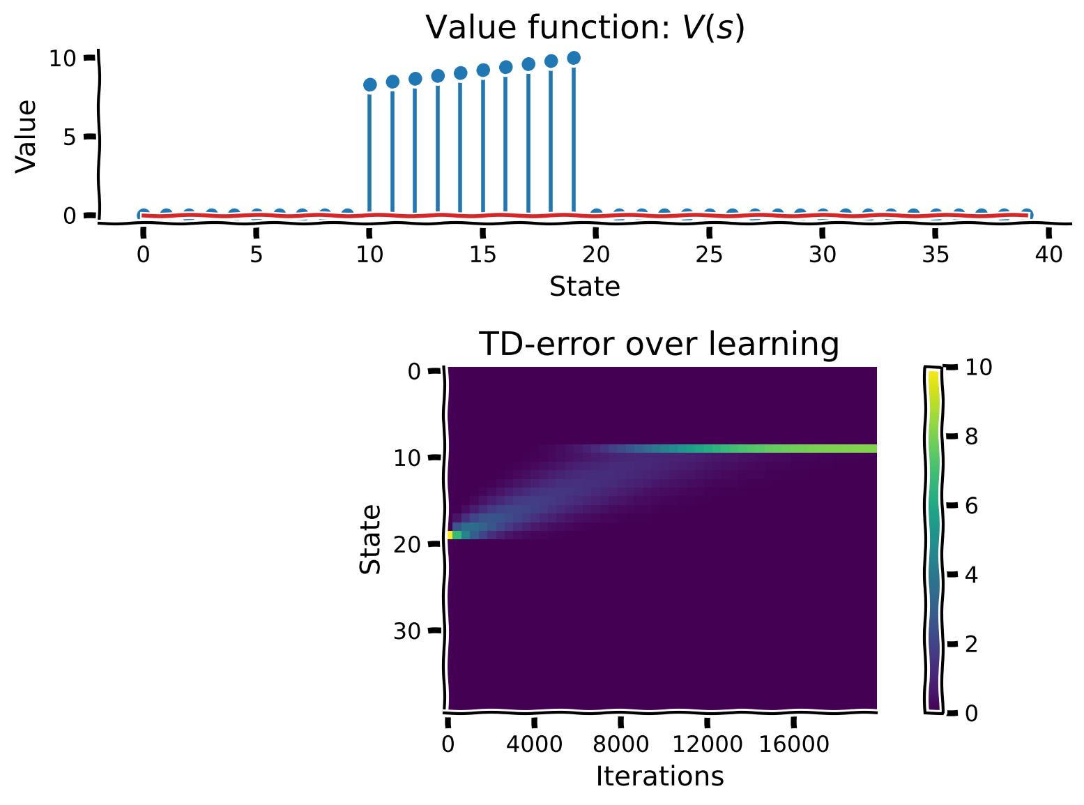
コーディング演習 1: 報酬が保証されたTD学習
この演習では、古典的条件付けパラダイムにおける状態価値関数を推定するためにTD学習を実装します。報酬は固定の大きさで、条件刺激(CS)の後に固定の遅延で与えられます。学習中(試行を通じて)のTD誤差を保存して、後で可視化できるようにしてください。
CSの効果をシミュレートするために、CS後の遅延期間中のみ を更新すべきです。この期間はブール変数 is_delay で示されます。価値関数の更新式に is_delay を掛けることで実装できます。
提供されたコードを使って価値関数を推定してください。ヘルパークラス ClassicalConditioning を使用します。
def td_learner(env, n_trials, gamma=0.98, alpha=0.001):
  """ Temporal Difference learning

  Args:
    env (object): the environment to be learned
    n_trials (int): the number of trials to run
    gamma (float): temporal discount factor
    alpha (float): learning rate

  Returns:
    ndarray, ndarray: the value function and temporal difference error arrays
  """
  V = np.zeros(env.n_steps) # Array to store values over states (time)
  TDE = np.zeros((env.n_steps, n_trials)) # Array to store TD errors

  for n in range(n_trials):

    state = 0 # Initial state

    for t in range(env.n_steps):

      # Get next state and next reward
      next_state, reward = env.get_outcome(state)

      # Is the current state in the delay period (after CS)?
      is_delay = env.state_dict[state][0]

      ########################################################################
      ## TODO for students: implement TD error and value function update
      # Fill out function and remove
      raise NotImplementedError("Student exercise: implement TD error and value function update")
      #################################################################################
      # Write an expression to compute the TD-error
      TDE[state, n] = ...

      # Write an expression to update the value function
      V[state] += ...

      # Update state
      state = next_state

  return V, TDE


# Initialize classical conditioning class
env = ClassicalConditioning(n_steps=40, reward_magnitude=10, reward_time=10)

# Perform temporal difference learning
V, TDE = td_learner(env, n_trials=20000)

# Visualize
learning_summary_plot(V, TDE)出力例:
# @title Submit your feedback
content_review(f"{feedback_prefix}_TD_learning_Exercise")
インタラクティブデモ 1.1: USからCSへの転移
古典的条件付けの過程で、被験者の行動反応(例えばよだれ)は無条件刺激(US; おいしい食べ物の匂いなど)から、それを予測する条件刺激(CS; パブロフのベルの音など)へと移ります。報酬予測誤差は、この過程で状態の価値を期待割引リターンに応じて調整する重要な役割を果たします。
TD誤差は以下の式で与えられます:
遅延期間は報酬がゼロなので、学習段階を通じてTD誤差は と の不一致から生じます(この例では割引率はゼロに設定されています)。ある時点のTD誤差が減少すると、その前の時点のTD誤差が増加します。したがって、学習を通じてTD誤差は時間的に逆方向へ移動する傾向があります。
以下のウィジェットを使って、報酬予測誤差が時間とともにどのように変化するかを調べてみましょう。
学習前(オレンジ線)では報酬状態のみが高い報酬予測誤差(青線)を持っています。学習が進むにつれて(スライダー操作)、報酬予測誤差は条件刺激に移動し、試行終了時にはそこに集中します(緑線)。
ドーパミンニューロンは、報酬予測誤差を体内で伝達していると考えられており、まさに同じ挙動を示します!
# @markdown Make sure you execute this cell to enable the widget!

n_trials = 20000

@widgets.interact
def plot_tde_by_trial(trial = widgets.IntSlider(value=5000, min=0, max=n_trials-1 , step=1, description="Trial #")):
  if 'TDE' not in globals():
    print("Complete Exercise 1 to enable this interactive demo!")
  else:

    fig, ax = plt.subplots()
    ax.axhline(0, color='k') # Use this + basefmt=' ' to keep the legend clean.
    ax.stem(TDE[:, 0], linefmt='C1-', markerfmt='C1d', basefmt=' ',
            label="Before Learning (Trial 0)")
    ax.stem(TDE[:, -1], linefmt='C2-', markerfmt='C2s', basefmt=' ',
            label=r"After Learning (Trial $\infty$)")
    ax.stem(TDE[:, trial], linefmt='C0-', markerfmt='C0o', basefmt=' ',
            label=f"Trial {trial}")

    ax.set_xlabel("State in trial")
    ax.set_ylabel("TD Error")
    ax.set_title("Temporal Difference Error by Trial")
    ax.legend()
    plt.show()
# @title Submit your feedback
content_review(f"{feedback_prefix}_US_to_CS_transfer_Interactive_Demo")インタラクティブデモ 1.2: 学習率と割引率
我々のTD学習エージェントには、学習を制御する2つのパラメータがあります。(学習率)と(割引率)です。演習1ではこれらを 、 に設定しました。ここでは、これらのパラメータを変化させるとTD学習が学習するモデルにどのような影響があるかを調べます。
以下のインタラクティブデモを使う前に、これら2つのパラメータの役割について考えてみてください。 は各TD誤差によって生じる価値関数の更新量を制御します。我々の単純で決定論的な世界では、これは最終的に学習されるモデルに影響を与えるでしょうか?より複雑で現実的な環境では、より大きな が必ずしも良いとは限らないでしょうか?
割引率 は将来のリターンに指数関数的に減衰する重みをかけます。これが学習されるモデルにどのように影響するでしょうか? や の場合はどうなるでしょうか?
ウィジェットを使って仮説を検証してみましょう。
# @markdown Make sure you execute this cell to enable the widget!

@widgets.interact
def plot_summary_alpha_gamma(alpha=widgets.FloatSlider(value=0.0001, min=0.0001,
                                                       max=0.1, step=0.0001,
                                                       readout_format='.4f',
                                                       description="alpha"),
                             gamma=widgets.FloatSlider(value=0.980, min=0,
                                                       max=1.1, step=0.010,\
                                                       description="γ")):
  env = ClassicalConditioning(n_steps=40, reward_magnitude=10, reward_time=10)
  try:
    V_params, TDE_params = td_learner(env, n_trials=20000, gamma=gamma,
                                      alpha=alpha)
  except NotImplementedError:
    print("Finish Exercise 1 to enable this interactive demo")

learning_summary_plot(V_params,TDE_params)# @title Submit your feedback
content_review(f"{feedback_prefix}_Learning_rates_and_discount_factors_Interactive_Demo_and_Discussion")セクション 2: 報酬の大きさが変動するTD学習
チュートリアル開始からここまでの推定所要時間: 30分
前の演習では、環境はできるだけ単純でした。各試行で、条件刺激(CS)は同じ報酬を同じタイミングで、100%の確率で予測していました。次のいくつかの演習では、環境を徐々に複雑にし、TD学習者の挙動を調べていきます。
インタラクティブデモ 2: 価値関数を一致させる
まず、環境を複数の報酬のうちランダムに1つを与えるものに置き換えます。下に示すのは、CSが6単位または14単位の報酬を予測し、両方の報酬が同じ確率で与えられる環境で訓練されたTD学習者の最終的な価値関数 です。
同じ価値関数を学習させる別の報酬の組み合わせを見つけられますか?各報酬は50%の確率で与えられると仮定してください。
ヒント:
- 価値関数 の定義をよく考えてください。これは解析的に解くことができます。
- や を変更する必要はありません。
- ランダム性のため、わずかな変動があるかもしれません。
# @markdown Make sure you execute this cell to enable the widget!

# @markdown Please allow some time for the new figure to load

n_trials = 20000
np.random.seed(2020)
rng_state = np.random.get_state()
env = MultiRewardCC(40, [6, 14], reward_time=10)
V_multi, TDE_multi = td_learner(env, n_trials, gamma=0.98, alpha=0.001)

@widgets.interact
def reward_guesser_interaction(r1 = widgets.IntText(value=0, min=0, max=50, description="Reward 1"),
                               r2 = widgets.IntText(value=0, min=0, max=50, description="Reward 2")):
  try:
    env2 = MultiRewardCC(40, [r1, r2], reward_time=10)
    V_guess, _ = td_learner(env2, n_trials, gamma=0.98, alpha=0.001)
    fig, ax = plt.subplots()
    m, l, _ = ax.stem(V_multi, linefmt='y-', markerfmt='yo',
                      basefmt=' ', label="Target")
    m.set_markersize(15)
    m.set_markerfacecolor('none')
    l.set_linewidth(4)
    m, _, _ = ax.stem(V_guess, linefmt='r', markerfmt='rx',
                      basefmt=' ', label="Guess")
    m.set_markersize(15)

    ax.set_xlabel("State")
    ax.set_ylabel("Value")
    ax.set_title(f"Guess V(s)\n{reward_guesser_title_hint(r1, r2)}")
    ax.legend()
    plt.show()
  except NotImplementedError:
    print("Please finish Exercise 1 first!")
考えてみよう! 2: TD誤差の検証
以下のセルを実行して、複数報酬環境でのTD誤差をプロットします。このプロットに新しい特徴が現れています。何でしょうか?なぜ起こるのでしょう?
# @markdown Execute the cell
plot_tde_trace(TDE_multi)# @title Submit your feedback
content_review(f"{feedback_prefix}_Examining_the_TD_Error_Discussion")セクション 3: 確率的報酬によるTD学習
チュートリアル開始からここまでの推定所要時間: 40分
考えてみよう! 3: 確率的報酬
この環境では、再び10単位の単一報酬を与えます。ただし、間欠的に与えられます。20%の試行ではCSが提示されても通常の報酬は与えられず、残りの80%は通常通り報酬が与えられます。
以下のセルを実行してシミュレーションしてください。ノートブックの前半で、決定論的環境では を変えても学習にほとんど影響がないことを見ました。ここでは が1に設定されています。確率的報酬環境で学習率がこれほど大きいとどうなるでしょうか?収束すると思いますか?
高い学習率では、価値関数は観測された報酬に素早く追従し、報酬予測誤差があるたびに急激に変化します。確率的な場合、この挙動は価値関数が変動しすぎて安定(収束)しない原因となります。低い学習率を使うと、報酬信号の変動を平滑化して価値関数を安定させ、時間をかけて平均報酬に収束させることができます。ただし、学習は遅くなります。
最良の結果を得るために、学習の初期段階では高い学習率を使って速く学習し、学習が進むにつれて学習率を徐々に下げて価値関数を平均報酬に収束させる方法がよく使われます。これを「学習率スケジュール」と呼びます。
# @markdown Execute this cell to visualize the value function and TD-errors when `alpha=1`
np.random.set_state(rng_state)  # Resynchronize everyone's notebooks
n_trials = 20000
try:
  env = ProbabilisticCC(n_steps=40, reward_magnitude=10, reward_time=10,
                        p_reward=0.8)
  V_stochastic, TDE_stochastic = td_learner(env, n_trials*2, alpha=1)
  learning_summary_plot(V_stochastic, TDE_stochastic)
except NotImplementedError:
  print("Please finish Exercise 1 first")
# @markdown Execute this cell to visualize the value function and TD-errors when `alpha=0.2`
np.random.set_state(rng_state) # Resynchronize everyone's notebooks
n_trials = 20000
try:
env = ProbabilisticCC(n_steps=40, reward_magnitude=10, reward_time=10,
p_reward=0.8)
V_stochastic, TDE_stochastic = td_learner(env, n_trials*2, alpha=.2)
learning_summary_plot(V_stochastic, TDE_stochastic)
except NotImplementedError:
print("Please finish Exercise 1 first")# @title Submit your feedback
content_review(f"{feedback_prefix}_Probabilistic_rewards_Discussion")まとめ
チュートリアルの推定所要時間: 50分
このノートブックでは、単純なTD学習者を構築し、訓練中の状態表現や報酬予測誤差の変化を調べました。環境やパラメータ(, )を操作することで、その挙動の直感を養いました。
この単純なモデルは、古典的条件付け課題を受ける被験者の行動や、その背後にあると考えられるドーパミン神経細胞の挙動に非常に似ています。TDリセットを実装したり、一般的な実験誤差を再現したかもしれません。ここで使った更新則は、70年以上$にわたり、人工的および生物学的学習の説明として広く研究されています。
しかし、このノートブックには何かが欠けていることに気づいたかもしれません。各状態の価値を慎重に計算しましたが、それを実際に何かに使ってはいません。価値を使って_行動_を計画することは次に学びます!
ボーナス
ボーナス考えてみよう! 1: CSを取り除く
コーディング演習1では、条件刺激に依存する項を含めたはずです。それを取り除いてみてください。何が起こるでしょうか?なぜそうなるのか理解できますか?
この現象は動物の訓練を試みる人をよく惑わしますので注意してください!
# @title Submit your feedback
content_review(f"{feedback_prefix}_Removing_the_CS_Bonus_Discussion")