ボーナスチュートリアル4: カルマンフィルター パート2

第3週 第3日目: 隠れた動力学

Neuromatch Academyによる

コンテンツ作成者: Caroline Haimerl と Byron Galbraith

コンテンツレビュアー: Jesse Livezey, Matt Krause, Michael Waskom, Xaq Pitkow

制作編集: Gagana B, Spiros Chavlis

重要な注意: これはNMA 2020からのボーナスマテリアルであり、大幅な改訂はされていません。したがって、表記や基準がやや異なります。ここに含めているのは、2次元でのカルマンフィルターの動作について追加情報を提供するためです。

参考文献:

• Roweis, Ghahramani (1998): 線形ガウスモデルの統一的レビュー
• Bishop (2006): パターン認識と機械学習

謝辞:

このチュートリアルは、ニューヨーク大学データサイエンスセンターのCristina Savin博士のProbabilistic Time SeriesクラスのためにCaroline Haimerlが作成したコードを一部基にしています

チュートリアルの目的

前回のチュートリアルでは1次元のカルマンフィルターの直感を得ました。今回のチュートリアルでは、2次元カルマンフィルターとその数学的基礎をさらに詳しく見ていきます。

このチュートリアルで学ぶこと:

• 線形動的システムの復習
• カルマンフィルターの実装
• 眼球追跡実験のデータをカルマンフィルターで平滑化する方法の探求

# @title Tutorial slides
# @markdown These are the slides for videos in Bonus tutorials
from IPython.display import IFrame
link_id = "rh23s"
print(f"If you want to download the slides: https://osf.io/download/{link_id}/")
IFrame(src=f"https://mfr.ca-1.osf.io/render?url=https://osf.io/{link_id}/?direct%26mode=render%26action=download%26mode=render", width=854, height=480)

セットアップ

# @title Install dependencies

# @title Install and import feedback gadget


from vibecheck import DatatopsContentReviewContainer
def content_review(notebook_section: str):
    return DatatopsContentReviewContainer(
        "",  # No text prompt
        notebook_section,
        {
            "url": "https://pmyvdlilci.execute-api.us-east-1.amazonaws.com/klab",
            "name": "neuromatch_cn",
            "user_key": "y1x3mpx5",
        },
    ).render()


feedback_prefix = "W3D2_T4_Bonus"

# Imports
import sys
import numpy as np
import matplotlib.pyplot as plt
import pykalman
from scipy import stats

# @title Figure settings
import logging
logging.getLogger('matplotlib.font_manager').disabled = True

import ipywidgets as widgets  # interactive display
%config InlineBackend.figure_format = 'retina'
plt.style.use("https://raw.githubusercontent.com/NeuromatchAcademy/course-content/main/nma.mplstyle")

# @title Plotting functions
np.set_printoptions(precision=3)


def plot_kalman(state, observation, estimate=None, label='filter', color='r-',
                title='LDS', axes=None):
  if axes is None:
    fig, (ax1, ax2) = plt.subplots(ncols=2, figsize=(16, 6))
    ax1.plot(state[:, 0], state[:, 1], 'g-', label='true latent')
    ax1.plot(observation[:, 0], observation[:, 1], 'k.', label='data')
  else:
    ax1, ax2 = axes

  if estimate is not None:
    ax1.plot(estimate[:, 0], estimate[:, 1], color=color, label=label)
  ax1.set(title=title, xlabel='X position', ylabel='Y position')
  ax1.legend()

  if estimate is None:
    ax2.plot(state[:, 0], observation[:, 0], '.k', label='dim 1')
    ax2.plot(state[:, 1], observation[:, 1], '.', color='grey', label='dim 2')
    ax2.set(title='correlation', xlabel='latent', ylabel='measured')
  else:
    ax2.plot(state[:, 0], estimate[:, 0], '.', color=color,
              label='latent dim 1')
    ax2.plot(state[:, 1], estimate[:, 1], 'x', color=color,
              label='latent dim 2')
    ax2.set(title='correlation',
            xlabel='real latent',
            ylabel='estimated latent')
  ax2.legend()
  plt.show()
  return ax1, ax2


def plot_gaze_data(data, img=None, ax=None):
  # overlay gaze on stimulus
  if ax is None:
    fig, ax = plt.subplots(figsize=(8, 6))

  xlim = None
  ylim = None
  if img is not None:
    ax.imshow(img, aspect='auto')
    ylim = (img.shape[0], 0)
    xlim = (0, img.shape[1])

  ax.scatter(data[:, 0], data[:, 1], c='m', s=100, alpha=0.7)
  ax.set(xlim=xlim, ylim=ylim)

  return ax


def plot_kf_state(kf, data, ax, show=True):
  mu_0 = np.ones(kf.n_dim_state)
  mu_0[:data.shape[1]] = data[0]
  kf.initial_state_mean = mu_0

  mu, sigma = kf.smooth(data)
  ax.plot(mu[:, 0], mu[:, 1], 'limegreen', linewidth=3, zorder=1)
  ax.scatter(mu[0, 0], mu[0, 1], c='orange', marker='>', s=200, zorder=2)
  ax.scatter(mu[-1, 0], mu[-1, 1], c='orange', marker='s', s=200, zorder=2)
  if show:
    plt.show()

#@title Data retrieval and loading
import io
import os
import hashlib
import requests

fname = "W2D3_mit_eyetracking_2009.npz"
url = "https://osf.io/jfk8w/download"
expected_md5 = "20c7bc4a6f61f49450997e381cf5e0dd"

if not os.path.isfile(fname):
  try:
    r = requests.get(url)
  except requests.ConnectionError:
    print("!!! Failed to download data !!!")
  else:
    if r.status_code != requests.codes.ok:
      print("!!! Failed to download data !!!")
    elif hashlib.md5(r.content).hexdigest() != expected_md5:
      print("!!! Data download appears corrupted !!!")
    else:
      with open(fname, "wb") as fid:
        fid.write(r.content)

def load_eyetracking_data(data_fname=fname):

  with np.load(data_fname, allow_pickle=True) as dobj:
    data = dict(**dobj)

  images = [plt.imread(io.BytesIO(stim), format='JPG')
            for stim in data['stimuli']]
  subjects = data['subjects']

  return subjects, images

セクション0: はじめに

#@title Video 1: Introduction
# Insert the ID of the corresponding youtube video
from IPython.display import YouTubeVideo
video = YouTubeVideo(id="6f_51L3i5aQ", width=854, height=480, fs=1)
print("Video available at https://youtu.be/" + video.id)
video

# @title Submit your feedback
content_review(f"{feedback_prefix}_Introduction_Video")

セクション1: 線形動的システム (LDS)

#@title Video 2: Linear Dynamical Systems
# Insert the ID of the corresponding youtube video
from IPython.display import YouTubeVideo
video = YouTubeVideo(id="2SWh639YgEg", width=854, height=480, fs=1)
print("Video available at https://youtu.be/" + video.id)
video

# @title Submit your feedback
content_review(f"{feedback_prefix}_Linear_Dynamical_Systems_Video")

カルマンフィルターの定義

潜在状態 $s_t$ は離散時間の確率的線形動的システムとして進化し、動力学行列 $D$ によって表されます:

HMMと同様に、この構造はマルコフ連鎖であり、時刻 $t$ の状態は時刻 $t-1$ の状態が与えられた場合にそれ以前の状態から条件付き独立です。

感覚測定 $m_t$（観測値）は潜在状態のノイズを含む線形射影です:

状態と測定の両方にはガウス分布のばらつき（ノイズ）があり、状態の『プロセスノイズ』 $w_t$ と測定の『測定ノイズ』または『観測ノイズ』 $\eta_t$ と呼ばれます。初期状態もガウス分布に従います。これらの量は平均と共分散を持ちます:

\begin{eqnarray}
$w_t$ & $\sim$ & $\mathcal{N}(0, Q)$ \
$\eta_t$ & $\sim$ & $\mathcal{N}(0, R)$ \
$s_0$ & $\sim$ & \mathcal{N}(\mu_0, \Sigma_0) \end{eqnarray}

その結果、$s_t$, $m_t$ とそれらの結合分布はガウス分布となります。これにより、線形代数を用いて解析的に扱うことができ、測定の全履歴が与えられたときの現在の状態の周辺分布や条件付き分布を容易に計算できます。

ご注意ください: チュートリアル間で表記を統一しようとしていますが、2020年に作成された一部の動画では測定 $m_t$ が $y_t$ と表記され、動力学行列 $D$ は $F$ と表記されていました。混乱を招き申し訳ありません。

セクション1.1: 潜在線形動的システムからのサンプリング

最初に調べるのは、パラメータが与えられた線形動的システムから時系列サンプルを生成する方法です。以下のシステムを定義して始めます:

# task dimensions
n_dim_state = 2
n_dim_obs = 2

# initialize model parameters
params = {
  'D': 0.9 * np.eye(n_dim_state),  # state transition matrix
  'Q': np.eye(n_dim_obs),  # state noise covariance
  'H': np.eye(n_dim_state),  # observation matrix
  'R': 1.0 * np.eye(n_dim_obs),  # observation noise covariance
  'mu_0': np.zeros(n_dim_state),  # initial state mean
  'sigma_0': 0.1 * np.eye(n_dim_state),  # initial state noise covariance
}

コーディングノート: 上記ではパラメータ辞書 params を使用しました。関数に渡すパラメータが増える場合、こうしたデータ構造にまとめることで入力数を整理できる利点があります。ただし、関数のシグネチャを直接見るだけではなく、データ構造の中身を知っている必要があるというトレードオフがあります。

コーディング演習1: 線形動的システムからのサンプリング

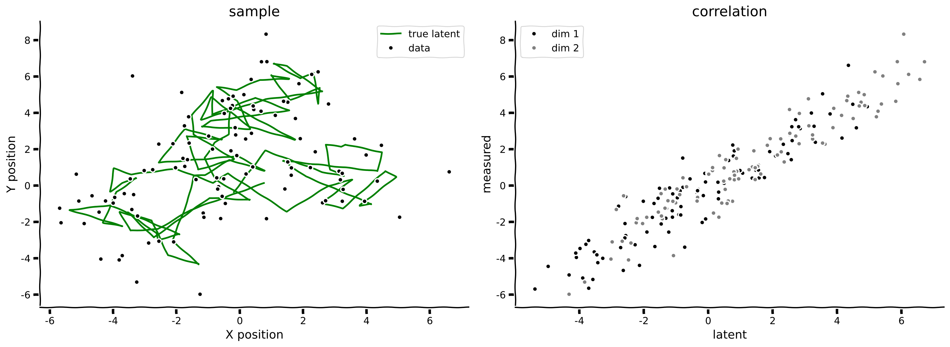
この演習では、線形動的システムの動力学関数を実装し、潜在空間の軌跡（上記パラメータセットに基づく）とノイズを含む測定値の両方をサンプリングします。

def sample_lds(n_timesteps, params, seed=0):
  """ Generate samples from a Linear Dynamical System specified by the provided
  parameters.

  Args:
  n_timesteps (int): the number of time steps to simulate
  params (dict): a dictionary of model parameters: (D, Q, H, R, mu_0, sigma_0)
  seed (int): a random seed to use for reproducibility checks

  Returns:
  ndarray, ndarray: the generated state and observation data
  """
  n_dim_state = params['D'].shape[0]
  n_dim_obs = params['H'].shape[0]

  # set seed
  np.random.seed(seed)

  # precompute random samples from the provided covariance matrices
  # mean defaults to 0
  mi = stats.multivariate_normal(cov=params['Q']).rvs(n_timesteps)
  eta = stats.multivariate_normal(cov=params['R']).rvs(n_timesteps)

  # initialize state and observation arrays
  state = np.zeros((n_timesteps, n_dim_state))
  obs = np.zeros((n_timesteps, n_dim_obs))

  ###################################################################
  ## TODO for students: compute the next state and observation values
  # Fill out function and remove
  raise NotImplementedError("Student exercise: compute the next state and observation values")
  ###################################################################

  # simulate the system
  for t in range(n_timesteps):
    # write the expressions for computing state values given the time step
    if t == 0:
      state[t] = ...
    else:
      state[t] = ...

    # write the expression for computing the observation
    obs[t] = ...

  return state, obs


state, obs = sample_lds(100, params)
print('sample at t=3 ', state[3])
plot_kalman(state, obs, title='sample')

解答を見る$

出力例:

# @title Submit your feedback
content_review(f"{feedback_prefix}_Sampling_from_a_linear_dynamical_system_Exercise")

インタラクティブデモ 1: システムダイナミクスの調整

線形動的システムのパラメータの理解を試すために、以下の変更を行った場合に何が起こるか考えてみましょう：

1. 観測ノイズ $R$ を減らす
2. それぞれの時間的ダイナミクス $D$ を増やす

以下のインタラクティブウィジェットを使って、$R$ と $D$ の値を変化させてみてください。

# @markdown Make sure you execute this cell to enable the widget!

@widgets.interact(R=widgets.FloatLogSlider(1., min=-2, max=2),
                  D=widgets.FloatSlider(0.9, min=0.0, max=1.0, step=.01))
def explore_dynamics(R=0.1, D=0.5):
  params = {
  'D': D * np.eye(n_dim_state),  # state transition matrix
  'Q': np.eye(n_dim_obs),  # state noise covariance
  'H': np.eye(n_dim_state),  # observation matrix
  'R': R * np.eye(n_dim_obs),  # observation noise covariance
  'mu_0': np.zeros(n_dim_state),  # initial state mean,
  'sigma_0': 0.1 * np.eye(n_dim_state),  # initial state noise covariance
  }

  state, obs = sample_lds(100, params)
  plot_kalman(state, obs, title='sample')

# @title Submit your feedback
content_review(f"{feedback_prefix}_Adjusting_System_Dynamics_Interactive_Demo")

セクション 2: カルマンフィルタリング

#@title Video 3: Kalman Filtering
# Insert the ID of the corresponding youtube video
from IPython.display import YouTubeVideo
video = YouTubeVideo(id="VboZOV9QMOI", width=854, height=480, fs=1)
print("Video available at https://youtu.be/" + video.id)
video

# @title Submit your feedback
content_review(f"{feedback_prefix}_Kalman_filtering_Video")

潜在状態変数 $s_t$ を、測定（観測）変数 $m_t$ から推定したい。

まず、$t=0,....T$ までフィルタリングを実行して潜在状態の推定値を得る。

ここで、$\hat{\mu}_t^{\rm pred}$ と $\hat{\Sigma}_t^{\rm pred}$ は以下のように導出される：

\begin{eqnarray}
$\hat{\mu}_1^{\rm pred}$ & = & D$\hat{\mu}_{0}$ \
$\hat{\mu}_t^{\rm pred}$ & = & D\hat{\mu}_{t-1} \end{eqnarray}

これは、$s_{t-1}$ の期待値を取り、遷移行列 $D$ を使って1ステップ先に予測した $s_t$ の予測値である。
共分散についても同様に、ノイズ共分散 $Q$ と、変数を $D$ でスケーリングすると共分散 $\Sigma$ が $D\Sigma D^\mathsf{T}$ でスケーリングされることを考慮して計算する：

\begin{eqnarray}
$\hat{\Sigma}_0^{\rm pred}$ & = & D$\hat{\Sigma}_{0}D^\mathsf{T}+Q$ \
$\hat{\Sigma}_t^{\rm pred}$ & = & D\hat{\Sigma}_{t-1}D^\mathsf{T}+Q \end{eqnarray}

次に、最新の観測値からベイズ更新を行い、$\hat{\mu}_t^{\rm filter}$ と $\hat{\Sigma}_t^{\rm filter}$ を得る。

予測を観測空間に射影する：

実際のデータで予測を更新する：

\begin{eqnarray}
s_t^{\rm filter} & $\sim$ & $\mathcal{N}(\hat{\mu}_t^{\rm filter}, \hat{\Sigma}_t^{\rm filter})$ \
$\hat{\mu}_t^{\rm filter}$ & = & $\hat{\mu}_t^{\rm pred}+K_t(m_t-H\hat{\mu}_t^{\rm pred})$ \
$\hat{\Sigma}_t^{\rm filter}$ & = & ($I-K_tH)$\hat{\Sigma}_t^{\rm pred} \end{eqnarray}

カルマンゲイン行列：

潜在状態のみの予測を観測空間に射影し、予測とデータの誤差 $m_t-HDz_{t-1}$ に比例した補正を計算する。この補正の係数がカルマンゲイン行列である。

解釈

もし測定ノイズが小さく、ダイナミクスが速ければ、推定は主に現在観測されたデータに依存する。
測定ノイズが大きい場合、カルマンフィルタは過去の観測も利用し、基礎となる状態がある程度予測可能であればそれらを組み合わせる。

フィルタリングの影響を探るために、以下のノイズのある振動系を使う。

# task dimensions
n_dim_state = 2
n_dim_obs = 2
T = 100

# initialize model parameters
params = {
  'D': np.array([[1., 1.], [-(2*np.pi/20.)**2., .9]]),  # state transition matrix
  'Q': np.eye(n_dim_obs),                               # state noise covariance
  'H': np.eye(n_dim_state),                             # observation matrix
  'R': 100.0 * np.eye(n_dim_obs),                       # observation noise covariance
  'mu_0': np.zeros(n_dim_state),                        # initial state mean
  'sigma_0': 0.1 * np.eye(n_dim_state),                 # initial state noise covariance
}

state, obs = sample_lds(T, params)
plot_kalman(state, obs, title='Sample')

コーディング演習 2: カルマンフィルタの実装

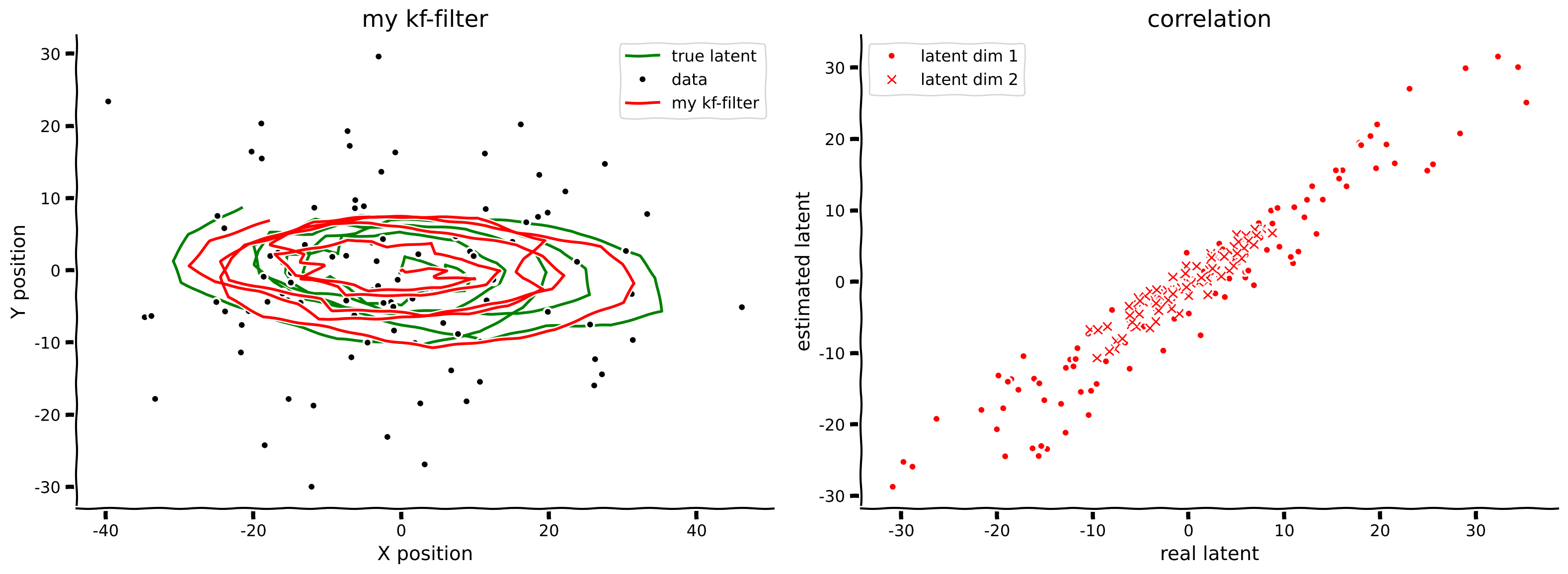
この演習ではカルマンフィルタ（順方向）プロセスを実装する。焦点は各時刻でのカルマンゲイン、フィルタ平均、フィルタ共分散の式を書くことにある（上記の式を参照）。

def kalman_filter(data, params):
  """ Perform Kalman filtering (forward pass) on the data given the provided
  system parameters.

  Args:
    data (ndarray): a sequence of observations of shape(n_timesteps, n_dim_obs)
    params (dict): a dictionary of model parameters: (D, Q, H, R, mu_0, sigma_0)

  Returns:
    ndarray, ndarray: the filtered system means and noise covariance values
  """
  # pulled out of the params dict for convenience
  D = params['D']
  Q = params['Q']
  H = params['H']
  R = params['R']

  n_dim_state = D.shape[0]
  n_dim_obs = H.shape[0]
  I = np.eye(n_dim_state)  # identity matrix

  # state tracking arrays
  mu = np.zeros((len(data), n_dim_state))
  sigma = np.zeros((len(data), n_dim_state, n_dim_state))

  # filter the data
  for t, y in enumerate(data):
    if t == 0:
      mu_pred = params['mu_0']
      sigma_pred = params['sigma_0']
    else:
      mu_pred = D @ mu[t-1]
      sigma_pred = D @ sigma[t-1] @ D.T + Q

    ###########################################################################
    ## TODO for students: compute the filtered state mean and covariance values
    # Fill out function and remove
    raise NotImplementedError("Student exercise: compute the filtered state mean and covariance values")
    ###########################################################################
    # write the expression for computing the Kalman gain
    K = ...
    # write the expression for computing the filtered state mean
    mu[t] = ...
    # write the expression for computing the filtered state noise covariance
    sigma[t] = ...

  return mu, sigma


filtered_state_means, filtered_state_covariances = kalman_filter(obs, params)
plot_kalman(state, obs, filtered_state_means, title="my kf-filter",
            color='r', label='my kf-filter')

解答を見る$

出力例:

# @title Submit your feedback
content_review(f"{feedback_prefix}_Implement_Kalman_filtering_Exercise")

セクション 3: 眼球注視データのフィッティング

#@title Video 4: Fitting Eye Gaze Data
# Insert the ID of the corresponding youtube video
from IPython.display import YouTubeVideo
video = YouTubeVideo(id="M7OuXmVWHGI", width=854, height=480, fs=1)
print("Video available at https://youtu.be/" + video.id)
video

# @title Submit your feedback
content_review(f"{feedback_prefix}_Fitting_Eye_Gaze_Data_Video")

眼球注視の追跡は実験やユーザーインターフェースの両方で使われる。画面上のどこをピクセル座標で見ているかを正確に推定することは、これらの測定に内在する様々なノイズ源のために難しい。
主なノイズ源は、眼球追跡装置自体の一般的な精度と、時間経過によるキャリブレーションの維持度合いである。周囲の光の変化や被験者の位置変化もセンサーの精度を低下させる。まばたきはデータストリームの中断という別のノイズ形態をもたらし、これも対処が必要である。

幸いにも、先ほど学んだカルマンフィルタはノイズのある眼球注視データを扱うための候補解となる。ここでは、MIT Eyetracking Database [Judd et al. 2009] から取得した小さなデータセットにこれらの手法を適用する方法を見ていく。このデータは視覚的顕著性$のモデル化の一環として収集されたものである。すなわち、画像が与えられたとき、人が最も注視しそうな場所を予測できるかを調べるためのものである。

# load eyetracking data
subjects, images = load_eyetracking_data()

インタラクティブデモ 2: 目の視線追跡

3つの刺激画像と5人の異なる被験者の視線データがあります。各被験者は画像が表示される前に画面中央を注視し、その後数秒間自由に見回しました。以下のウィジェットを使って、異なる被験者が提示された画像をどのように視覚的にスキャンしたかを見ることができます。被験者IDを-1にすると、視線の軌跡なしで刺激画像のみが表示されます。

画像は表示のために下記でリスケールされていますが、タスク中は元のアスペクト比のままでした。

# @markdown Make sure you execute this cell to enable the widget!

@widgets.interact(subject_id=widgets.IntSlider(-1, min=-1, max=4),
                  image_id=widgets.IntSlider(0, min=0, max=2))
def plot_subject_trace(subject_id=-1, image_id=0):
  if subject_id == -1:
    subject = np.zeros((3, 0, 2))
  else:
    subject = subjects[subject_id]
  data = subject[image_id]
  img = images[image_id]

  fig, ax = plt.subplots()
  ax.imshow(img, aspect='auto')
  ax.scatter(data[:, 0], data[:, 1], c='m', s=100, alpha=0.7)
  ax.set(xlim=(0, img.shape[1]), ylim=(img.shape[0], 0))
  plt.show(fig)

# @title Submit your feedback
content_review(f"{feedback_prefix}_Tracking_Eye_Gaze_Interactive_Demo")

セクション 3.1: pykalmanによるデータフィッティング

データが揃ったので、カルマンフィルタを使って真の視線のより良い推定を行いたいと思います。ここまではLDSのパラメータを知っていましたが、ここではデータから直接パラメータを推定する必要があります。EMアルゴリズムを用いた推定を扱うために、pykalmanパッケージを使用します。EMアルゴリズムはボーナスマテリアルで簡単に説明した、有用で影響力のある学習アルゴリズムです。

pykalmanでモデルをフィットさせる前に、ライブラリで使われている命名規則をいくつか紹介します：

\begin{align}
D &: \texttt{transition_matrices} &
Q &: \texttt{transition_covariance} \
H &: \texttt{observation_matrices} &
R &: \texttt{observation_covariance} \
$\mu_0$ &: \texttt{initial_state_mean} & $\Sigma_0$ &: \texttt{initial_state_covariance} \end{align}

まず最初に、潜在状態の次元数の推測を提供する必要があります。ここでは、動的モデルが観測データ（ピクセルのx,y座標）と直接対応していると仮定し、状態次元を2とします。

また、EMアルゴリズムにどのパラメータをフィットさせるか決める必要があります。今回は、EMアルゴリズムに動的パラメータ、すなわち$D$, $Q$, $H$, $R$の行列を推定させます。

以下のコードでこれらの設定を使ってpykalmanのKalmanFilterオブジェクトをセットアップします。

# set up our KalmanFilter object and tell it which parameters we want to
# estimate
np.random.seed(1)

n_dim_obs = 2
n_dim_state = 2

kf = pykalman.KalmanFilter(
  n_dim_state=n_dim_state,
  n_dim_obs=n_dim_obs,
  em_vars=['transition_matrices', 'transition_covariance',
           'observation_matrices', 'observation_covariance']
)

実験デザインの報告から、被験者は画像が表示される直前に画面中央を注視していたことがわかっているため、初期状態推定$\mu_0$を刺激画像の中央ピクセル（このサンプルデータセットの最初のデータ点）に設定し、対応する低い初期ノイズ共分散$\Sigma_0$を設定します。すべて準備が整ったら、データにフィットさせる段階です。

# Choose a subject and stimulus image
subject_id = 1
image_id = 2
data = subjects[subject_id][image_id]

# Provide the initial states
kf.initial_state_mean = data[0]
kf.initial_state_covariance = 0.1*np.eye(n_dim_state)

# Estimate the parameters from data using the EM algorithm
kf.em(data)

print(f'D=\n{kf.transition_matrices}')
print(f'Q =\n{kf.transition_covariance}')
print(f'H =\n{kf.observation_matrices}')
print(f'R =\n{kf.observation_covariance}')

EMアルゴリズムが様々な動的パラメータのフィットを見つけたことがわかります。注目すべき点は、状態行列と観測行列の両方がほぼ単位行列に近いことで、これはx座標とy座標の動的が互いに独立であり、主にノイズ共分散の影響を受けていることを意味します。

このモデルを使って被験者の観測データを平滑化できます。元の画像に加え、このモデルが同じ被験者の他の画像で記録された視線や、異なる被験者の視線に対してもどのように機能するかを見ることができます。

以下に、3つの刺激画像に記録された視線をマゼンタで、フィルタからの平滑化された状態を緑で重ねて示しています。視線開始点はオレンジの三角形、視線終了点はオレンジの四角形でマークしています。

# @markdown Make sure you execute this cell to enable the widget!

@widgets.interact(subject_id=widgets.IntSlider(1, min=0, max=4))
def plot_smoothed_traces(subject_id=0):
  subject = subjects[subject_id]
  fig, axes = plt.subplots(ncols=3, figsize=(18, 4))
  for data, img, ax in zip(subject, images, axes):
    ax = plot_gaze_data(data, img=img, ax=ax)
    plot_kf_state(kf, data, ax, show=False)
  plt.show()

# @title Submit your feedback
content_review(f"{feedback_prefix}_DaySummary")

議論の質問

1. なぜ1人の被験者のトレースだけで全被験者に対して十分なフィットが得られたと思いますか？もしEMでデータをフィットさせる際にsubjec$t_id$やimag$e_id$を変更したら、フィットは異なると思いますか？

2. 目は正確に線形動的システムに従っているわけではないと考えられます。それでもこの演習ではカルマンフィルタを適用しました。この不一致にもかかわらず、これらのアルゴリズムはよく機能します。真のプロセスと仮定したプロセスの間でどのような違いがあるか議論してください。これらの違いによって起こりうる誤りは何でしょうか？

3. 最後に、元のタスクはこのデータを使って視覚的顕著性のモデルを開発することでした。カルマンフィルタは観測された視線データの平滑な推定を提供できますが、なぜ視線が特定の方向に向かうのかについては何も教えてくれません。実際、パラメータからデータをサンプリングしてプロットすると、ランダムウォークのような結果になります。

kf_state, kf_data = kf.sample(len(data))
ax = plot_gaze_data(kf_data, img=images[2])
plot_kf_state(kf, kf_data, ax)

これは驚くべきことではありません。なぜなら、モデルには視線が検出されたピクセル以外の観測データを与えていないからです。次にどこを見るかという潜在状態を決定する要因は、単に前回の注視位置だけではないと考えられます。

まとめると、カルマンフィルターは視線軌跡自体を平滑化するには良い選択肢であり、特に低品質のアイ・トラッカーを使う場合やノイズの多い環境条件下では有効ですが、線形動的システムは視覚的顕著性をモデル化するというはるかに難しい課題に対しては適切なアプローチではないかもしれません。

まばたきの処理

MITアイ・トラッキングデータベースでは、生の追跡データに被験者のまばたき時刻が含まれています。これはデータストリーム内で負のピクセル座標値として表現されています。

これらのサンプルを単純にストリームから削除して対処することもできますが、これには別の問題が生じます。例えば、各サンプルが固定のタイムステップに対応している場合に、任意にサンプルを削除すると、サンプル間の一貫したタイムステップの整合性が失われます。時系列データでは、データが存在しなかったことにするよりも、欠損としてフラグを立てるほうが望ましい場合があります。

もう一つの解決策はマスク付き配列を使うことです。numpyのマスク付き配列は、どの要素をマスクすべきかを示すブール型のマスク配列を埋め込んだndarrayです。配列に対して計算を行う際、マスクされた要素は無視されます。matplotlibやpykalmanはマスク付き配列に対応しており、実際このノートブックで扱うデータもこの方法で処理されています。

このノートブック用のデータセットを準備する際、元のデータセットはすべての視線データをマスク付き配列として前処理し、$x$または$y$座標が負のピクセルに対してマスクを有効にしています。

ボーナス

ガウス分布の結合分布、周辺分布、条件付き分布の復習

\begin{eqnarray}
z & = & \begin{bmatrix}x $\y\end{bmatrix}\sim N\left(\begin{bmatrix}a$ $\b\end{bmatrix}, \begin{bmatrix}A$ & C $\C^\mathsf{T}$ & B\end{bmatrix}\right) \end{eqnarray}

このとき、周辺分布は

\begin{eqnarray}
x & $\sim$ & $\mathcal{N}(a, A)$ \
y & $\sim$ & \mathcal{N}(b,B) \end{eqnarray}

条件付き分布は次のようになります。

\begin{eqnarray}
x|y & $\sim$ & $\mathcal{N}(a+CB^{-1}(y-b), A-CB^{-1}C^\mathsf{T})$ \
y|x & $\sim$ & $\mathcal{N}(b+C^\mathsf{T} A^{-1}(x-a), B-C^\mathsf{T} A^{-1}C)
\end{eqnarray}

$重要なポイント: 共分散ガウス分布が与えられたとき、条件付き分布を導出できる

カルマン平滑化

#@title Video 5: Kalman Smoothing and the EM Algorithm
# Insert the ID of the corresponding youtube video
from IPython.display import YouTubeVideo
video = YouTubeVideo(id="4Ar2mYz1Nms", width=854, height=480, fs=1)
print("Video available at https://youtu.be/" + video.id)
video

# @title Submit your feedback
content_review(f"{feedback_prefix}_Kalman_Smoothing_and_the_EM_Algorithm_Bonus_Video")

$y_T$ から $y_0$ へ、順方向の計算結果（$\hat{\mu}_t^{\rm filter}, \hat{\Sigma}_t^{\rm filter}, P_t=\hat{\Sigma}_{t+1}^{\rm pred}$）を用いて逆方向に伝播させることで推定値を得ます。

\begin{eqnarray}
$s_t$ & $\sim$ & $\mathcal{N}(\hat{\mu}_t^{\rm smooth}, \hat{\Sigma}_t^{\rm smooth})$ \
$\hat{\mu}_t^{\rm smooth}$ & = & $\hat{\mu}_t^{\rm filter}+J_t(\hat{\mu}_{t+1}^{\rm smooth}-D\hat{\mu}_t^{\rm filter})$ \
$\hat{\Sigma}_t^{\rm smooth}$ & = & $\hat{\Sigma}_t^{\rm filter}+J_t(\hat{\Sigma}_{t+1}^{\rm smooth}-P_t)J_t^\mathsf{T}$ \
$J_t$ & = & \hat{\Sigma}_t^{\rm filter}D^\mathsf{T} P_t^{-1} \end{eqnarray}

これにより、$z_t$ の最終的な推定値が得られます。

\begin{eqnarray}
$\hat{\mu}_t$ & = & $\hat{\mu}_t^{\rm smooth}$ \
$\hat{\Sigma}_t$ & = & \hat{\Sigma}_t^{\rm smooth} \end{eqnarray}

ボーナスコーディング演習 3: カルマン平滑化の実装

この演習では、カルマン平滑化（後ろ向き）プロセスを実装します。再び、平滑化された平均、平滑化された共分散、および $J_t$ の値を計算する式の記述に焦点を当てます。

def kalman_smooth(data, params):
  """ Perform Kalman smoothing (backward pass) on the data given the provided
  system parameters.

  Args:
    data (ndarray): a sequence of observations of shape(n_timesteps, n_dim_obs)
    params (dict): a dictionary of model parameters: (D, Q, H, R, mu_0, sigma_0)

  Returns:
    ndarray, ndarray: the smoothed system means and noise covariance values
  """
  # pulled out of the params dict for convenience
  D= params['D']
  Q = params['Q']
  H = params['H']
  R = params['R']

  n_dim_state = D.shape[0]
  n_dim_obs = H.shape[0]

  # first run the forward pass to get the filtered means and covariances
  mu, sigma = kalman_filter(data, params)

  # initialize state mean and covariance estimates
  mu_hat = np.zeros_like(mu)
  sigma_hat = np.zeros_like(sigma)
  mu_hat[-1] = mu[-1]
  sigma_hat[-1] = sigma[-1]

  # smooth the data
  for t in reversed(range(len(data)-1)):
    sigma_pred = D@ sigma[t] @ D.T + Q  # sigma_pred at t+1
    ###########################################################################
    ## TODO for students: compute the smoothed state mean and covariance values
    # Fill out function and remove
    raise NotImplementedError("Student exercise: compute the smoothed state mean and covariance values")
    ###########################################################################

    # write the expression to compute the Kalman gain for the backward process
    J = ...
    # write the expression to compute the smoothed state mean estimate
    mu_hat[t] = ...
    # write the expression to compute the smoothed state noise covariance estimate
    sigma_hat[t] = ...

  return mu_hat, sigma_hat


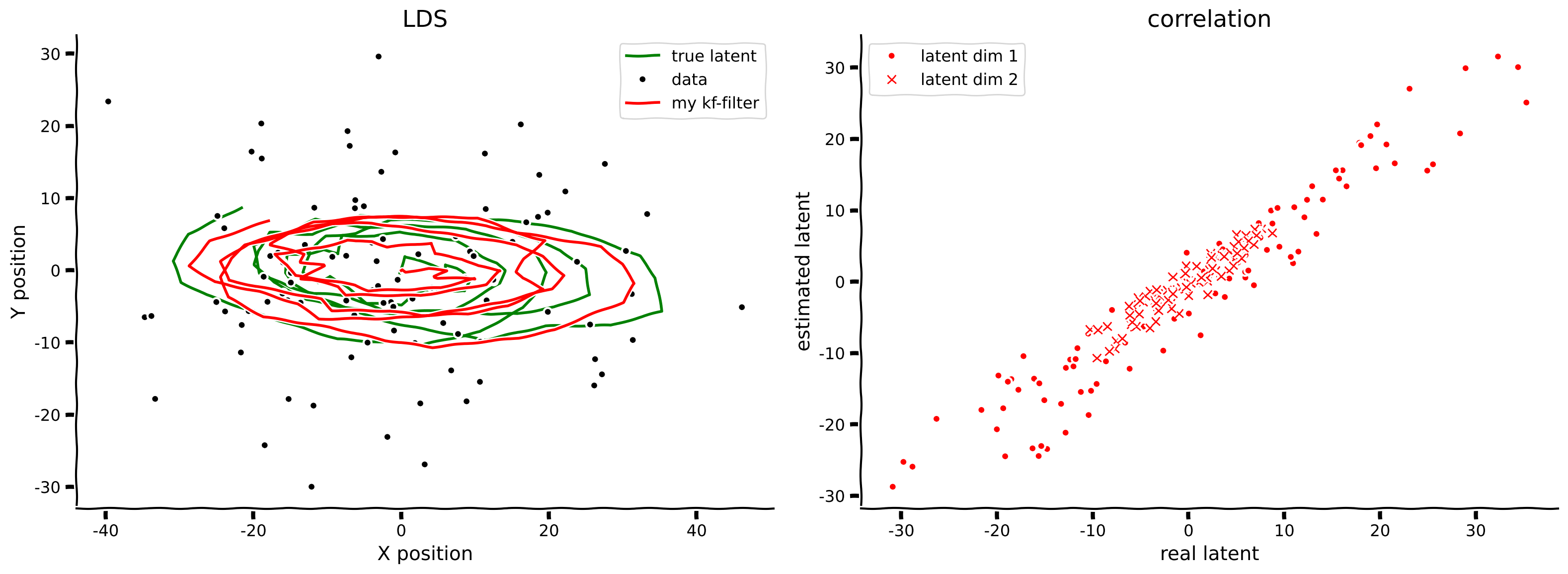
smoothed_state_means, smoothed_state_covariances = kalman_smooth(obs, params)
axes = plot_kalman(state, obs, filtered_state_means, color="r",
                   label="my kf-filter")
plot_kalman(state, obs, smoothed_state_means, color="b",
            label="my kf-smoothed", axes=axes)

解答を見る$

出力例:

# @title Submit your feedback
content_review(f"{feedback_prefix}_Implement_Kalman_smoothing_Bonus_Exercise")

順方向フィルタリング vs 逆方向スムージング

両方の実装ができたので、フィルタリング（順方向）とスムージング（逆方向）による推定状態と真の潜在状態との間の平均二乗誤差（MSE）を計算して性能を比較してみましょう。

print(f"Filtered MSE: {np.mean((state - filtered_state_means)**2):.3f}")
print(f"Smoothed MSE: {np.mean((state - smoothed_state_means)**2):.3f}")

この例では、スムージングによる推定が明らかにフィルタリングより優れています。これは理にかなっています。なぜなら順方向パスは過去の測定値のみを使用しますが、逆方向パスは未来の測定値も利用できるため、収集したすべてのデータを考慮して順方向の推定を修正できるからです。

では、なぜスムージングを使わずにカルマンフィルタリングだけを使うのでしょうか？カルマンフィルタリングは既に観測されたデータ（つまり過去）にのみ依存するため、ストリーミングやオンラインの設定で実行可能です。一方、カルマンスムージングは未来のデータを利用するため、バッチ処理やオフラインの設定でしか適用できません。リアルタイムの補正が必要ならカルマンフィルタリングを使い、既に収集されたデータを扱うならカルマンスムージングを使いましょう。

このオンラインのケースは、通常脳が直面する状況です。

期待値最大化（EM）アルゴリズム

• $\log p(m|\theta)$ を最大化したい

• 潜在状態を周辺化する必要がある（これは解析的に扱いにくい）

• 潜在状態分布を近似する確率分布 $q(s)$ を導入する

• 次のように書き換えられる

• $\mathcal{L}(q,\theta)$ は $m$ と $s$ の結合分布を含む

• $KL(q||p)$ は $s|m$ の条件付き分布を含む

期待値ステップ（Eステップ）

• パラメータは固定
• 良い近似 $q(s)$ を見つける：$q(s)$ に関して下限 $\mathcal{L}(q,\theta)$ を最大化する
• （カルマンフィルタ＋スムーザーは既に実装済み）

最大化ステップ（Mステップ）

• 分布 $q(s)$ は固定
• パラメータを変えて下限 $\mathcal{L}(q,\theta)$ を最大化する

前述の通り、Eステップはカルマンフィルタとスムーザーで既に実質的に解決しています。Mステップはさらなる導出が必要で、付録で扱います。Mステップの実装は皆さんに任せず、代わりにEMを実装済みのライブラリを使って認知神経科学の実験データを探索してみましょう。

線形動的システム（LDS）のMステップ

（Bishop著、13.3.2節「LDSにおける学習」を参照）
確率分布のパラメータを更新する

Mステップの更新にはカルマンスムージングの結果から得られる以下の事後周辺分布が必要です：$\hat{\mu}_t^{\rm smooth}, \hat{\Sigma}_t^{\rm smooth}$

\begin{eqnarray}
$\mathbb{E}$[s_t] &=& $\hat{\mu}_t$ \
$\mathbb{E}$[s_ts_{t-1}^$\mathsf{T}$] &=& $J_{t-1}$$\hat{\Sigma}_t+\hat{\mu}_t\hat{\mu}_{t-1}^\mathsf{T}$\
$\mathbb{E}$[s_ts_{t}^$\mathsf{T}$] &=& $\hat{\Sigma}_t+\hat{\mu}t\hat{\mu}{t}^\mathsf{T}
\end{eqnarray}

$パラメータの更新

初期パラメータ

\begin{eqnarray}
$\mu_0^{\rm new}$&=& $\mathbb{E}$[s_0] \
Q_0^{\rm new} &=& $\mathbb{E}$[s_0s_0^$\mathsf{T}$]-$\mathbb{E}$[s_0]$\mathbb{E}$[s_0]^$\mathsf{T}$ \
\end{eqnarray}

隠れ（潜在）状態のパラメータ

\begin{eqnarray}
D^{\rm new} &=& \left(\sum_{t=2}^N \mathbb{E}[s_ts_{t-1}^\mathsf{T}]\right)\left(\sum_{t=2}^N \mathbb{E}[s_{t-1}s_{t-1}^$\mathsf{T}$]\right)^{-1} \
Q^{\rm new} &=& \frac{1}{T-1} \sum_{t=2}^N \mathbb{E}\big[s_ts_t^\mathsf{T} \big] - D^{\rm new}\mathbb{E}\big[s_{t-1}s_{t}^\mathsf{T} \big] - \mathbb{E}\big[s_ts_{t-1}^\mathsf{T} \big] D^{\rm new} + D^{\rm new}\mathbb{E}\big[s_{t-1}s_{t-1}^\mathsf{T} \big]$\big(D^{\rm new}\big)^\mathsf{T}
\end{eqnarray}

$

観測（測定）空間のパラメータ

\begin{eqnarray}
H^{\rm new} &=& \left(\sum_{t=1}^N y_t \mathbb{E}[s_t]^\mathsf{T}\right)\left(\sum_{t=1}^N \mathbb{E}[$s_t$ s_t^$\mathsf{T}$]\right)^{-1}\
R^{\rm new} &=& $\frac{1}{T}\sum_{t=1}^N y_ty_t^\mathsf{T} - H^{\rm new}\mathbb{E}$[s_t]y_t^$\mathsf{T} - y_t \mathbb{E}$[s_t]^$\mathsf{T}H^{\rm new} + H^{\rm new}\mathbb{E}$[s_ts_t^$\mathsf{T}$]H^{\rm new}\end{eqnarray}