チュートリアル 2: 隠れマルコフモデル

第3週、第3日目: 隠れた動態

Neuromatch Academyによる

コンテンツ作成者: Yicheng Fei（ジェシー・ライブジーとザック・ピトコウの協力による）

コンテンツレビュアー: ジョン・バトラー、マット・クラウス、ミーナクシ・コスラ、スピロス・チャブリス、マイケル・ワスコム

制作編集者: エラ・バティ、ガガナ・B、スピロス・チャブリス

チュートリアルの目的

チュートリアルの推定所要時間: 1時間5分

私たちの周りの世界はしばしば変化していますが、私たちが得られるのはノイズの多い感覚的な測定値だけです。同様に、神経系は離散的な状態（例：睡眠/覚醒）を切り替えますが、これは神経活動に与える影響を通じて間接的にしか観察できません。隠れマルコフモデル（HMM）は、測定値の時系列を用いてこれらの観測されていない（隠れたまたは潜在的な）状態について推論することを可能にします。

ここでは、HMMの遷移確率と測定ノイズを変化させることがデータにどのように影響するかを学びます。未来を予測するにつれて不確実性がどのように増加するか、そして測定からどのように情報を得るかを見ていきます。

私たちは、2つの状態の間をランダムに切り替わる2値の潜在変数 $s_t \in \{0,1\}$ と、現在の状態に関する証拠を提供する1次元ガウス放出モデル $m_t|s_t \sim \mathcal{N}(\mu_{s_t},\sigma^2_{s_t})$ を使用します。

このチュートリアルの終わりまでに、あなたは以下をできるようになるはずです：

隠れマルコフモデルにおける隠れ状態が時間とともにどのように変化するかを、言葉で、数学的に、コードで説明できる
隠れマルコフモデルにおける前向き推論を用いてデータから隠れ状態を推定できる
測定ノイズと状態遷移確率が未来の予測の不確実性や隠れ状態推定能力にどのように影響するかを説明できる

演習の概要

HMMからデータを生成する。
証拠なしでマルコフ連鎖における予測の伝播を計算する。
新しい証拠と過去の証拠からの予測を組み合わせて隠れ状態を推定する。

# @title Tutorial slides
# @markdown These are the slides for all videos in this tutorial.
from IPython.display import IFrame
link_id = "zsfbn"
print(f"If you want to download the slides: https://osf.io/download/{link_id}/")
IFrame(src=f"https://mfr.ca-1.osf.io/render?url=https://osf.io/{link_id}/?direct%26mode=render%26action=download%26mode=render", width=854, height=480)

セットアップ

# @title Install and import feedback gadget


from vibecheck import DatatopsContentReviewContainer
def content_review(notebook_section: str):
    return DatatopsContentReviewContainer(
        "",  # No text prompt
        notebook_section,
        {
            "url": "https://pmyvdlilci.execute-api.us-east-1.amazonaws.com/klab",
            "name": "neuromatch_cn",
            "user_key": "y1x3mpx5",
        },
    ).render()


feedback_prefix = "W3D2_T2"

# Imports
import numpy as np
import time
from scipy import stats
from scipy.optimize import linear_sum_assignment
from collections import namedtuple
import matplotlib.pyplot as plt
from matplotlib import patches

# @title Figure Settings
import logging
logging.getLogger('matplotlib.font_manager').disabled = True

import ipywidgets as widgets  # interactive display
from ipywidgets import interactive, interact, HBox, Layout,VBox
from IPython.display import HTML
%config InlineBackend.figure_format = 'retina'
plt.style.use("https://raw.githubusercontent.com/NeuromatchAcademy/course-content/NMA2020/nma.mplstyle")

# @title Plotting Functions

def plot_hmm1(model, states, measurements, flag_m=True):
  """Plots HMM states and measurements for 1d states and measurements.

  Args:
    model (hmmlearn model):               hmmlearn model used to get state means.
    states (numpy array of floats):       Samples of the states.
    measurements (numpy array of floats): Samples of the states.
  """
  T = states.shape[0]
  nsteps = states.size
  aspect_ratio = 2
  fig, ax1 = plt.subplots(figsize=(8,4))
  states_forplot = list(map(lambda s: model.means[s], states))
  ax1.step(np.arange(nstep), states_forplot, "-", where="mid", alpha=1.0, c="green")
  ax1.set_xlabel("Time")
  ax1.set_ylabel("Latent State", c="green")
  ax1.set_yticks([-1, 1])
  ax1.set_yticklabels(["-1", "+1"])
  ax1.set_xticks(np.arange(0,T,10))
  ymin = min(measurements)
  ymax = max(measurements)

  ax2 = ax1.twinx()
  ax2.set_ylabel("Measurements", c="crimson")

  # show measurement gaussian
  if flag_m:
    ax2.plot([T,T],ax2.get_ylim(), color="maroon", alpha=0.6)
    for i in range(model.n_components):
      mu = model.means[i]
      scale = np.sqrt(model.vars[i])
      rv = stats.norm(mu, scale)
      num_points = 50
      domain = np.linspace(mu-3*scale, mu+3*scale, num_points)

      left = np.repeat(float(T), num_points)
      # left = np.repeat(0.0, num_points)
      offset = rv.pdf(domain)
      offset *= T / 15
      lbl = "measurement" if i == 0 else ""
      # ax2.fill_betweenx(domain, left, left-offset, alpha=0.3, lw=2, color="maroon", label=lbl)
      ax2.fill_betweenx(domain, left+offset, left, alpha=0.3, lw=2, color="maroon", label=lbl)
      ax2.scatter(np.arange(nstep), measurements, c="crimson", s=4)
      ax2.legend(loc="upper left")
    ax1.set_ylim(ax2.get_ylim())
  plt.show(fig)


def plot_marginal_seq(predictive_probs, switch_prob):
  """Plots the sequence of marginal predictive distributions.

    Args:
      predictive_probs (list of numpy vectors): sequence of predictive probability vectors
      switch_prob (float):                      Probability of switching states.
  """
  T = len(predictive_probs)
  prob_neg = [p_vec[0] for p_vec in predictive_probs]
  prob_pos = [p_vec[1] for p_vec in predictive_probs]
  fig, ax = plt.subplots()
  ax.plot(np.arange(T), prob_neg, color="blue")
  ax.plot(np.arange(T), prob_pos, color="orange")
  ax.legend([
    "prob in state -1", "prob in state 1"
  ])
  ax.text(T/2, 0.05, "switching probability={}".format(switch_prob), fontsize=12,
          bbox=dict(boxstyle="round", facecolor="wheat", alpha=0.6))
  ax.set_xlabel("Time")
  ax.set_ylabel("Probability")
  ax.set_title("Forgetting curve in a changing world")
  plt.show(fig)


def plot_evidence_vs_noevidence(posterior_matrix, predictive_probs):
  """Plots the average posterior probabilities with evidence v.s. no evidence

  Args:
    posterior_matrix: (2d numpy array of floats): The posterior probabilities in state 1 from evidence (samples, time)
    predictive_probs (numpy array of floats):  Predictive probabilities in state 1 without evidence
  """
  nsample, T = posterior_matrix.shape
  posterior_mean = posterior_matrix.mean(axis=0)
  fig, ax = plt.subplots(1)
  ax.plot([0.0, T], [0., 0.], color="red", linestyle="dashed")
  ax.plot(np.arange(T), predictive_probs, c="orange", linewidth=2, label="No evidence")
  ax.scatter(np.tile(np.arange(T), (nsample, 1)), posterior_matrix, s=0.8,
             c="green", alpha=0.3, label="With evidence(Sample)")
  ax.plot(np.arange(T), posterior_mean, c='green',
          linewidth=2, label="With evidence(Average)")
  ax.legend()
  ax.set_yticks([0.0, 0.25, 0.5, 0.75, 1.0])
  ax.set_xlabel("Time")
  ax.set_ylabel("Probability in State +1")
  ax.set_title("Gain confidence with evidence")
  plt.show(fig)


def plot_forward_inference(model, states, measurements, states_inferred,
                           predictive_probs, likelihoods, posterior_probs,
                           t=None, flag_m=True, flag_d=True, flag_pre=True,
                           flag_like=True, flag_post=True):
  """Plot ground truth state sequence with noisy measurements, and ground truth states v.s. inferred ones

      Args:
          model (instance of hmmlearn.GaussianHMM): an instance of HMM
          states (numpy vector): vector of 0 or 1(int or Bool), the sequences of true latent states
          measurements (numpy vector of numpy vector): the un-flattened Gaussian measurements at each time point, element has size (1,)
          states_inferred (numpy vector): vector of 0 or 1(int or Bool), the sequences of inferred latent states
  """
  T = states.shape[0]
  if t is None:
    t = T-1
  nsteps = states.size
  fig, ax1 = plt.subplots(figsize=(11,6))
  # true states
  states_forplot = list(map(lambda s: model.means[s], states))
  ax1.step(np.arange(nstep)[:t+1], states_forplot[:t+1], "-", where="mid", alpha=1.0, c="green", label="true")
  ax1.step(np.arange(nstep)[t+1:], states_forplot[t+1:], "-", where="mid", alpha=0.3, c="green", label="")
  # Posterior curve
  delta = model.means[1] - model.means[0]
  states_interpolation = model.means[0] + delta * posterior_probs[:,1]
  if flag_post:
    ax1.step(np.arange(nstep)[:t+1], states_interpolation[:t+1], "-", where="mid", c="grey", label="posterior")

  ax1.set_xlabel("Time")
  ax1.set_ylabel("Latent State", c="green")
  ax1.set_yticks([-1, 1])
  ax1.set_yticklabels(["-1", "+1"])
  ax1.legend(bbox_to_anchor=(0,1.02,0.2,0.1), borderaxespad=0, ncol=2)

  ax2 = ax1.twinx()
  ax2.set_ylim(
      min(-1.2, np.min(measurements)),
      max(1.2, np.max(measurements))
      )
  if flag_d:
    ax2.scatter(np.arange(nstep)[:t+1], measurements[:t+1], c="crimson", s=4, label="measurement")
    ax2.set_ylabel("Measurements", c="crimson")

  # show measurement distributions
  if flag_m:
    for i in range(model.n_components):
      mu = model.means[i]
      scale = np.sqrt(model.vars[i])
      rv = stats.norm(mu, scale)
      num_points = 50
      domain = np.linspace(mu-3*scale, mu+3*scale, num_points)

      left = np.repeat(float(T), num_points)
      offset = rv.pdf(domain)
      offset *= T /15
      lbl = ""
      ax2.fill_betweenx(domain, left+offset, left, alpha=0.3, lw=2, color="maroon", label=lbl)
  ymin, ymax = ax2.get_ylim()
  width = 0.1 * (ymax-ymin) / 2.0
  centers = [-1.0, 1.0]
  bar_scale = 15

  # Predictions
  data = predictive_probs
  if flag_pre:
    for i in range(model.n_components):
      domain = np.array([centers[i]-1.5*width, centers[i]-0.5*width])
      left = np.array([t,t])
      offset = np.array([data[t,i]]*2)
      offset *= bar_scale
      lbl = "todays prior" if i == 0 else ""
      ax2.fill_betweenx(domain, left+offset, left, alpha=0.3, lw=2, color="dodgerblue", label=lbl)

  # Likelihoods
  data = likelihoods
  data /= np.sum(data,axis=-1, keepdims=True)
  if flag_like:
    for i in range(model.n_components):
      domain = np.array([centers[i]+0.5*width, centers[i]+1.5*width])
      left = np.array([t,t])
      offset = np.array([data[t,i]]*2)
      offset *= bar_scale
      lbl = "likelihood" if i == 0 else ""
      ax2.fill_betweenx(domain, left+offset, left, alpha=0.3, lw=2, color="crimson", label=lbl)
  # Posteriors
  data = posterior_probs
  if flag_post:
    for i in range(model.n_components):
      domain = np.array([centers[i]-0.5*width, centers[i]+0.5*width])
      left = np.array([t,t])
      offset = np.array([data[t,i]]*2)
      offset *= bar_scale
      lbl = "posterior" if i == 0 else ""
      ax2.fill_betweenx(domain, left+offset, left, alpha=0.3, lw=2, color="grey", label=lbl)
  if t<T-1:
    ax2.plot([t,t],ax2.get_ylim(), color='black',alpha=0.6)
  if flag_pre or flag_like or flag_post:
    ax2.plot([t,t],ax2.get_ylim(), color='black',alpha=0.6)

    ax2.legend(bbox_to_anchor=(0.4,1.02,0.6, 0.1), borderaxespad=0, ncol=4)
  ax1.set_ylim(ax2.get_ylim())
  return fig
  # plt.show(fig)

セクション0: はじめに

# @title Video 1: Introduction
from ipywidgets import widgets
from IPython.display import YouTubeVideo
from IPython.display import IFrame
from IPython.display import display


class PlayVideo(IFrame):
  def __init__(self, id, source, page=1, width=400, height=300, **kwargs):
    self.id = id
    if source == 'Bilibili':
      src = f'https://player.bilibili.com/player.html?bvid={id}&page={page}'
    elif source == 'Osf':
      src = f'https://mfr.ca-1.osf.io/render?url=https://osf.io/download/{id}/?direct%26mode=render'
    super(PlayVideo, self).__init__(src, width, height, **kwargs)


def display_videos(video_ids, W=400, H=300, fs=1):
  tab_contents = []
  for i, video_id in enumerate(video_ids):
    out = widgets.Output()
    with out:
      if video_ids[i][0] == 'Youtube':
        video = YouTubeVideo(id=video_ids[i][1], width=W,
                             height=H, fs=fs, rel=0)
        print(f'Video available at https://youtube.com/watch?v={video.id}')
      else:
        video = PlayVideo(id=video_ids[i][1], source=video_ids[i][0], width=W,
                          height=H, fs=fs, autoplay=False)
        if video_ids[i][0] == 'Bilibili':
          print(f'Video available at https://www.bilibili.com/video/{video.id}')
        elif video_ids[i][0] == 'Osf':
          print(f'Video available at https://osf.io/{video.id}')
      display(video)
    tab_contents.append(out)
  return tab_contents


video_ids = [('Youtube', 'pIXxVl1A4l0'), ('Bilibili', 'BV1Hh411r7JE')]
tab_contents = display_videos(video_ids, W=854, H=480)
tabs = widgets.Tab()
tabs.children = tab_contents
for i in range(len(tab_contents)):
  tabs.set_title(i, video_ids[i][0])
display(tabs)

# @title Submit your feedback
content_review(f"{feedback_prefix}_Introduction_Video")

セクション1: ガウス測定を伴う2値HMM

前回のチュートリアルとは異なり、HMMの潜在状態は固定されておらず、各時刻で異なる状態に切り替わる可能性があります。時間依存性は単純で、時刻 $t$ の状態の確率は完全に時刻 $t-1$ の状態によって決まります。これをマルコフ性と呼び、状態列全体 $\{s_1,...,s_t\}$ の依存関係はマルコフ連鎖と呼ばれる連鎖構造で表現されます。マルコフ連鎖は前提条件の統計学の日や線形システムチュートリアル2$で見たことがあります。

2値潜在動態のマルコフモデル

線形システムチュートリアル2$で見た2値スイッチング過程を再利用しましょう：状態は +1 または -1 のいずれかです。前の状態 $s_{t-1}=i$ から状態 $s_t=j$ に切り替わる確率は条件付き確率分布 $p(s_t = j| s_{t-1} = i)$ です。これらを $2\times 2$ の行列 $D$ （Dynamics）としてまとめます。

\begin{align}
D = $\begin{bmatrix}p(s_t$ = +1 | $s_{t-1}$ = +1) & $p(s_t$ = -1 | $s_{t-1}$ = +1)$\p(s_t = +1 | s_{t-1} = -1)$& $p(s_t$ = -1 | $s_{t-1}$ = -1)\end{bmatrix}
\end{align}

$D_{ij}$ は状態 $i$ から次の時刻で状態 $j$ に切り替わる遷移確率を表します。これはイントロや線形システムで使われている意味とは異なり（それらの遷移行列は我々のものの転置です）が、前提条件の統計学の日と整合しています。

現在の状態の確率は2次元ベクトルで表せます。

P_t = [p(s_t = +1), p(s_t = -1)]

この要素は現在の状態が +1 である確率と -1 である確率で、合計は1になります。

マルコフ過程に従い、時間とともに確率を更新します：

P_{t}= P_{t-1}D \tag{1}

状態が分かっている場合、 $P_{t-1}$ の要素は不確実性がないため1か0になります。

測定

_隠れマルコフモデル_では、潜在状態 $s_t$ を直接観測できません。代わりにノイズのある測定値 $m_t\sim p(m|s_t)$ を得ます。

# @title Video 2: Binary HMM with Gaussian measurements
from ipywidgets import widgets
from IPython.display import YouTubeVideo
from IPython.display import IFrame
from IPython.display import display


class PlayVideo(IFrame):
  def __init__(self, id, source, page=1, width=400, height=300, **kwargs):
    self.id = id
    if source == 'Bilibili':
      src = f'https://player.bilibili.com/player.html?bvid={id}&page={page}'
    elif source == 'Osf':
      src = f'https://mfr.ca-1.osf.io/render?url=https://osf.io/download/{id}/?direct%26mode=render'
    super(PlayVideo, self).__init__(src, width, height, **kwargs)


def display_videos(video_ids, W=400, H=300, fs=1):
  tab_contents = []
  for i, video_id in enumerate(video_ids):
    out = widgets.Output()
    with out:
      if video_ids[i][0] == 'Youtube':
        video = YouTubeVideo(id=video_ids[i][1], width=W,
                             height=H, fs=fs, rel=0)
        print(f'Video available at https://youtube.com/watch?v={video.id}')
      else:
        video = PlayVideo(id=video_ids[i][1], source=video_ids[i][0], width=W,
                          height=H, fs=fs, autoplay=False)
        if video_ids[i][0] == 'Bilibili':
          print(f'Video available at https://www.bilibili.com/video/{video.id}')
        elif video_ids[i][0] == 'Osf':
          print(f'Video available at https://osf.io/{video.id}')
      display(video)
    tab_contents.append(out)
  return tab_contents


video_ids = [('Youtube', 'z6KbKILMIPU'), ('Bilibili', 'BV1Sw41197Mj')]
tab_contents = display_videos(video_ids, W=854, H=480)
tabs = widgets.Tab()
tabs.children = tab_contents
for i in range(len(tab_contents)):
  tabs.set_title(i, video_ids[i][0])
display(tabs)

# @title Submit your feedback
content_review(f"{feedback_prefix}_Binary_HMM_with_Gaussian_measurements_Video")

コーディング演習 1.1: ガウス測定を伴う2値HMMのシミュレーション

この演習では、ガウス測定を伴う2値HMMを実装します。HMMは状態 +1 から開始し、状態間の遷移（ $-1 \rightarrow 1$ と $1 \rightarrow -1$ の両方）が確率 switch_prob で起こります。各状態は、状態 +1 なら平均 +1、状態 -1 なら平均 -1 のガウス分布から測定値を生成します。両状態の標準偏差は noise_level で与えられます。

次のセルの演習は3つのステップからなります：

ステップ1. create_HMM 内で遷移行列 transmat_（すなわち $D$ ）を完成させてください。

D = \begin{pmatrix} p_{\rm stay} & p_{\rm switch} \\ p_{\rm switch} & p_{\rm stay} \\ \end{pmatrix}

ここで $p_{\rm stay} = 1 - p_{\rm switch}$ です。

ステップ2. create_HMM 内でガウス測定 $m_t | s_t$ を指定してください。各状態の平均と標準偏差を設定します。

ステップ3. sample 内で遷移行列を用いて、前の状態 $s_{t-1}$ に基づく次の状態 $s_t$ の確率を指定してください。

この演習では、GaussianHMM1D という補助データ構造を使用します。これはHMMモデルの情報（状態の開始確率、遷移行列、ガウス分布の平均と分散、成分数）を設定し、簡単にアクセスできるようにしたものです。例えば、以下のようにモデルを設定できます：

  model = GaussianHMM1D(
    startprob = startprob_vec,
    transmat = transmat_mat,
    means = means_vec,
    vars = vars_vec,
    n_components = n_components
  )

そして分散は以下のようにアクセスできます：

model.vars

また、コード内では状態を -1 と +1 ではなく 0 と 1 として扱っていることに注意してください。

GaussianHMM1D = namedtuple('GaussianHMM1D', ['startprob', 'transmat','means','vars','n_components'])

def create_HMM(switch_prob=0.1, noise_level=1e-1, startprob=[1.0, 0.0]):
  """Create an HMM with binary state variable and 1D Gaussian measurements
  The probability to switch to the other state is `switch_prob`. Two
  measurement models have mean 1.0 and -1.0 respectively. `noise_level`
  specifies the standard deviation of the measurement models.

  Args:
      switch_prob (float): probability to jump to the other state
      noise_level (float): standard deviation of measurement models. Same for
      two components

  Returns:
      model (GaussianHMM instance): the described HMM
  """

  ############################################################################
  # Insert your code here to:
  #   * Create the transition matrix, `transmat_mat` so that the odds of
  #      switching is `switch_prob`
  #		* Set the measurement model variances, to `noise_level ^ 2` for both
  #      states
  raise NotImplementedError("`create_HMM` is incomplete")
  ############################################################################

  n_components = 2

  startprob_vec = np.asarray(startprob)

  # STEP 1: Transition probabilities
  transmat_mat = ... # np.array([[...], [...]])

  # STEP 2: Measurement probabilities

  # Mean measurements for each state
  means_vec = ...

  # Noise for each state
  vars_vec = np.ones(2) * ...

  # Initialize model
  model = GaussianHMM1D(
    startprob = startprob_vec,
    transmat = transmat_mat,
    means = means_vec,
    vars = vars_vec,
    n_components = n_components
  )

  return model


def sample(model, T):
  """Generate samples from the given HMM

  Args:
    model (GaussianHMM1D): the HMM with Gaussian measurement
    T (int): number of time steps to sample

  Returns:
    M (numpy vector): the series of measurements
    S (numpy vector): the series of latent states

  """
  ############################################################################
  # Insert your code here to:
  #   * take row i from `model.transmat` to get the transition probabilities
  #       from state i to all states
  raise NotImplementedError("`sample` is incomplete")
  ############################################################################
  # Initialize S and M
  S = np.zeros((T,),dtype=int)
  M = np.zeros((T,))

  # Calculate initial state
  S[0] = np.random.choice([0,1],p=model.startprob)

  # Latent state at time `t` depends on `t-1` and the corresponding transition probabilities to other states
  for t in range(1,T):

    # STEP 3: Get vector of probabilities for all possible `S[t]` given a particular `S[t-1]`
    transition_vector = ...

    # Calculate latent state at time `t`
    S[t] = np.random.choice([0,1],p=transition_vector)

  # Calculate measurements conditioned on the latent states
  # Since measurements are independent of each other given the latent states, we could calculate them as a batch
  means = model.means[S]
  scales = np.sqrt(model.vars[S])
  M = np.random.normal(loc=means, scale=scales, size=(T,))

  return M, S


# Set random seed
np.random.seed(101)

# Set parameters of HMM
T = 100
switch_prob = 0.1
noise_level = 2.0

# Create HMM
model = create_HMM(switch_prob=switch_prob, noise_level=noise_level)

# Sample from HMM
M, S = sample(model,T)
assert M.shape==(T,)
assert S.shape==(T,)

# Print values
print(M[:5])
print(S[:5])

最初の5つの測定値は以下のようになるはずです：

[-3.09355908 1.58552915 -3.93502804 -1.98819072 -1.32506947]

最初の5つの状態は以下の通りです：

[0 0 0 0 0]

解答を見る$

# @title Submit your feedback
content_review(f"{feedback_prefix}_Simulating_Binary_HMM_with_Gaussian_measurements_Exercise")

インタラクティブデモ 1.2: 2値HMM

以下のデモでは、類似のHMMをシミュレートしてプロットします。状態の切り替わる確率とノイズレベル（測定のガウス分布の標準偏差）を変更できます。空のボックスをクリックすると測定値も可視化できます。

まずは、以下の質問について考え、議論してください：

切り替わる確率が0の場合、状態はどうなるでしょうか？1の場合は？
ノイズが大きい場合と小さい場合、測定値はどのように見えるでしょうか？

その後、デモを操作して正しかったかどうか確かめてみましょう。

# @markdown Execute this cell to enable the widget!

nstep = 100

@widgets.interact
def plot_samples_widget(
    switch_prob=widgets.FloatSlider(min=0.0, max=1.0, step=0.02, value=0.1),
    log10_noise_level=widgets.FloatSlider(min=-1., max=1., step=.01, value=-0.3),
    flag_m=widgets.Checkbox(value=False, description='measurements',
                            disabled=False, indent=False)
    ):
  np.random.seed(101)
  model = create_HMM(switch_prob=switch_prob,
                     noise_level=10.**log10_noise_level)
  print(model)
  observations, states = sample(model, nstep)
  plot_hmm1(model, states, observations, flag_m=flag_m)

解答を見る$

# @title Submit your feedback
content_review(f"{feedback_prefix}_Binary_HMM_Interactive_Demo_and_Discussion")

# @title Video 3: Section 1 Exercises Discussion
from ipywidgets import widgets
from IPython.display import YouTubeVideo
from IPython.display import IFrame
from IPython.display import display


class PlayVideo(IFrame):
  def __init__(self, id, source, page=1, width=400, height=300, **kwargs):
    self.id = id
    if source == 'Bilibili':
      src = f'https://player.bilibili.com/player.html?bvid={id}&page={page}'
    elif source == 'Osf':
      src = f'https://mfr.ca-1.osf.io/render?url=https://osf.io/download/{id}/?direct%26mode=render'
    super(PlayVideo, self).__init__(src, width, height, **kwargs)


def display_videos(video_ids, W=400, H=300, fs=1):
  tab_contents = []
  for i, video_id in enumerate(video_ids):
    out = widgets.Output()
    with out:
      if video_ids[i][0] == 'Youtube':
        video = YouTubeVideo(id=video_ids[i][1], width=W,
                             height=H, fs=fs, rel=0)
        print(f'Video available at https://youtube.com/watch?v={video.id}')
      else:
        video = PlayVideo(id=video_ids[i][1], source=video_ids[i][0], width=W,
                          height=H, fs=fs, autoplay=False)
        if video_ids[i][0] == 'Bilibili':
          print(f'Video available at https://www.bilibili.com/video/{video.id}')
        elif video_ids[i][0] == 'Osf':
          print(f'Video available at https://osf.io/{video.id}')
      display(video)
    tab_contents.append(out)
  return tab_contents


video_ids = [('Youtube', 'bDDRgAvQeFA'), ('Bilibili', 'BV1dX4y1F7Fq')]
tab_contents = display_videos(video_ids, W=854, H=480)
tabs = widgets.Tab()
tabs.children = tab_contents
for i in range(len(tab_contents)):
  tabs.set_title(i, video_ids[i][0])
display(tabs)

# @title Submit your feedback
content_review(f"{feedback_prefix}_Section_1_Exercises_Discussion_Video")

応用例. 測定値は以下のようなものが考えられます：

魚群が左から右へ移動する際に異なる時間で捕獲される魚の数
イオンチャネルが開閉する際の膜電位
脳が睡眠状態間を移行する際のEEG周波数測定

これらのHMMでどのような現象をモデル化できそうか想像してみてください。

セクション2: HMMにおける未来の予測

チュートリアル開始からここまでの推定所要時間: 20分

# @title Video 4: Forgetting in a changing world
from ipywidgets import widgets
from IPython.display import YouTubeVideo
from IPython.display import IFrame
from IPython.display import display


class PlayVideo(IFrame):
  def __init__(self, id, source, page=1, width=400, height=300, **kwargs):
    self.id = id
    if source == 'Bilibili':
      src = f'https://player.bilibili.com/player.html?bvid={id}&page={page}'
    elif source == 'Osf':
      src = f'https://mfr.ca-1.osf.io/render?url=https://osf.io/download/{id}/?direct%26mode=render'
    super(PlayVideo, self).__init__(src, width, height, **kwargs)


def display_videos(video_ids, W=400, H=300, fs=1):
  tab_contents = []
  for i, video_id in enumerate(video_ids):
    out = widgets.Output()
    with out:
      if video_ids[i][0] == 'Youtube':
        video = YouTubeVideo(id=video_ids[i][1], width=W,
                             height=H, fs=fs, rel=0)
        print(f'Video available at https://youtube.com/watch?v={video.id}')
      else:
        video = PlayVideo(id=video_ids[i][1], source=video_ids[i][0], width=W,
                          height=H, fs=fs, autoplay=False)
        if video_ids[i][0] == 'Bilibili':
          print(f'Video available at https://www.bilibili.com/video/{video.id}')
        elif video_ids[i][0] == 'Osf':
          print(f'Video available at https://osf.io/{video.id}')
      display(video)
    tab_contents.append(out)
  return tab_contents


video_ids = [('Youtube', 'XOec560m61o'), ('Bilibili', 'BV1o64y1s7M7')]
tab_contents = display_videos(video_ids, W=854, H=480)
tabs = widgets.Tab()
tabs.children = tab_contents
for i in range(len(tab_contents)):
  tabs.set_title(i, video_ids[i][0])
display(tabs)

# @title Submit your feedback
content_review(f"{feedback_prefix}_Forgetting_in_a_changing_world_Video")

インタラクティブデモ 2.1: 変化する世界での忘却

たとえ現在の世界の状態が確実に分かっていても、世界は変化します。最後の測定から時間が経つにつれて、私たちの確信は徐々に薄れていきます。この演習では、測定なしで未来を予測する際に隠れマルコフモデルがどのように現在の状態を徐々に「忘れて」いくかを見ていきます。

初期状態が -1 であることが分かっていると仮定します。すなわち $s_0=-1$ で、 $p(s_0)=[1,0]$ です。時間に対する $p(s_t)$ をプロットします。

補助関数 simulate_prediction_only を調べ、予測分布が時間とともにどのように変化するか理解してください。
提供されたコードを使ってこの分布を時間軸でプロットし、スイッチング確率を制御するスライダーで過程の動態を操作してください。

スイッチング確率が低い場合と高い場合、どちらでより早く忘却しますか？なぜですか？prob_switch が $0.5$ を超えると曲線はどうなりますか？なぜでしょう？

# @markdown Execute this cell to enable helper function `simulate_prediction_only`

def simulate_prediction_only(model, nstep):
  """
  Simulate the diffusion of HMM with no observations

  Args:
    model (GaussianHMM1D instance): the HMM instance
    nstep (int): total number of time steps to simulate(include initial time)

  Returns:
    predictive_probs (list of numpy vector): the list of marginal probabilities
  """
  entropy_list = []
  predictive_probs = []
  prob = model.startprob
  for i in range(nstep):

    # Log probabilities
    predictive_probs.append(prob)

    # One step forward
    prob = prob @ model.transmat

  return predictive_probs

# @markdown Execute this cell to enable the widget!

np.random.seed(101)
T = 100
noise_level = 0.5

@widgets.interact(switch_prob=widgets.FloatSlider(min=0.0, max=1.0, step=0.01,
                                                  value=0.1))
def plot(switch_prob=switch_prob):
  model = create_HMM(switch_prob=switch_prob, noise_level=noise_level)
  predictive_probs = simulate_prediction_only(model, T)
  plot_marginal_seq(predictive_probs, switch_prob)

解答を見る$

# @title Submit your feedback
content_review(f"{feedback_prefix}_Forgetting_in_a_changing_world_Interactive_Demo_and_Discussion")

# @title Video 5: Section 2 Exercise Discussion
from ipywidgets import widgets
from IPython.display import YouTubeVideo
from IPython.display import IFrame
from IPython.display import display


class PlayVideo(IFrame):
  def __init__(self, id, source, page=1, width=400, height=300, **kwargs):
    self.id = id
    if source == 'Bilibili':
      src = f'https://player.bilibili.com/player.html?bvid={id}&page={page}'
    elif source == 'Osf':
      src = f'https://mfr.ca-1.osf.io/render?url=https://osf.io/download/{id}/?direct%26mode=render'
    super(PlayVideo, self).__init__(src, width, height, **kwargs)


def display_videos(video_ids, W=400, H=300, fs=1):
  tab_contents = []
  for i, video_id in enumerate(video_ids):
    out = widgets.Output()
    with out:
      if video_ids[i][0] == 'Youtube':
        video = YouTubeVideo(id=video_ids[i][1], width=W,
                             height=H, fs=fs, rel=0)
        print(f'Video available at https://youtube.com/watch?v={video.id}')
      else:
        video = PlayVideo(id=video_ids[i][1], source=video_ids[i][0], width=W,
                          height=H, fs=fs, autoplay=False)
        if video_ids[i][0] == 'Bilibili':
          print(f'Video available at https://www.bilibili.com/video/{video.id}')
        elif video_ids[i][0] == 'Osf':
          print(f'Video available at https://osf.io/{video.id}')
      display(video)
    tab_contents.append(out)
  return tab_contents


video_ids = [('Youtube', 'GRnlvxZ_ozk'), ('Bilibili', 'BV1DM4y1K7tK')]
tab_contents = display_videos(video_ids, W=854, H=480)
tabs = widgets.Tab()
tabs.children = tab_contents
for i in range(len(tab_contents)):
  tabs.set_title(i, video_ids[i][0])
display(tabs)

# @title Submit your feedback
content_review(f"{feedback_prefix}_Section_2_Exercise_Discussion_Video")

セクション3: HMMにおける前向き推論

チュートリアル開始からここまでの推定所要時間: 35分

# @title Video 6: Inference in an HMM
from ipywidgets import widgets
from IPython.display import YouTubeVideo
from IPython.display import IFrame
from IPython.display import display


class PlayVideo(IFrame):
  def __init__(self, id, source, page=1, width=400, height=300, **kwargs):
    self.id = id
    if source == 'Bilibili':
      src = f'https://player.bilibili.com/player.html?bvid={id}&page={page}'
    elif source == 'Osf':
      src = f'https://mfr.ca-1.osf.io/render?url=https://osf.io/download/{id}/?direct%26mode=render'
    super(PlayVideo, self).__init__(src, width, height, **kwargs)


def display_videos(video_ids, W=400, H=300, fs=1):
  tab_contents = []
  for i, video_id in enumerate(video_ids):
    out = widgets.Output()
    with out:
      if video_ids[i][0] == 'Youtube':
        video = YouTubeVideo(id=video_ids[i][1], width=W,
                             height=H, fs=fs, rel=0)
        print(f'Video available at https://youtube.com/watch?v={video.id}')
      else:
        video = PlayVideo(id=video_ids[i][1], source=video_ids[i][0], width=W,
                          height=H, fs=fs, autoplay=False)
        if video_ids[i][0] == 'Bilibili':
          print(f'Video available at https://www.bilibili.com/video/{video.id}')
        elif video_ids[i][0] == 'Osf':
          print(f'Video available at https://osf.io/{video.id}')
      display(video)
    tab_contents.append(out)
  return tab_contents


video_ids = [('Youtube', 'fErhvxE9SHs'), ('Bilibili', 'BV17f4y1571y')]
tab_contents = display_videos(video_ids, W=854, H=480)
tabs = widgets.Tab()
tabs.children = tab_contents
for i in range(len(tab_contents)):
  tabs.set_title(i, video_ids[i][0])
display(tabs)

# @title Submit your feedback
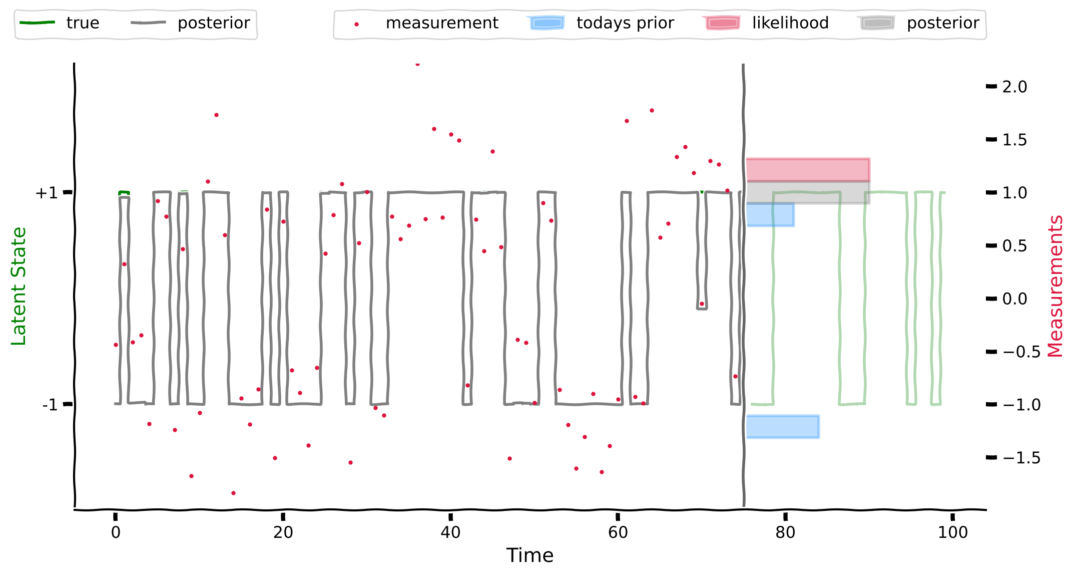
content_review(f"{feedback_prefix}_Forward_inference_in_an_HMM_Video")

コーディング演習 3.1: HMMの前向き推論

再帰的アルゴリズムとして、昨日の時刻 $t-1$ における事後分布 $p(s_{t-1}|m_{1:t-1})$ が既にあると仮定します。新しいデータ $m_{t}$ が入ると、アルゴリズムは以下のステップを実行します：

予測: 遷移行列 $D$ を用いて昨日の事後分布から今日の事前分布へ変換します：

\text{今日の事前分布}=p(s_t|m_{1:t-1})= p(s_{t-1}|m_{1:t-1}) D

更新: 測定 $m_t$ を取り入れて事後分布 $p(s_t|m_{0:t})$ を計算します。

\text{事後分布} \propto \text{事前分布}\cdot \text{尤度}=p(m_t|s_t)p(s_t|m_{0:t-1})

この演習では以下を行います：

ステップ1: 関数 markov_forward のコードを完成させ、次の時刻の予測周辺分布を計算する
ステップ2: 関数 one_step_update のコードを完成させ、予測確率とデータ尤度を組み合わせて新しい事後分布を計算する
- ヒント: 2つの可能な状態における $m_t$ の尤度を計算する関数 $compute_likelihood(model,M_t)$ を提供しています。
ステップ3: 提供されたコードを使って事後分布をプロットし、真の値と比較する

完全な前向き推論は simulate_forward_inference に実装されており、これは単に one_step_update を再帰的に呼び出しています。

# @markdown Execute to enable helper functions `compute_likelihood` and `simulate_forward_inference`

def compute_likelihood(model, M):
  """
  Calculate likelihood of seeing data `M` for all measurement models

  Args:
    model (GaussianHMM1D): HMM
    M (float or numpy vector)

  Returns:
    L (numpy vector or matrix): the likelihood
  """
  rv0 = stats.norm(model.means[0], np.sqrt(model.vars[0]))
  rv1 = stats.norm(model.means[1], np.sqrt(model.vars[1]))
  L = np.stack([rv0.pdf(M), rv1.pdf(M)],axis=0)
  if L.size==2:
    L = L.flatten()
  return L


def simulate_forward_inference(model, T, data=None):
  """
  Given HMM `model`, calculate posterior marginal predictions of x_t for T-1 time steps ahead based on
  evidence `data`. If `data` is not give, generate a sequence of measurements from first component.

  Args:
    model (GaussianHMM instance): the HMM
    T (int): length of returned array

  Returns:
    predictive_state1: predictive probabilities in first state w.r.t no evidence
    posterior_state1: posterior probabilities in first state w.r.t evidence
  """

  # First re-calculate hte predictive probabilities without evidence
  # predictive_probs = simulate_prediction_only(model, T)
  predictive_probs = np.zeros((T,2))
  likelihoods = np.zeros((T,2))
  posterior_probs = np.zeros((T, 2))
  # Generate an measurement trajectory conditioned on that latent state x is always 1
  if data is not None:
    M = data
  else:
    M = np.random.normal(model.means[0], np.sqrt(model.vars[0]), (T,))

  # Calculate marginal for each latent state x_t
  predictive_probs[0,:] = model.startprob
  likelihoods[0,:] = compute_likelihood(model, M[[0]])
  posterior = predictive_probs[0,:] * likelihoods[0,:]
  posterior /= np.sum(posterior)
  posterior_probs[0,:] = posterior

  for t in range(1, T):
    prediction, likelihood, posterior = one_step_update(model, posterior_probs[t-1], M[[t]])
    # normalize and add to the list
    posterior /= np.sum(posterior)
    predictive_probs[t,:] = prediction
    likelihoods[t,:] = likelihood
    posterior_probs[t,:] = posterior
  return predictive_probs, likelihoods, posterior_probs

help(compute_likelihood)
help(simulate_forward_inference)

def markov_forward(p0, D):
  """Calculate the forward predictive distribution in a discrete Markov chain

  Args:
    p0 (numpy vector): a discrete probability vector
    D (numpy matrix): the transition matrix, D[i,j] means the prob. to
    switch FROM i TO j

  Returns:
    p1 (numpy vector): the predictive probabilities in next time step
  """
  ##############################################################################
  # Insert your code here to:
  #    1. Calculate the predicted probabilities at next time step using the
  #      probabilities at current time and the transition matrix
  raise NotImplementedError("`markov_forward` is incomplete")
  ##############################################################################

  # Calculate predictive probabilities (prior)
  p1 = ...

  return p1

def one_step_update(model, posterior_tm1, M_t):
  """Given a HMM model, calculate the one-time-step updates to the posterior.
  Args:
    model (GaussianHMM1D instance): the HMM
    posterior_tm1 (numpy vector): Posterior at `t-1`
    M_t (numpy array): measurement at `t`

  Returns:
    posterior_t (numpy array): Posterior at `t`
  """
  ##############################################################################
  # Insert your code here to:
  #    1. Call function `markov_forward` to calculate the prior for next time
  #      step
  #    2. Calculate likelihood of seeing current data `M_t` under both states
  #      as a vector.
  #    3. Calculate the posterior which is proportional to
  #      likelihood x prediction elementwise,
  #    4. Don't forget to normalize
  raise NotImplementedError("`one_step_update` is incomplete")
  ##############################################################################

  # Calculate predictive probabilities (prior)
  prediction = markov_forward(...)

  # Get the likelihood
  likelihood = compute_likelihood(...)

  # Calculate posterior
  posterior_t = ...

  # Normalize
  posterior_t /= ...

  return prediction, likelihood, posterior_t


# Set random seed
np.random.seed(12)

# Set parameters
switch_prob = 0.4
noise_level = .4
t = 75

# Create and sample from model
model = create_HMM(switch_prob = switch_prob,
                    noise_level = noise_level,
                    startprob=[0.5, 0.5])

measurements, states = sample(model, nstep)

# Infer state sequence
predictive_probs, likelihoods, posterior_probs = simulate_forward_inference(model, nstep,
                                                            measurements)
states_inferred = np.asarray(posterior_probs[:,0] <= 0.5, dtype=int)

# Visualize
plot_forward_inference(
      model, states, measurements, states_inferred,
      predictive_probs, likelihoods, posterior_probs,t=t, flag_m = 0
    )

解答を見る$

出力例:

# @title Submit your feedback
content_review(f"{feedback_prefix}_Forward_inference_of_HMM_Exercise")

インタラクティブデモ 3.2: 2値HMMにおける前向き推論

今度は推論アルゴリズムを可視化します。スライダーやチェックボックスを操作して直感を養いましょう。

switch_prob と log10_noise_level のスライダーでスイッチング確率と測定ノイズレベルを変更できます。
t のスライダーで異なる時刻の予測（事前）確率、尤度、事後分布を表示できます。

推論が誤るのはどんな時でしょうか？例えば、switch_prob=0.1、log_10_noise_level=-0.2 に設定し、時刻 t=2 の確率を見てみてください。

# @markdown Execute this cell to enable the widget

nstep = 100

@widgets.interact
def plot_forward_inference_widget(
    switch_prob=widgets.FloatSlider(min=0.0, max=1.0, step=0.01, value=0.05),
    log10_noise_level=widgets.FloatSlider(min=-1., max=1., step=.01, value=0.1),
    t=widgets.IntSlider(min=0, max=nstep-1, step=1, value=nstep//2),
    flag_d=widgets.Checkbox(value=True, description='measurements',
                            disabled=False, indent=False),
    flag_pre=widgets.Checkbox(value=True, description='todays prior',
                              disabled=False, indent=False),
    flag_like=widgets.Checkbox(value=True, description='likelihood',
                               disabled=False, indent=False),
    flag_post=widgets.Checkbox(value=True, description='posterior',
                               disabled=False, indent=False),
    ):

  np.random.seed(102)

  # global model, measurements, states, states_inferred, predictive_probs, likelihoods, posterior_probs
  model = create_HMM(switch_prob=switch_prob,
                      noise_level=10.**log10_noise_level,
                      startprob=[0.5, 0.5])
  measurements, states = sample(model, nstep)

  # Infer state sequence
  predictive_probs, likelihoods, posterior_probs = simulate_forward_inference(model, nstep,
                                                              measurements)
  states_inferred = np.asarray(posterior_probs[:,0] <= 0.5, dtype=int)

  fig = plot_forward_inference(
        model, states, measurements, states_inferred,
        predictive_probs, likelihoods, posterior_probs,t=t,
        flag_m=0,
        flag_d=flag_d,flag_pre=flag_pre,flag_like=flag_like,flag_post=flag_post
      )
  plt.show(fig)

# @title Submit your feedback
content_review(f"{feedback_prefix}_Forward_inference_of_HMM_Interactive_Demo")

# @title Video 7: Section 3 Exercise Discussion
from ipywidgets import widgets
from IPython.display import YouTubeVideo
from IPython.display import IFrame
from IPython.display import display


class PlayVideo(IFrame):
  def __init__(self, id, source, page=1, width=400, height=300, **kwargs):
    self.id = id
    if source == 'Bilibili':
      src = f'https://player.bilibili.com/player.html?bvid={id}&page={page}'
    elif source == 'Osf':
      src = f'https://mfr.ca-1.osf.io/render?url=https://osf.io/download/{id}/?direct%26mode=render'
    super(PlayVideo, self).__init__(src, width, height, **kwargs)


def display_videos(video_ids, W=400, H=300, fs=1):
  tab_contents = []
  for i, video_id in enumerate(video_ids):
    out = widgets.Output()
    with out:
      if video_ids[i][0] == 'Youtube':
        video = YouTubeVideo(id=video_ids[i][1], width=W,
                             height=H, fs=fs, rel=0)
        print(f'Video available at https://youtube.com/watch?v={video.id}')
      else:
        video = PlayVideo(id=video_ids[i][1], source=video_ids[i][0], width=W,
                          height=H, fs=fs, autoplay=False)
        if video_ids[i][0] == 'Bilibili':
          print(f'Video available at https://www.bilibili.com/video/{video.id}')
        elif video_ids[i][0] == 'Osf':
          print(f'Video available at https://osf.io/{video.id}')
      display(video)
    tab_contents.append(out)
  return tab_contents


video_ids = [('Youtube', 'CNrjxNedqV0'), ('Bilibili', 'BV1EM4y1T7cB')]
tab_contents = display_videos(video_ids, W=854, H=480)
tabs = widgets.Tab()
tabs.children = tab_contents
for i in range(len(tab_contents)):
  tabs.set_title(i, video_ids[i][0])
display(tabs)

# @title Submit your feedback
content_review(f"{feedback_prefix}_Section_3_Exercise_Discussion_Video")

まとめ

チュートリアルの推定所要時間: 1時間5分

このチュートリアルでは、

隠れマルコフモデルにおける隠れ状態の動態をシミュレートし、測定データを可視化しました（セクション1）
状態間の切り替わり確率に基づいて未来の隠れ状態の不確実性がどのように変化するかを探りました（セクション2）
測定値から前向き推論を用いて隠れ状態を推定し、ベイズ的な考え方と結びつけ、ノイズや遷移行列の確率がこの過程に与える影響を調べました（セクション3）