チュートリアル 1: 逐次確率比検定（Sequential Probability Ratio Test）

第3週、第3日目：隠れたダイナミクス

Neuromatch Academyによる

コンテンツ作成者: Yicheng Fei と Xaq Pitkow

コンテンツレビュアー: John Butler、Matt Krause、Spiros Chavlis、Melvin Selim Atay、Keith van Antwerp、Michael Waskom、Jesse Livezey、Byron Galbraith

制作編集: Ella Batty、Gagana B、Spiros Chavlis

チュートリアルの目的

チュートリアルの推定所要時間：45分

Bayes Dayでは、潜在変数 $s$ に関する感覚的測定 $m$ と事前知識をベイズの定理を用いて組み合わせる方法を学びました。これにより事後確率分布 $p(s|m)$ が得られました。今日は、動的な 世界状態と測定を考慮します。

チュートリアル1では、世界状態が_二値_（ $\pm 1$ ）で時間的に_一定_であると仮定しつつ、時間を通じて複数の観測を許容します。どの状態が真であるかを推定するために、逐次確率比検定（SPRT）を使用します。これにより、証拠が停止基準に達するまで蓄積されるドリフト拡散モデル（DDM）が導かれます。

このチュートリアルの終了時には、以下ができるようになることを目指します：

一連の測定に対する逐次確率比検定の定義と実装
ドリフト拡散モデルにおけるドリフトと拡散の意味の定義
ドリフト拡散モデルにおける速度と精度のトレードオフの説明

演習の概要

ボーナス（数学）：SPRTからドリフト拡散モデルを数学的に導出
DDMのシミュレーション
1. コード: 証拠を蓄積し意思決定を行う（DDM）
2. インタラクティブ: パラメータを操作し解釈する
DDMの解析
1. コード: 速度と精度のトレードオフを定量化
2. インタラクティブ: パラメータを操作し解釈する

# @title Tutorial slides
# @markdown These are the slides for all videos in this tutorial.
from IPython.display import IFrame
link_id = "jdwfz"
print(f"If you want to download the slides: https://osf.io/download/{link_id}/")
IFrame(src=f"https://mfr.ca-1.osf.io/render?url=https://osf.io/{link_id}/?direct%26mode=render%26action=download%26mode=render", width=854, height=480)

セットアップ

# @title Install and import feedback gadget


from vibecheck import DatatopsContentReviewContainer
def content_review(notebook_section: str):
    return DatatopsContentReviewContainer(
        "",  # No text prompt
        notebook_section,
        {
            "url": "https://pmyvdlilci.execute-api.us-east-1.amazonaws.com/klab",
            "name": "neuromatch_cn",
            "user_key": "y1x3mpx5",
        },
    ).render()


feedback_prefix = "W3D2_T1"

# Imports
import numpy as np
from scipy import stats
import matplotlib.pyplot as plt
from scipy.special import erf

# @title Figure Settings
import logging
logging.getLogger('matplotlib.font_manager').disabled = True

import ipywidgets as widgets  # interactive display
%config InlineBackend.figure_format = 'retina'
plt.style.use("https://raw.githubusercontent.com/NeuromatchAcademy/course-content/NMA2020/nma.mplstyle")

# @title Plotting functions

def plot_accuracy_vs_stoptime(mu, sigma, stop_time_list, accuracy_analytical_list, accuracy_list=None):
  """Simulate and plot a SPRT for a fixed amount of times given a std.

  Args:
    mu (float): absolute mean value of the symmetric observation distributions
    sigma (float): Standard deviation of the observations.
    stop_time_list (int): List of number of steps to run before stopping.
    accuracy_analytical_list (int): List of analytical accuracies for each stop time
    accuracy_list (int (optional)): List of simulated accuracies for each stop time
  """
  T = stop_time_list[-1]
  fig, ax = plt.subplots(figsize=(12,8))
  ax.set_xlabel('Stop Time')
  ax.set_ylabel('Average Accuracy')
  ax.plot(stop_time_list, accuracy_analytical_list)
  if accuracy_list is not None:
    ax.plot(stop_time_list, accuracy_list)
  ax.legend(['analytical','simulated'], loc='upper center')

  # Show two gaussian
  stop_time_list_plot = [max(1,T//10), T*2//3]
  sigma_st_max = 2*mu*np.sqrt(stop_time_list_plot[-1])/sigma
  domain = np.linspace(-3*sigma_st_max,3*sigma_st_max,50)
  for stop_time in stop_time_list_plot:
    ins = ax.inset_axes([stop_time/T,0.05,0.2,0.3])
    for pos in ['right', 'top', 'bottom', 'left']:
      ins.spines[pos].set_visible(False)
    ins.axis('off')
    ins.set_title(f"stop_time={stop_time}")

    left = np.zeros_like(domain)
    mu_st = 4*mu*mu*stop_time/2/sigma**2
    sigma_st = 2*mu*np.sqrt(stop_time)/sigma
    for i, mu1 in enumerate([-mu_st,mu_st]):
      rv = stats.norm(mu1, sigma_st)
      offset = rv.pdf(domain)
      lbl = "summed evidence" if i == 1 else ""
      color = "crimson"
      ls = "solid" if i==1 else "dashed"
      ins.plot(domain, left+offset, label=lbl, color=color,ls=ls)

    rv = stats.norm(mu_st, sigma_st)
    domain0 = np.linspace(-3*sigma_st_max,0,50)
    offset = rv.pdf(domain0)
    ins.fill_between(domain0, np.zeros_like(domain0), offset, color="crimson", label="error")
    ins.legend(bbox_to_anchor=(1.05, 1.0), loc='upper left')

  plt.show(fig)

# @title Helper Functions

def simulate_and_plot_SPRT_fixedtime(mu, sigma, stop_time, num_sample,
                                     verbose=True):
  """Simulate and plot a SPRT for a fixed amount of time given a std.

  Args:
    mu (float): absolute mean value of the symmetric observation distributions
    sigma (float): Standard deviation of the observations.
    stop_time (int): Number of steps to run before stopping.
    num_sample (int): The number of samples to plot.
    """

  evidence_history_list = []
  if verbose:
    print("Trial\tTotal_Evidence\tDecision")
  for i in range(num_sample):
    evidence_history, decision, Mvec = simulate_SPRT_fixedtime(mu, sigma, stop_time)
    if verbose:
      print("{}\t{:f}\t{}".format(i, evidence_history[-1], decision))
    evidence_history_list.append(evidence_history)

  fig, ax = plt.subplots()
  maxlen_evidence = np.max(list(map(len,evidence_history_list)))
  ax.plot(np.zeros(maxlen_evidence), '--', c='red', alpha=1.0)
  for evidences in evidence_history_list:
    ax.plot(np.arange(len(evidences)), evidences)
    ax.set_xlabel("Time")
    ax.set_ylabel("Accumulated log likelihood ratio")
    ax.set_title("Log likelihood ratio trajectories under the fixed-time " +
                  "stopping rule")

  plt.show(fig)


def simulate_and_plot_SPRT_fixedthreshold(mu, sigma, num_sample, alpha,
                                          verbose=True):
  """Simulate and plot a SPRT for a fixed amount of times given a std.

  Args:
    mu (float): absolute mean value of the symmetric observation distributions
    sigma (float): Standard deviation of the observations.
    num_sample (int): The number of samples to plot.
    alpha (float): Threshold for making a decision.
  """
  # calculate evidence threshold from error rate
  threshold = threshold_from_errorrate(alpha)

  # run simulation
  evidence_history_list = []
  if verbose:
    print("Trial\tTime\tAccumulated Evidence\tDecision")
  for i in range(num_sample):
    evidence_history, decision, Mvec = simulate_SPRT_threshold(mu, sigma, threshold)
    if verbose:
      print("{}\t{}\t{:f}\t{}".format(i, len(Mvec), evidence_history[-1],
                                      decision))
    evidence_history_list.append(evidence_history)

  fig, ax = plt.subplots()
  maxlen_evidence = np.max(list(map(len,evidence_history_list)))
  ax.plot(np.repeat(threshold,maxlen_evidence + 1), c="red")
  ax.plot(-np.repeat(threshold,maxlen_evidence + 1), c="red")
  ax.plot(np.zeros(maxlen_evidence + 1), '--', c='red', alpha=0.5)

  for evidences in evidence_history_list:
      ax.plot(np.arange(len(evidences) + 1), np.concatenate([[0], evidences]))

  ax.set_xlabel("Time")
  ax.set_ylabel("Accumulated log likelihood ratio")
  ax.set_title("Log likelihood ratio trajectories under the threshold rule")

  plt.show(fig)


def simulate_and_plot_accuracy_vs_threshold(mu, sigma, threshold_list, num_sample):
  """Simulate and plot a SPRT for a set of thresholds given a std.

  Args:
    mu (float): absolute mean value of the symmetric observation distributions
    sigma (float): Standard deviation of the observations.
    alpha_list (float): List of thresholds for making a decision.
    num_sample (int): The number of samples to plot.
  """
  accuracies, decision_speeds = simulate_accuracy_vs_threshold(mu, sigma,
                                                               threshold_list,
                                                               num_sample)

  # Plotting
  fig, ax = plt.subplots()
  ax.plot(decision_speeds, accuracies, linestyle="--", marker="o")
  ax.plot([np.amin(decision_speeds), np.amax(decision_speeds)],
          [0.5, 0.5], c='red')
  ax.set_xlabel("Average Decision speed")
  ax.set_ylabel('Average Accuracy')
  ax.set_title("Speed/Accuracy Tradeoff")
  ax.set_ylim(0.45, 1.05)

  plt.show(fig)


def threshold_from_errorrate(alpha):
  """Calculate log likelihood ratio threshold from desired error rate `alpha`

  Args:
    alpha (float): in (0,1), the desired error rate

  Return:
    threshold: corresponding evidence threshold
  """
  threshold = np.log((1. - alpha) / alpha)
  return threshold

セクション0: チュートリアルの概要

# @title Video 1: Overview of Tutorials on Hidden Dynamics
from ipywidgets import widgets
from IPython.display import YouTubeVideo
from IPython.display import IFrame
from IPython.display import display


class PlayVideo(IFrame):
  def __init__(self, id, source, page=1, width=400, height=300, **kwargs):
    self.id = id
    if source == 'Bilibili':
      src = f'https://player.bilibili.com/player.html?bvid={id}&page={page}'
    elif source == 'Osf':
      src = f'https://mfr.ca-1.osf.io/render?url=https://osf.io/download/{id}/?direct%26mode=render'
    super(PlayVideo, self).__init__(src, width, height, **kwargs)


def display_videos(video_ids, W=400, H=300, fs=1):
  tab_contents = []
  for i, video_id in enumerate(video_ids):
    out = widgets.Output()
    with out:
      if video_ids[i][0] == 'Youtube':
        video = YouTubeVideo(id=video_ids[i][1], width=W,
                             height=H, fs=fs, rel=0)
        print(f'Video available at https://youtube.com/watch?v={video.id}')
      else:
        video = PlayVideo(id=video_ids[i][1], source=video_ids[i][0], width=W,
                          height=H, fs=fs, autoplay=False)
        if video_ids[i][0] == 'Bilibili':
          print(f'Video available at https://www.bilibili.com/video/{video.id}')
        elif video_ids[i][0] == 'Osf':
          print(f'Video available at https://osf.io/{video.id}')
      display(video)
    tab_contents.append(out)
  return tab_contents


video_ids = [('Youtube', 'HH7HkQ1kv5M'), ('Bilibili', 'BV1Eh411r7hm')]
tab_contents = display_videos(video_ids, W=854, H=480)
tabs = widgets.Tab()
tabs.children = tab_contents
for i in range(len(tab_contents)):
  tabs.set_title(i, video_ids[i][0])
display(tabs)

# @title Submit your feedback
content_review(f"{feedback_prefix}_Overview_of_Tutorials_Video")

セクション1: 逐次確率比検定としてのドリフト拡散モデル

チュートリアル開始からここまでの推定所要時間：8分

# @title Video 2: Sequential Probability Ratio Test
from ipywidgets import widgets
from IPython.display import YouTubeVideo
from IPython.display import IFrame
from IPython.display import display


class PlayVideo(IFrame):
  def __init__(self, id, source, page=1, width=400, height=300, **kwargs):
    self.id = id
    if source == 'Bilibili':
      src = f'https://player.bilibili.com/player.html?bvid={id}&page={page}'
    elif source == 'Osf':
      src = f'https://mfr.ca-1.osf.io/render?url=https://osf.io/download/{id}/?direct%26mode=render'
    super(PlayVideo, self).__init__(src, width, height, **kwargs)


def display_videos(video_ids, W=400, H=300, fs=1):
  tab_contents = []
  for i, video_id in enumerate(video_ids):
    out = widgets.Output()
    with out:
      if video_ids[i][0] == 'Youtube':
        video = YouTubeVideo(id=video_ids[i][1], width=W,
                             height=H, fs=fs, rel=0)
        print(f'Video available at https://youtube.com/watch?v={video.id}')
      else:
        video = PlayVideo(id=video_ids[i][1], source=video_ids[i][0], width=W,
                          height=H, fs=fs, autoplay=False)
        if video_ids[i][0] == 'Bilibili':
          print(f'Video available at https://www.bilibili.com/video/{video.id}')
        elif video_ids[i][0] == 'Osf':
          print(f'Video available at https://osf.io/{video.id}')
      display(video)
    tab_contents.append(out)
  return tab_contents


video_ids = [('Youtube', 'vv0yukRSTT0'), ('Bilibili', 'BV1Yo4y1D7Be')]
tab_contents = display_videos(video_ids, W=854, H=480)
tabs = widgets.Tab()
tabs.children = tab_contents
for i in range(len(tab_contents)):
  tabs.set_title(i, video_ids[i][0])
display(tabs)

このビデオでは、逐次確率比検定（SPRT）の定義と数学的背景を説明し、SPRTをドリフト拡散モデルとして捉える考え方を紹介します。

ビデオのテキスト要約はこちらをクリック

逐次確率比検定（Sequential Probability Ratio Test）

逐次確率比検定は、2つの仮説のどちらがより可能性が高いかを判定するための尤度比検定です。これは逐次的で独立かつ同一分布（iid）のデータに適しています。iidとは、データが同じ分布から得られていることを意味します。

昨日学んだことを振り返りましょう。私たちは世界の状態 $s$ に対して測定値 $m$ の確率を持っていました。例えば、魚が左側にいるときに左側で釣りをして魚を捕まえる確率 $P(m = \textrm{魚を捕まえる} | s = \textrm{左})$ を知っていました。

ここで少し拡張して、時刻1から時刻tまでの一連の測定 $m_{1:t}$ を取ると仮定し、状態が +1 または -1 のいずれかであるとします。測定値から状態がどちらであるかを推定したいのです。そのために、時刻 $t$ までの2つの仮説（状態が +1 であるか -1 であるか）に対する総証拠を比較します。これは尤度比を計算することで行います。すなわち、状態が +1 のときのこれらすべての測定の尤度 $p(m_{1:t}|s=+1)$ と、状態が -1 のときの尤度 $p(m_{1:t}|s=-1)$ の比です。これが尤度比検定です。実際には、この尤度比の対数を取った対数尤度比 $L_T$ を用います。

\begin{align*}
$L_T$ &= $\log\frac{p(m_{1:t}|s=+1)}{p(m_{1:t}|s=-1)} \end{align*}$

データが独立かつ同一分布であるため、状態が与えられたときのすべての測定の確率は、それぞれの測定の確率の積に等しくなります（ $p(m_{1:t}|s) = \prod_{t=1}^T p(m_t | s)$ ）。これを代入し、対数の性質を使って和に変換します。

\begin{align*}
$L_T$ &= $\log\frac{p(m_{1:t}|s=+1)}{p(m_{1:t}|s=-1)}$ \
&= $\log\frac{\prod_{t=1}^T p(m_t|s=+1)}{\prod_{t=1}^T p(m_t|s=-1)}$ \
&= $\sum_{t=1}^T \log\frac{p(m_t|s=+1)}{p(m_t|s=-1)}$ \
&= $\sum_{t=1}^T \Delta_t \end{align*}$

最後の行では、 $\Delta_t = \log\frac{p(m_t|s=+1)}{p(m_t|s=-1)}$ と定義しました。

完全な対数尤度比を得るために、各時刻の対数尤度比を足し合わせています。時刻 $T$ の対数尤度比 ( $L_T$ ) は、前の時刻の対数尤度比 ( $L_{T-1}$ ) にその時刻の測定に対する比率 $\Delta_T$ を加えたものになります：

\begin{align*}
$L_T$ = $L_{T-1}$ + $\Delta_T
\end{align*}

SPRT $は、$ L_T$ が正であれば状態 $s=+1$ の方が $s=-1$ よりも可能性が高いと述べています！

逐次確率比検定としてのドリフト拡散モデル

測定値が状態に応じて平均 ( $\mu$ ) が異なり、標準偏差 ( $\sigma$ ) は同じガウス（正規）分布に従うと仮定します：

\begin{align*}
$p(m_t$ | s = +1) &= $\mathcal{N}(\mu, \sigma^2)$ \
$p(m_t$ | s = -1) &= $\mathcal{N}(-\mu, \sigma^2)$ \
\end{align*}

時刻 $t$ の測定に対する新しい証拠（対数尤度比）を次のように書けます。

\Delta_t = b + c \epsilon_t

最初の項 $b$ は一定の値で、 $b = 2\mu^2 / \sigma^2$ です。この項は実際の隠れた状態を支持します。2番目の項 $c \epsilon_t$ は、 $\epsilon_t \sim \mathcal{N}(0,1)$ の標準正規変数で、拡散係数 $c = 2\mu / \sigma$ によってスケールされています。もしよければ、以下のボーナス演習0でこれを証明することができます！

証拠の蓄積はこのように一方の結果に「ドリフト」しつつ、ランダムな方向に「拡散」するため、「ドリフト拡散モデル」（DDM）と呼ばれます。この過程は最終的に正しい結果に到達する可能性が最も高いですが、必ずしも保証されるわけではありません。

# @title Submit your feedback
content_review(f"{feedback_prefix}_Sequential_Probability_Ratio_Test_Video")

ボーナス数学演習 0: SPRTからドリフト拡散モデルを導出する

少し数学を使って、対数尤度比のSPRT更新量 $\Delta_t$ を求めてみましょう。以下のステップを埋めて自分で導出してもよいですし、結果だけを見ても構いません。

測定値は離散潜在変数 $s$ によって異なる平均を持つガウス分布に従うと仮定します:

p(m|s=\pm 1) = \mathcal{N}\left(\mu_\pm,\sigma^2\right)=\frac{1}{\sqrt{2\pi\sigma^2}}\exp{\left[-\frac{(m-\mu_\pm)^2}{2\sigma^2}\right]}

単一のデータ点 $m_i$ に対する対数尤度比では、正規化項が打ち消し合い、次のようになります。

\Delta_t=\log \frac{p(m_t|s=+1)}{p(m_t|s=-1)} = \frac{1}{2\sigma^2}\left[-\left(m_t-\mu_+\right)^2 + (m_t-\mu_-)^2\right] \tag{5}

ここで、 $m=\mu_\pm + \sigma \epsilon$ と書き換えるのが便利です。 $\epsilon\sim \mathcal{N}(0,1)$ は平均0、分散1の標準正規変数です。（なぜこれで $m$ の正しい確率が得られるのでしょうか？）。この式は次のように書き換えられます。

\Delta_t = \frac{1}{2\sigma^2}\left( -((\mu_\pm+\sigma\epsilon)-\mu_+)^2 + ((\mu_\pm+\sigma\epsilon)-\mu_-)^2\right) \tag{5}

$s=+1$ と仮定すると $\mu_\pm=\mu_+$ となります（ $s=-1$ の場合は符号が逆になるだけです）。この場合、最初の項の平均 $m_t-\mu_+$ は打ち消し合い、

\Delta_t = \frac{\delta^2\mu^2}{2\sigma^2}+\frac{\delta\mu}{\sigma}\epsilon_t \tag{5}

となります。ここで $\delta\mu=\mu_+-\mu_-$ です。もし $\mu_\pm=\pm\mu$ とすると、 $\delta\mu=2\mu$ となり、

\Delta_t=2\frac{\mu^2}{\sigma^2}+2\frac{\mu}{\sigma}\epsilon_t

最初の項は定数のドリフト、2番目の項はランダムな拡散を表します。

SPRTはこれらの証拠を加算することを示しています。 $L_T=\sum_{t=1}^T \Delta_t$ とします。 $\Delta_t$ は独立であることに注意してください。独立な確率変数の和の平均は平均の和であり、分散も分散の和になります。

これらの $\Delta_t$ を時間で足し合わせると、

L_T\sim\mathcal{N}\left(2\frac{\mu^2}{\sigma^2}T,\ 4\frac{\mu^2}{\sigma^2}T\right)=\mathcal{N}(bT,c^2T)

となり、主張通りです。対数尤度比 $L_t$ はバイアスのかかったランダムウォークであり、時間依存の平均と分散を持つ正規分布に従います。これがドリフト拡散モデルです。

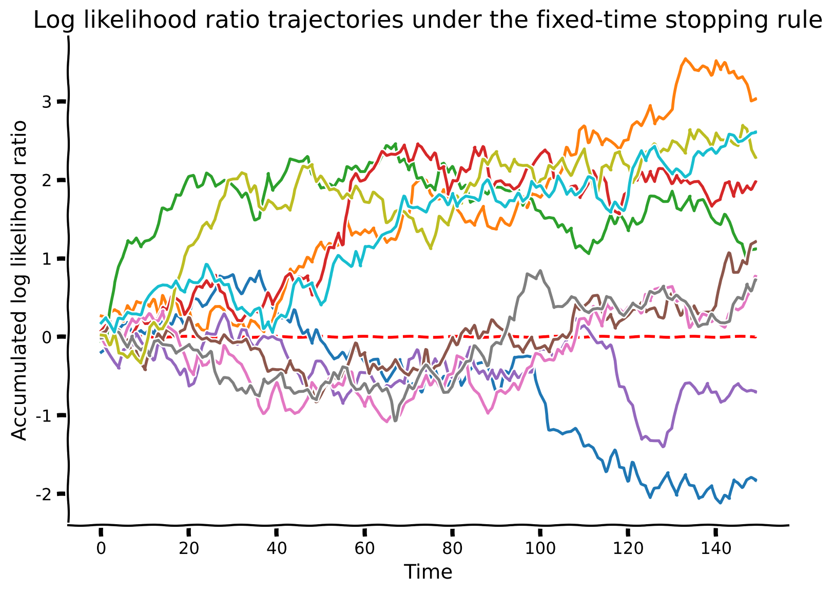
コーディング演習 1.1: SPRTモデルのシミュレーション

次に、 $s=+1$ のシミュレーションデータを生成し、SPRTが状態を正しく推定できるか試してみましょう。

simulate_SPRT_fixedtime という関数を実装します。この関数は $\mu$ , $\sigma$ , 真の状態に基づいて測定値を生成し、時間ステップごとに証拠を累積して状態の判定を出力します。判定は累積された証拠に基づいてより可能性の高い状態を選びます。次のセルで実装されている補助関数 log_likelihood_ratio を使います。これは状態が1である尤度の対数を状態が-1である尤度の対数で割ったものを計算します。

あなたのコーディングタスクは:

ステップ1: 証拠を累積する。

ステップ2: 最後の時点で判定を行う。

その後、DDMの10回のシミュレーションを可視化します。次の演習でパラメータが性能にどう影響するかを見ていきます。

# @markdown Execute this cell to enable the helper function `log_likelihood_ratio`

def log_likelihood_ratio(Mvec, p0, p1):
  """Given a sequence(vector) of observed data, calculate the log of
  likelihood ratio of p1 and p0

  Args:
    Mvec (numpy vector):           A vector of scalar measurements
    p0 (Gaussian random variable): A normal random variable with `logpdf'
                                    method
    p1 (Gaussian random variable): A normal random variable with `logpdf`
                                    method

  Returns:
    llvec: a vector of log likelihood ratios for each input data point
  """
  return p1.logpdf(Mvec) - p0.logpdf(Mvec)

def simulate_SPRT_fixedtime(mu, sigma, stop_time, true_dist = 1):
  """Simulate a Sequential Probability Ratio Test with fixed time stopping
  rule. Two observation models are 1D Gaussian distributions N(1,sigma^2) and
  N(-1,sigma^2).

  Args:
    mu (float): absolute mean value of the symmetric observation distributions
    sigma (float): Standard deviation of observation models
    stop_time (int): Number of samples to take before stopping
    true_dist (1 or -1): Which state is the true state.

  Returns:
    evidence_history (numpy vector): the history of cumulated evidence given
                                      generated data
    decision (int): 1 for s = 1, -1 for s = -1
    Mvec (numpy vector): the generated sequences of measurement data in this trial
  """

  #################################################
  ## TODO for students ##
  # Fill out function and remove
  raise NotImplementedError("Student exercise: complete simulate_SPRT_fixedtime")
  #################################################

  # Set means of observation distributions
  assert mu > 0, "Mu should be > 0"
  mu_pos = mu
  mu_neg = -mu

  # Make observation distributions
  p_pos = stats.norm(loc = mu_pos, scale = sigma)
  p_neg = stats.norm(loc = mu_neg, scale = sigma)

  # Generate a random sequence of measurements
  if true_dist == 1:
    Mvec = p_pos.rvs(size = stop_time)
  else:
    Mvec = p_neg.rvs(size = stop_time)

  # Calculate log likelihood ratio for each measurement (delta_t)
  ll_ratio_vec = log_likelihood_ratio(Mvec, p_neg, p_pos)

  # STEP 1: Calculate accumulated evidence (S) given a time series of evidence (hint: np.cumsum)
  evidence_history = ...

  # STEP 2: Make decision based on the sign of the evidence at the final time.
  decision = ...

  return evidence_history, decision, Mvec


# Set random seed
np.random.seed(100)

# Set model parameters
mu = .2
sigma = 3.5  # standard deviation for p+ and p-
num_sample = 10  # number of simulations to run
stop_time = 150 # number of steps before stopping

# Simulate and visualize
simulate_and_plot_SPRT_fixedtime(mu, sigma, stop_time, num_sample)

解答を見る$

出力例:

# @title Submit your feedback
content_review(f"{feedback_prefix}_Simulating_an_SPRT_model_Exercise")

インタラクティブデモ 1.2: 固定時間停止ルール下の軌跡

以下のデモでは、スライダーを使って観測モデルのドリフトレベル（mu）、ノイズレベル（sigma）、停止までの時間ステップ数（stop_time）を変更できます。これらのパラメータで10回のシミュレーションを観察できます。前の演習と同様に、真の状態は +1 です。

ノイズが高い場合と低い場合、誤った判定（誤った状態を選ぶ）をする可能性はどちらが高いでしょうか？
sigma が非常に小さい場合はどうなりますか？なぜでしょう？
停止までの時間ステップ数が少ない場合と多い場合、誤った判定をする可能性はどちらが高いでしょうか？

# @markdown Make sure you execute this cell to enable the widget!

def simulate_SPRT_fixedtime(mu, sigma, stop_time, true_dist=1):
  """Simulate a Sequential Probability Ratio Test with fixed time stopping
  rule. Two observation models are 1D Gaussian distributions N(1,sigma^2) and
  N(-1,sigma^2).

  Args:
    mu (float): absolute mean value of the symmetric observation distributions
    sigma (float): Standard deviation of observation models
    stop_time (int): Number of samples to take before stopping
    true_dist (1 or -1): Which state is the true state.

  Returns:
    evidence_history (numpy vector): the history of cumulated evidence given
                                      generated data
    decision (int): 1 for s = 1, -1 for s = -1
    Mvec (numpy vector): the generated sequences of measurement data in this trial
  """

  # Set means of observation distributions
  assert mu > 0, "Mu should be >0"
  mu_pos = mu
  mu_neg = -mu

  # Make observation distributions
  p_pos = stats.norm(loc = mu_pos, scale = sigma)
  p_neg = stats.norm(loc = mu_neg, scale = sigma)

  # Generate a random sequence of measurements
  if true_dist == 1:
    Mvec = p_pos.rvs(size = stop_time)
  else:
    Mvec = p_neg.rvs(size = stop_time)

  # Calculate log likelihood ratio for each measurement (delta_t)
  ll_ratio_vec = log_likelihood_ratio(Mvec, p_neg, p_pos)

  # STEP 1: Calculate accumulated evidence (S) given a time series of evidence (hint: np.cumsum)
  evidence_history = np.cumsum(ll_ratio_vec)

  # STEP 2: Make decision based on the sign of the evidence at the final time.
  decision = np.sign(evidence_history[-1])

  return evidence_history, decision, Mvec


np.random.seed(100)
num_sample = 10

@widgets.interact(mu=widgets.FloatSlider(min=0.1, max=5.0, step=0.1, value=0.5),
                  sigma=(0.05, 10.0, 0.05), stop_time=(5, 500, 1))
def plot(mu, sigma, stop_time):
  simulate_and_plot_SPRT_fixedtime(mu, sigma, stop_time,
                                   num_sample, verbose=False)

解答を見る$

# @title Submit your feedback
content_review(f"{feedback_prefix}_Trajectories_under_the_fixed_time_stopping rule_Interactive_Demo_and_Discussion")

# @title Video 3: Section 1 Exercises Discussion
from ipywidgets import widgets
from IPython.display import YouTubeVideo
from IPython.display import IFrame
from IPython.display import display


class PlayVideo(IFrame):
  def __init__(self, id, source, page=1, width=400, height=300, **kwargs):
    self.id = id
    if source == 'Bilibili':
      src = f'https://player.bilibili.com/player.html?bvid={id}&page={page}'
    elif source == 'Osf':
      src = f'https://mfr.ca-1.osf.io/render?url=https://osf.io/download/{id}/?direct%26mode=render'
    super(PlayVideo, self).__init__(src, width, height, **kwargs)


def display_videos(video_ids, W=400, H=300, fs=1):
  tab_contents = []
  for i, video_id in enumerate(video_ids):
    out = widgets.Output()
    with out:
      if video_ids[i][0] == 'Youtube':
        video = YouTubeVideo(id=video_ids[i][1], width=W,
                             height=H, fs=fs, rel=0)
        print(f'Video available at https://youtube.com/watch?v={video.id}')
      else:
        video = PlayVideo(id=video_ids[i][1], source=video_ids[i][0], width=W,
                          height=H, fs=fs, autoplay=False)
        if video_ids[i][0] == 'Bilibili':
          print(f'Video available at https://www.bilibili.com/video/{video.id}')
        elif video_ids[i][0] == 'Osf':
          print(f'Video available at https://osf.io/{video.id}')
      display(video)
    tab_contents.append(out)
  return tab_contents


video_ids = [('Youtube', 'P6xuOS5TB7Q'), ('Bilibili', 'BV1h54y1E7UC')]
tab_contents = display_videos(video_ids, W=854, H=480)
tabs = widgets.Tab()
tabs.children = tab_contents
for i in range(len(tab_contents)):
  tabs.set_title(i, video_ids[i][0])
display(tabs)

# @title Submit your feedback
content_review(f"{feedback_prefix}_Section_1_Exercises_Discussion_Video")

セクション 2: DDMの解析：正確さと停止時間の関係

チュートリアル開始からここまでの推定所要時間：28分

# @title Video 4: Speed vs Accuracy Tradeoff
from ipywidgets import widgets
from IPython.display import YouTubeVideo
from IPython.display import IFrame
from IPython.display import display


class PlayVideo(IFrame):
  def __init__(self, id, source, page=1, width=400, height=300, **kwargs):
    self.id = id
    if source == 'Bilibili':
      src = f'https://player.bilibili.com/player.html?bvid={id}&page={page}'
    elif source == 'Osf':
      src = f'https://mfr.ca-1.osf.io/render?url=https://osf.io/download/{id}/?direct%26mode=render'
    super(PlayVideo, self).__init__(src, width, height, **kwargs)


def display_videos(video_ids, W=400, H=300, fs=1):
  tab_contents = []
  for i, video_id in enumerate(video_ids):
    out = widgets.Output()
    with out:
      if video_ids[i][0] == 'Youtube':
        video = YouTubeVideo(id=video_ids[i][1], width=W,
                             height=H, fs=fs, rel=0)
        print(f'Video available at https://youtube.com/watch?v={video.id}')
      else:
        video = PlayVideo(id=video_ids[i][1], source=video_ids[i][0], width=W,
                          height=H, fs=fs, autoplay=False)
        if video_ids[i][0] == 'Bilibili':
          print(f'Video available at https://www.bilibili.com/video/{video.id}')
        elif video_ids[i][0] == 'Osf':
          print(f'Video available at https://osf.io/{video.id}')
      display(video)
    tab_contents.append(out)
  return tab_contents


video_ids = [('Youtube', 'Hc3uXQiKvZA'), ('Bilibili', 'BV1s54y1E7yT')]
tab_contents = display_videos(video_ids, W=854, H=480)
tabs = widgets.Tab()
tabs.children = tab_contents
for i in range(len(tab_contents)):
  tabs.set_title(i, video_ids[i][0])
display(tabs)

# @title Submit your feedback
content_review(f"{feedback_prefix}_Speed_vs_Accuracy_Tradeoff_Video")

もし慌てて決定を下した場合（例えば、サンプルを2つしか見ていない場合）や、観測ノイズが信号をかき消してしまった場合、累積対数尤度比が負になり、誤った決定をしてしまうことがあります。決定の正確さがサンプル数に応じてどのように変化するかをプロットしてみましょう。正確さは、繰り返しシミュレーションにおける正しい試行の割合で表されます： $\frac{\# \textrm{ 正しい決定}}{\# \textrm{ 全決定数}}$ 。

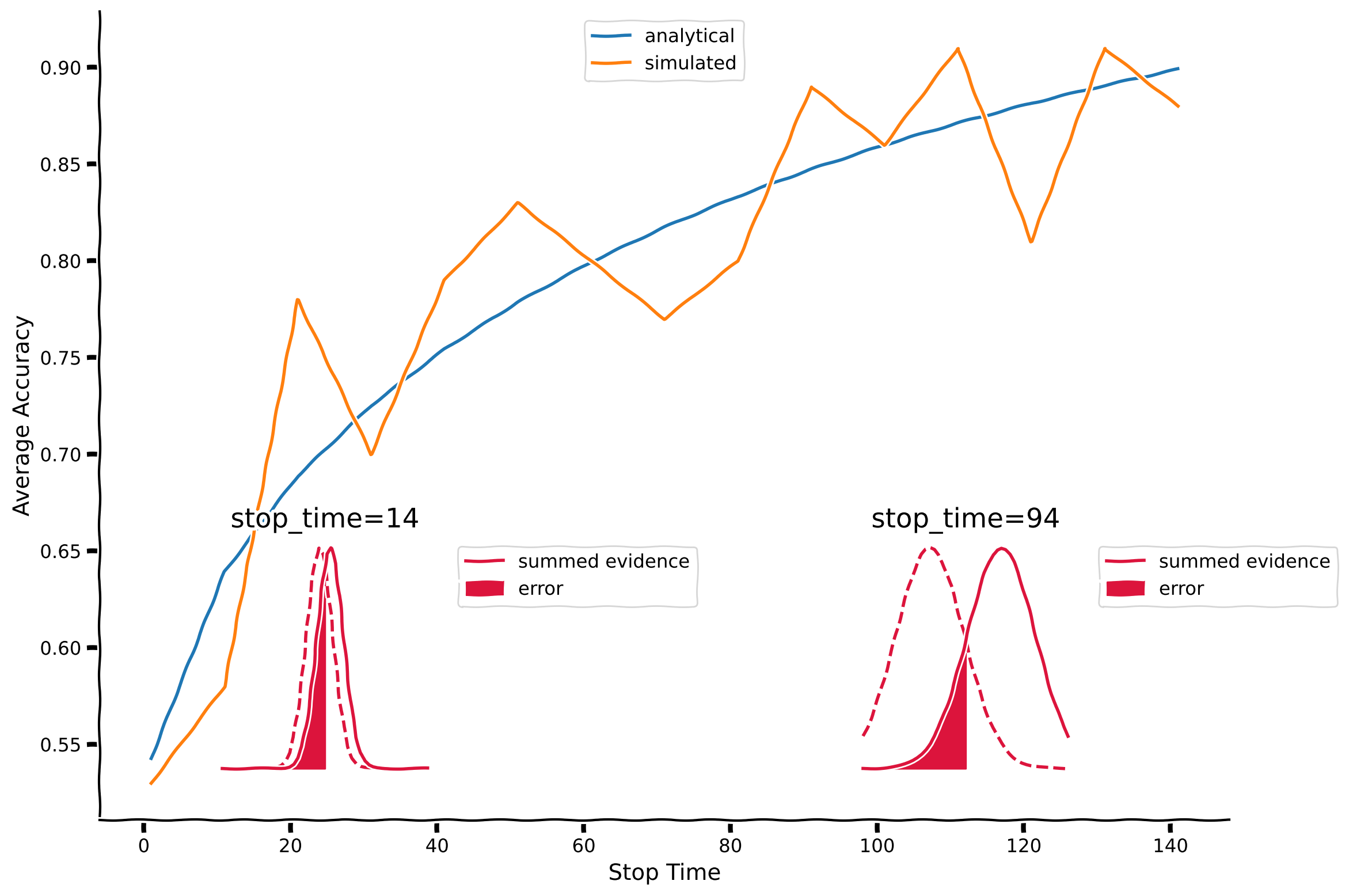
コーディング演習 2.1: 速度と正確さのトレードオフ

観測ノイズのレベルは固定します。この演習では、特定の停止時間で多数のシミュレーションを実行し、_平均決定正確さ_を計算する関数を実装します。その後、平均決定正確さと停止時間の関係を可視化します。

def simulate_accuracy_vs_stoptime(mu, sigma, stop_time_list, num_sample,
                                  no_numerical=False):
  """Calculate the average decision accuracy vs. stopping time by running
  repeated SPRT simulations for each stop time.

  Args:
      mu (float): absolute mean value of the symmetric observation distributions
      sigma (float): standard deviation for observation model
      stop_list_list (list-like object): a list of stopping times to run over
      num_sample (int): number of simulations to run per stopping time
      no_numerical (bool): flag that indicates the function to return analytical values only

  Returns:
      accuracy_list: a list of average accuracies corresponding to input
                      `stop_time_list`
      decisions_list: a list of decisions made in all trials
  """

  #################################################
  ## TODO for students##
  # Fill out function and remove
  raise NotImplementedError("Student exercise: complete simulate_accuracy_vs_stoptime")
  #################################################

  # Determine true state (1 or -1)
  true_dist = 1

  # Set up tracker of accuracy and decisions
  accuracies = np.zeros(len(stop_time_list),)
  accuracies_analytical = np.zeros(len(stop_time_list),)
  decisions_list = []

  # Loop over stop times
  for i_stop_time, stop_time in enumerate(stop_time_list):

    if not no_numerical:
      # Set up tracker of decisions for this stop time
      decisions = np.zeros((num_sample,))

      # Loop over samples
      for i in range(num_sample):

        # STEP 1: Simulate run for this stop time (hint: use output from last exercise)
        _, decision, _= ...

        # Log decision
        decisions[i] = decision

      # STEP 2: Calculate accuracy by averaging over trials
      accuracies[i_stop_time] = ...

      # Log decision
      decisions_list.append(decisions)

    # Calculate analytical accuracy
    sigma_sum_gaussian = sigma / np.sqrt(stop_time)
    accuracies_analytical[i_stop_time] = 0.5 + 0.5 * erf(mu / np.sqrt(2) / sigma_sum_gaussian)

  return accuracies, accuracies_analytical, decisions_list


# Set random seed
np.random.seed(100)

# Set parameters of model
mu = 0.5
sigma = 4.65  # standard deviation for observation noise
num_sample = 100  # number of simulations to run for each stopping time
stop_time_list = np.arange(1, 150, 10) # Array of stopping times to use


# Calculate accuracies for each stop time
accuracies, accuracies_analytical, _ = simulate_accuracy_vs_stoptime(mu, sigma, stop_time_list,
                                                   num_sample)

# Visualize
plot_accuracy_vs_stoptime(mu, sigma, stop_time_list, accuracies_analytical, accuracies)

解答を見る$

出力例:

# @title Submit your feedback
content_review(f"{feedback_prefix}_Speed_vs_Accuracy_Tradeoff_Exercise")

上図では、シミュレーションによる精度をオレンジ色でプロットしています。実は、この特定のケースにおける平均精度の解析的な方程式を求めることができ、それを青色でプロットしています。ここでは解析解の詳細には踏み込みませんが、もし多数の異なるシミュレーションを行い、同じ数のオレンジの線があったとすると、それらの平均は青い線に近いものになると想像できます。

挿入図では、ある時点における2つの状態の証拠分布を示しています。セクション1で述べたように、時刻 $T$ における状態 +1 の尤度比は次の通りです：

L_T\sim\mathcal{N}\left(2\frac{\mu^2}{\sigma^2}T,\ 4\frac{\mu^2}{\sigma^2}T\right)=\mathcal{N}(bT,c^2T)

状態が -1 の場合は平均が符号反転します。ここでは状態が -1（破線）および +1（実線）のガウス分布をプロットしています。赤色の領域は誤り率を示しており、この領域は真の状態が +1 であるにもかかわらず $L_T$ が0未満となり誤った状態を判断してしまう部分に対応します。時間が経つにつれてこれらの分布はより分離し、誤り率は低下します。

インタラクティブデモ 2.2: 精度と停止時間の関係

同じ可視化で、今度は証拠の平均 $\mu$ と標準偏差 sigma を変化させてみましょう。ノイズが低い場合と高い場合で、停止時間に対する精度のプロットはどのようになると予想しますか？

# @markdown Make sure you execute this cell to enable the widget!

def simulate_accuracy_vs_stoptime(mu, sigma, stop_time_list,
                                  num_sample, no_numerical=False):
  """Calculate the average decision accuracy vs. stopping time by running
  repeated SPRT simulations for each stop time.

  Args:
      mu (float): absolute mean value of the symmetric observation distributions
      sigma (float): standard deviation for observation model
      stop_list_list (list-like object): a list of stopping times to run over
      num_sample (int): number of simulations to run per stopping time
      no_numerical (bool): flag that indicates the function to return analytical values only

  Returns:
      accuracy_list: a list of average accuracies corresponding to input
                      `stop_time_list`
      decisions_list: a list of decisions made in all trials
  """

  # Determine true state (1 or -1)
  true_dist = 1

  # Set up tracker of accuracy and decisions
  accuracies = np.zeros(len(stop_time_list),)
  accuracies_analytical = np.zeros(len(stop_time_list),)
  decisions_list = []

  # Loop over stop times
  for i_stop_time, stop_time in enumerate(stop_time_list):

    if not no_numerical:
      # Set up tracker of decisions for this stop time
      decisions = np.zeros((num_sample,))

      # Loop over samples
      for i in range(num_sample):

        # Simulate run for this stop time (hint: last exercise)
        _, decision, _= simulate_SPRT_fixedtime(mu, sigma, stop_time, true_dist)

        # Log decision
        decisions[i] = decision

      # Calculate accuracy
      accuracies[i_stop_time] = np.sum(decisions == true_dist) / decisions.shape[0]
      # Log decisions
      decisions_list.append(decisions)

    # Calculate analytical accuracy
    sigma_sum_gaussian = sigma / np.sqrt(stop_time)
    accuracies_analytical[i_stop_time] = 0.5 + 0.5 * erf(mu / np.sqrt(2) / sigma_sum_gaussian)

  return accuracies, accuracies_analytical, decisions_list


np.random.seed(100)
num_sample = 100
stop_time_list = np.arange(1, 100, 1)

@widgets.interact
def plot(mu=widgets.FloatSlider(min=0.1, max=5.0, step=0.1, value=1.0),
         sigma=(0.05, 10.0, 0.05)):
 # Calculate accuracies for each stop time
  _, accuracies_analytical, _ = simulate_accuracy_vs_stoptime(mu, sigma,
                                                              stop_time_list,
                                                              num_sample,
                                                              no_numerical=True)
  # Visualize
  plot_accuracy_vs_stoptime(mu, sigma, stop_time_list, accuracies_analytical)

解答を見る$

# @title Submit your feedback
content_review(f"{feedback_prefix}_Speed_vs_Accuracy_Tradeoff_Interactive_Demo_and_Discussion")

# @title Video 5: Section 2 Exercises Discussion
from ipywidgets import widgets
from IPython.display import YouTubeVideo
from IPython.display import IFrame
from IPython.display import display


class PlayVideo(IFrame):
  def __init__(self, id, source, page=1, width=400, height=300, **kwargs):
    self.id = id
    if source == 'Bilibili':
      src = f'https://player.bilibili.com/player.html?bvid={id}&page={page}'
    elif source == 'Osf':
      src = f'https://mfr.ca-1.osf.io/render?url=https://osf.io/download/{id}/?direct%26mode=render'
    super(PlayVideo, self).__init__(src, width, height, **kwargs)


def display_videos(video_ids, W=400, H=300, fs=1):
  tab_contents = []
  for i, video_id in enumerate(video_ids):
    out = widgets.Output()
    with out:
      if video_ids[i][0] == 'Youtube':
        video = YouTubeVideo(id=video_ids[i][1], width=W,
                             height=H, fs=fs, rel=0)
        print(f'Video available at https://youtube.com/watch?v={video.id}')
      else:
        video = PlayVideo(id=video_ids[i][1], source=video_ids[i][0], width=W,
                          height=H, fs=fs, autoplay=False)
        if video_ids[i][0] == 'Bilibili':
          print(f'Video available at https://www.bilibili.com/video/{video.id}')
        elif video_ids[i][0] == 'Osf':
          print(f'Video available at https://osf.io/{video.id}')
      display(video)
    tab_contents.append(out)
  return tab_contents


video_ids = [('Youtube', 'OBDv6nB6a2g'), ('Bilibili', 'BV11g411M7Lm')]
tab_contents = display_videos(video_ids, W=854, H=480)
tabs = widgets.Tab()
tabs.children = tab_contents
for i in range(len(tab_contents)):
  tabs.set_title(i, video_ids[i][0])
display(tabs)

# @title Submit your feedback
content_review(f"{feedback_prefix}_Section_2_Exercises_Discussion_Video")

応用

ここまで釣り問題の文脈でドリフト拡散モデル（Drift Diffusion Model, DDM）を見てきましたが、神経科学ではこれが多くの用途で使われています。例えば、神経科学の古典的な実験課題の一つにランダムドット運動視覚課題（random dot kinematogram）があります（Newsome, Britten, Movshon 1989）。この課題では、ランダムな方向に動く多数の点のパターンが提示されますが、わずかなコヒーレンス（整合性）があり、全体として右方向または左方向への動きが優勢です。観察者はその方向を推測しなければなりません。脳内のニューロンはこの課題に関して情報を持ち、その応答は選択と相関し、ドリフト拡散モデルの予測と一致します（Huk and Shadlen 2005）。

以下は、Pamela Reinagle による、ラットがこの課題で動きの方向を推測する様子のビデオです。

# @markdown Rat performing random dot motion task
from IPython.display import YouTubeVideo
video = YouTubeVideo(id="oDxcyTn-0os", width=854, height=480, fs=1)
print("Video available at https://youtu.be/" + video.id)
video

他のチュートリアルを終えたら、ボーナス教材に戻って、DDMの別の停止ルールである「確信度に基づく固定閾値」について学びましょう。

まとめ

チュートリアルの推定所要時間：45分

よくできました！ドリフト拡散モデルをシミュレーションすることで、以下のことを学びました：

2つの候補モデルの対数尤度比として個々のサンプル証拠を計算する方法
新しいデータ点から証拠を蓄積し、再帰的な公式を用いて事後確率を計算する方法
繰り返しシミュレーションを行い、意思決定の精度を推定する方法
速度と精度のトレードオフを測定する方法

ボーナス

ボーナスセクション 1: 信頼度の固定閾値を用いたDDM

# @title Video 6: Fixed threshold on confidence
from ipywidgets import widgets
from IPython.display import YouTubeVideo
from IPython.display import IFrame
from IPython.display import display


class PlayVideo(IFrame):
  def __init__(self, id, source, page=1, width=400, height=300, **kwargs):
    self.id = id
    if source == 'Bilibili':
      src = f'https://player.bilibili.com/player.html?bvid={id}&page={page}'
    elif source == 'Osf':
      src = f'https://mfr.ca-1.osf.io/render?url=https://osf.io/download/{id}/?direct%26mode=render'
    super(PlayVideo, self).__init__(src, width, height, **kwargs)


def display_videos(video_ids, W=400, H=300, fs=1):
  tab_contents = []
  for i, video_id in enumerate(video_ids):
    out = widgets.Output()
    with out:
      if video_ids[i][0] == 'Youtube':
        video = YouTubeVideo(id=video_ids[i][1], width=W,
                             height=H, fs=fs, rel=0)
        print(f'Video available at https://youtube.com/watch?v={video.id}')
      else:
        video = PlayVideo(id=video_ids[i][1], source=video_ids[i][0], width=W,
                          height=H, fs=fs, autoplay=False)
        if video_ids[i][0] == 'Bilibili':
          print(f'Video available at https://www.bilibili.com/video/{video.id}')
        elif video_ids[i][0] == 'Osf':
          print(f'Video available at https://osf.io/{video.id}')
      display(video)
    tab_contents.append(out)
  return tab_contents


video_ids = [('Youtube', 'E8lvgFeIGQM'), ('Bilibili', 'BV1Ya4y1a7c1')]
tab_contents = display_videos(video_ids, W=854, H=480)
tabs = widgets.Tab()
tabs.children = tab_contents
for i in range(len(tab_contents)):
  tabs.set_title(i, video_ids[i][0])
display(tabs)

# @title Submit your feedback
content_review(f"{feedback_prefix}_Fixed_threshold_on_confidence_Bonus_Video")

次の演習では、固定された意思決定時間の代わりに固定された信頼度閾値を用いるDDMの変種を考えます。これは神経統合のより良い記述となるかもしれません。このトピックに関して追加情報が欲しい場合は、すべてのチュートリアルのメインコンテンツを終えた後にこの資料を完成させてください。

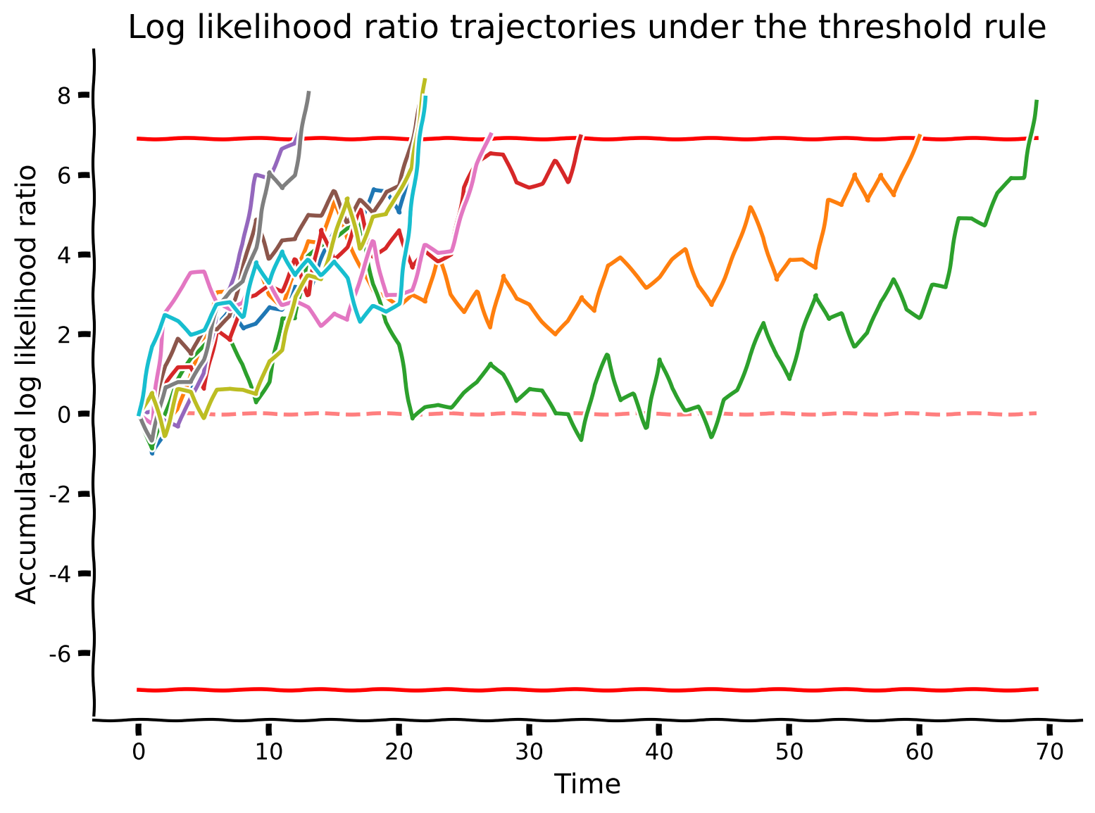
ボーナスコーディング演習 1.1: 固定信頼度閾値を用いたDDMのシミュレーション

ビデオ中の演習3として言及されています

この演習では、停止ルールとして閾値判定を用い、DDMの挙動を観察します。

閾値判定停止ルールでは、望ましい誤差率を定義し、その誤差率に達するまで測定を続けます。実験的証拠は、証拠の蓄積と閾値判定停止戦略が神経レベルで起こっていることを示唆しています（詳細はこちらの記事を参照）。

関数 threshold_from_errorrate を完成させ、望ましい誤差率 $\alpha$ から証拠の閾値を以下の式に従って計算してください。証拠の閾値 $th_1$ と $th_0$ は $p_+$ と $p_-$ に対して互いに逆符号であるため、絶対値を返せば十分です。

\begin{align}
$th_{L}$ &= $\log \frac{\alpha}{1-\alpha} = -th_{R}$ \
$th_{R}$ &= $\log \frac{1-\alpha}{\alpha} = -th_{1}
\end{align}

*$ 関数 simulate_SPRT_threshold を完成させ、ノイズレベルと望ましい閾値を与えて閾値判定停止ルールを用いたSPRTをシミュレートしてください。

指定されたノイズレベルと望ましい誤差率に対して繰り返しシミュレーションを実行し、提供されたコードを用いてDDMのトレースを可視化してください。

def simulate_SPRT_threshold(mu, sigma, threshold , true_dist=1):
  """Simulate a Sequential Probability Ratio Test with thresholding stopping
  rule. Two observation models are 1D Gaussian distributions N(1,sigma^2) and
  N(-1,sigma^2).

  Args:
    mu (float): absolute mean value of the symmetric observation distributions
    sigma (float): Standard deviation
    threshold (float): Desired log likelihood ratio threshold to achieve
                        before making decision

  Returns:
    evidence_history (numpy vector): the history of cumulated evidence given
                                      generated data
    decision (int): 1 for pR, 0 for pL
    data (numpy vector): the generated sequences of data in this trial
  """
  assert mu > 0, "Mu should be > 0"
  muL = -mu
  muR = mu

  pL = stats.norm(muL, sigma)
  pR = stats.norm(muR, sigma)

  has_enough_data = False

  data_history = []
  evidence_history = []
  current_evidence = 0.0

  # Keep sampling data until threshold is crossed
  while not has_enough_data:
    if true_dist == 1:
      Mvec = pR.rvs()
    else:
      Mvec = pL.rvs()

    ########################################################################
    # Insert your code here to:
    #      * Calculate the log-likelihood ratio for the new sample
    #      * Update the accumulated evidence
    raise NotImplementedError("`simulate_SPRT_threshold` is incomplete")
    ########################################################################

    # STEP 1: individual log likelihood ratios
    ll_ratio = log_likelihood_ratio(...)

    # STEP 2: accumulated evidence for this chunk
    evidence_history.append(...)

    # update the collection of all data
    data_history.append(Mvec)
    current_evidence = evidence_history[-1]

    # check if we've got enough data
    if abs(current_evidence) > threshold:
      has_enough_data = True

  data_history = np.array(data_history)
  evidence_history = np.array(evidence_history)

  # Make decision
  if evidence_history[-1] >= 0:
    decision = 1
  elif evidence_history[-1] < 0:
    decision = 0

  return evidence_history, decision, data_history


# Set parameters
np.random.seed(100)
mu = 1.0
sigma = 2.8
num_sample = 10
log10_alpha = -3 # log10(alpha)
alpha = np.power(10.0, log10_alpha)

# Simulate and visualize
simulate_and_plot_SPRT_fixedthreshold(mu, sigma, num_sample, alpha)

解答を見る$

出力例:

# @title Submit your feedback
content_review(f"{feedback_prefix}_Simulating_the_DDM_with_fixed_confidence_thresholds_Bonus_Exercise")

ボーナスインタラクティブデモ 1.2: 固定信頼度閾値を用いたDDM

alpha と sigma の異なる値を操作し、ドリフト拡散モデルのダイナミクスにどのような影響があるか観察してください。

# @markdown Make sure you execute this cell to enable the widget!
def simulate_SPRT_threshold(mu, sigma, threshold , true_dist=1):
  """Simulate a Sequential Probability Ratio Test with thresholding stopping
  rule. Two observation models are 1D Gaussian distributions N(1,sigma^2) and
  N(-1,sigma^2).

  Args:
    mu (float): absolute mean value of the symmetric observation distributions
    sigma (float): Standard deviation
    threshold (float): Desired log likelihood ratio threshold to achieve
                        before making decision

  Returns:
    evidence_history (numpy vector): the history of cumulated evidence given
                                      generated data
    decision (int): 1 for pR, 0 for pL
    data (numpy vector): the generated sequences of data in this trial
  """
  assert mu > 0, "Mu should be > 0"
  muL = -mu
  muR = mu

  pL = stats.norm(muL, sigma)
  pR = stats.norm(muR, sigma)

  has_enough_data = False

  data_history = []
  evidence_history = []
  current_evidence = 0.0

  # Keep sampling data until threshold is crossed
  while not has_enough_data:
    if true_dist == 1:
      Mvec = pR.rvs()
    else:
      Mvec = pL.rvs()

    # STEP 1: individual log likelihood ratios
    ll_ratio = log_likelihood_ratio(Mvec, pL, pR)

    # STEP 2: accumulated evidence for this chunk
    evidence_history.append(ll_ratio + current_evidence)

    # update the collection of all data
    data_history.append(Mvec)
    current_evidence = evidence_history[-1]

    # check if we've got enough data
    if abs(current_evidence) > threshold:
      has_enough_data = True

  data_history = np.array(data_history)
  evidence_history = np.array(evidence_history)

  # Make decision
  if evidence_history[-1] >= 0:
    decision = 1
  elif evidence_history[-1] < 0:
    decision = 0

  return evidence_history, decision, data_history

np.random.seed(100)
num_sample = 10

@widgets.interact
def plot(mu=(0.1,5.0,0.1), sigma=(0.05, 10.0, 0.05), log10_alpha=(-8, -1, .1)):
  alpha = np.power(10.0, log10_alpha)
  simulate_and_plot_SPRT_fixedthreshold(mu, sigma, num_sample, alpha, verbose=False)

# @title Submit your feedback
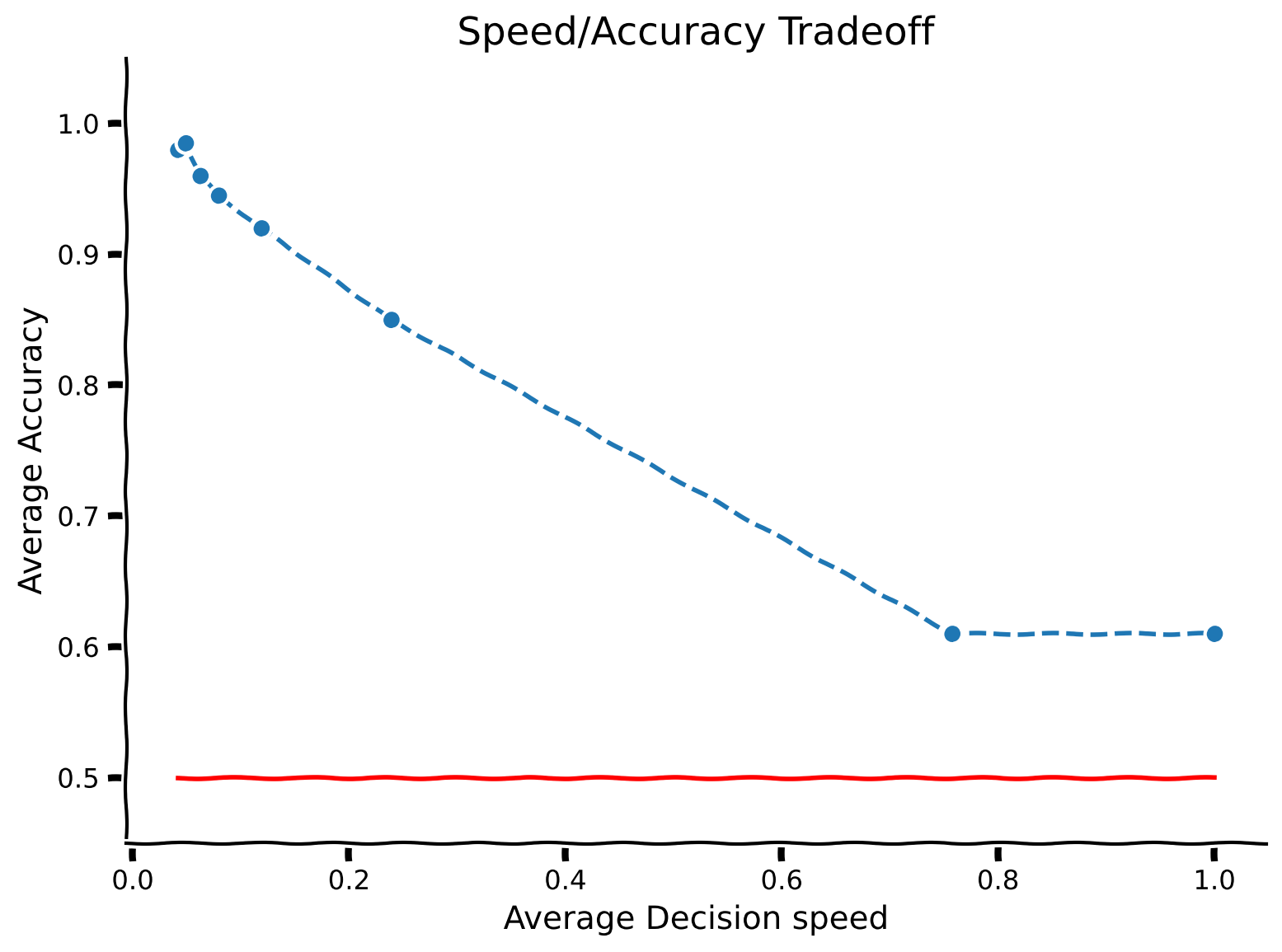
content_review(f"{feedback_prefix}_DDM_with_fixed_confidence_threshold_Bonus_Interactive_Demo")

ボーナスコーディング演習 1.3: 速度/精度トレードオフの再考

意思決定を速く行うほど、精度は低くなることが多いです。この現象は速度/精度トレードオフとして知られています。人間は幅広い状況でこのトレードオフを行い、アリ、ミツバチ、齧歯類、サルなど多くの動物種も同様の効果を示します。

閾値判定停止ルールの下で速度/精度トレードオフを示すために、異なる閾値でシミュレーションを行い、平均意思決定「速度」（1/長さ）が平均意思決定精度とどのように変化するかを見てみましょう。実験では、被験者は速くまたは遅く反応するよう動機付けられることがあり、意思決定時間や誤差閾値を正確に制御することは非常に難しいため、速度を用います。

関数 simulate_accuracy_vs_threshold を完成させ、誤差閾値のリストに対して平均精度と平均意思決定長さをシミュレートして計算してください。試行の長さから平均意思決定『速度』を計算するコードを追加する必要があります。また、これらの試行全体の精度も計算してください。
誤差閾値のリストを設定しています。繰り返しシミュレーションを実行し、各誤差率に対して平均精度と平均長さを収集し、提供されたコードを用いて速度/精度トレードオフを可視化してください。長さと精度の間に正の相関が見られるはずです。

def simulate_accuracy_vs_threshold(mu, sigma, threshold_list, num_sample):
  """Calculate the average decision accuracy vs. average decision length by
  running repeated SPRT simulations with thresholding stopping rule for each
  threshold.

  Args:
      mu (float): absolute mean value of the symmetric observation distributions
      sigma (float): standard deviation for observation model
      threshold_list (list-like object): a list of evidence thresholds to run
                                          over
      num_sample (int): number of simulations to run per stopping time

  Returns:
      accuracy_list: a list of average accuracies corresponding to input
                      `threshold_list`
      decision_speed_list: a list of average decision speeds
  """
  decision_speed_list = []
  accuracy_list = []
  for threshold in threshold_list:
    decision_time_list = []
    decision_list = []
    for i in range(num_sample):
      # run simulation and get decision of current simulation
      _, decision, Mvec = simulate_SPRT_threshold(mu, sigma, threshold)
      decision_time = len(Mvec)
      decision_list.append(decision)
      decision_time_list.append(decision_time)

    ########################################################################
    # Insert your code here to:
    #      * Calculate mean decision speed given a list of decision times
    #      * Hint: Think about speed as being inversely proportional
    #        to decision_length. If it takes 10 seconds to make one decision,
    #        our "decision speed" is 0.1 decisions per second.
    #      * Calculate the decision accuracy
    raise NotImplementedError("`simulate_accuracy_vs_threshold` is incomplete")
    ########################################################################
    # Calculate and store average decision speed and accuracy
    decision_speed = ...
    decision_accuracy = ...
    decision_speed_list.append(decision_speed)
    accuracy_list.append(decision_accuracy)

  return accuracy_list, decision_speed_list


# Set parameters
np.random.seed(100)
mu = 1.0
sigma = 3.75
num_sample = 200
alpha_list = np.logspace(-2, -0.1, 8)
threshold_list = threshold_from_errorrate(alpha_list)

# Simulate and visualize
simulate_and_plot_accuracy_vs_threshold(mu, sigma, threshold_list, num_sample)

解答を見る$

出力例:

# @title Submit your feedback
content_review(f"{feedback_prefix}_Speed_vs_Accuracy_Tradeoff_Revisited_Bonus_Exercise")

ボーナスインタラクティブデモ 1.4: 閾値ルールによる速度/精度トレードオフ

ノイズレベル sigma を操作し、それが速度/精度トレードオフにどのような影響を与えるか観察してください。

# @markdown Make sure you execute this cell to enable the widget!
def simulate_accuracy_vs_threshold(mu, sigma, threshold_list, num_sample):
  """Calculate the average decision accuracy vs. average decision speed by
  running repeated SPRT simulations with thresholding stopping rule for each
  threshold.

  Args:
      mu (float): absolute mean value of the symmetric observation distributions
      sigma (float): standard deviation for observation model
      threshold_list (list-like object): a list of evidence thresholds to run
                                          over
      num_sample (int): number of simulations to run per stopping time

  Returns:
      accuracy_list: a list of average accuracies corresponding to input
                      `threshold_list`
      decision_speed_list: a list of average decision speeds
  """
  decision_speed_list = []
  accuracy_list = []
  for threshold in threshold_list:
    decision_time_list = []
    decision_list = []
    for i in range(num_sample):
      # run simulation and get decision of current simulation
      _, decision, Mvec = simulate_SPRT_threshold(mu, sigma, threshold)
      decision_time = len(Mvec)
      decision_list.append(decision)
      decision_time_list.append(decision_time)

    # Calculate and store average decision speed and accuracy
    decision_speed = np.mean(1. / np.array(decision_time_list))
    decision_accuracy = sum(decision_list) / len(decision_list)
    decision_speed_list.append(decision_speed)
    accuracy_list.append(decision_accuracy)

  return accuracy_list, decision_speed_list


np.random.seed(100)
num_sample = 100
alpha_list = np.logspace(-2, -0.1, 8)
threshold_list = threshold_from_errorrate(alpha_list)

@widgets.interact
def plot(mu=(0.1, 5.0, 0.1), sigma=(0.05, 10.0, 0.05)):
  alpha = np.power(10.0, log10_alpha)
  simulate_and_plot_accuracy_vs_threshold(mu, sigma, threshold_list, num_sample)

# @title Submit your feedback
content_review(f"{feedback_prefix}_Speed_vs_Accuracy_with_a_threshold_rule_Bonus_Interactive_Demo")