ボーナスチュートリアル: データへのフィッティング

第3週、第2日目: ベイズ的意思決定

Neuromatch Academyによる

コンテンツ作成者: Vincent Valton, Konrad Kording

コンテンツレビュアー: Matt Krause, Jesse Livezey, Karolina Stosio, Saeed Salehi, Michael Waskom

制作編集: Gagana B, Spiros Chavlis

注意: これはNMA 2020からのボーナスマテリアルであり、大幅な改訂はされていません。したがって、表記や基準がやや異なり、NMAの他の日の参照が古くなっている部分があります。ここに含めているのは、ベイズモデルをデータにフィットさせる方法を扱っており、多くの学生にとって興味深い内容だからです。

チュートリアルの目的

最初の2つのチュートリアルでは、デモを使ってベイズモデルと意思決定をより直感的に学びました。このノートブックでは、数学とコードを使ってベイズモデルをデータにフィットさせる方法に踏み込みます。

モデルの逆問題（参加者のデータに似たデータを生成したモデルパラメータ、例えば $p_{common}$ を推定する）を実行するために必要なすべてのステップを計算していきます。まず生成モデルのすべてのステップを説明し、最後の演習でこれらのステップを使ってシミュレートされたデータから単一参加者のパラメータ $p_{common}$ を推定します。

生成モデルはチュートリアル2で見たベイズモデルで、ガウス混合事前分布とガウス尤度の組み合わせです。

ステップ:

まず、生成モデルの各ステップで計算・推定されるものを視覚化しやすくするために、事前分布、尤度、事後分布などを作成します:
1. 複数の可能な刺激入力に対するガウス混合事前分布の作成
2. 複数の可能な刺激入力に対する尤度の生成
3. 刺激入力の関数として事後分布の推定
4. 事後分布に基づく参加者の応答の推定
次に、モデルの逆問題／フィッティングを行います:
5. 可能な入力の関数として入力の分布を作成
6. 周辺化
7. 提供された生成モデルを使ってデータを生成
8. 生成データを用いてモデルの逆問題（フィッティング）を実行し、元のパラメータを回復できるか確認

# @title Tutorial slides
# @markdown These are the slides for the videos in this tutorial
from IPython.display import IFrame
link_id = "sqnd5"
print(f"If you want to download the slides: https://osf.io/download/{link_id}/")
IFrame(src=f"https://mfr.ca-1.osf.io/render?url=https://osf.io/{link_id}/?direct%26mode=render%26action=download%26mode=render", width=854, height=480)

セットアップ

# @title Install and import feedback gadget


from vibecheck import DatatopsContentReviewContainer
def content_review(notebook_section: str):
    return DatatopsContentReviewContainer(
        "",  # No text prompt
        notebook_section,
        {
            "url": "https://pmyvdlilci.execute-api.us-east-1.amazonaws.com/klab",
            "name": "neuromatch_cn",
            "user_key": "y1x3mpx5",
        },
    ).render()


feedback_prefix = "W3D1_T3_Bonus"

# Imports
import numpy as np
import matplotlib.pyplot as plt
import matplotlib as mpl
from scipy.optimize import minimize

# @title Figure Settings
import logging
logging.getLogger('matplotlib.font_manager').disabled = True

import ipywidgets as widgets
%matplotlib inline
%config InlineBackend.figure_format = 'retina'
plt.style.use("https://raw.githubusercontent.com/NeuromatchAcademy/course-content/NMA2020/nma.mplstyle")

# @title Plotting functions

def plot_myarray(array, xlabel, ylabel, title):
  """ Plot an array with labels.

  Args :
    array (numpy array of floats)
    xlabel (string) - label of x-axis
    ylabel (string) - label of y-axis
    title  (string) - title of plot

  Returns:
    None
  """
  fig = plt.figure()
  ax = fig.add_subplot(111)
  colormap = ax.imshow(array, extent=[-10, 10, 8, -8])
  cbar = plt.colorbar(colormap, ax=ax)
  cbar.set_label('probability')
  ax.invert_yaxis()
  ax.set_xlabel(xlabel)
  ax.set_title(title)
  ax.set_ylabel(ylabel)
  ax.set_aspect('auto')
  return None


def plot_my_bayes_model(model) -> None:
  """Pretty-print a simple Bayes Model (ex 7), defined as a function:

  Args:
    - model: function that takes a single parameter value and returns
             the negative log-likelihood of the model, given that parameter
  Returns:
    None, draws plot
    """
  x = np.arange(-10,10,0.07)

  # Plot neg-LogLikelihood for different values of alpha
  alpha_tries = np.arange(0.01, 0.3, 0.01)
  nll = np.zeros_like(alpha_tries)
  for i_try in np.arange(alpha_tries.shape[0]):
    nll[i_try] = model(np.array([alpha_tries[i_try]]))

  plt.figure()
  plt.plot(alpha_tries, nll)
  plt.xlabel('p_independent value')
  plt.ylabel('negative log-likelihood')

  # Mark minima
  ix = np.argmin(nll)
  plt.scatter(alpha_tries[ix], nll[ix], c='r', s=144)

  #plt.axvline(alpha_tries[np.argmin(nll)])
  plt.title('Sample Output')
  plt.show()

  return None


def plot_simulated_behavior(true_stim, behaviour):
  fig = plt.figure(figsize=(7, 7))
  ax = fig.add_subplot(1,1,1)
  ax.set_facecolor('xkcd:light grey')
  plt.plot(true_stim, true_stim - behaviour, '-k', linewidth=2, label='data')
  plt.axvline(0, ls='dashed', color='grey')
  plt.axhline(0, ls='dashed', color='grey')
  plt.legend()
  plt.xlabel('Position of true visual stimulus (cm)')
  plt.ylabel('Participant deviation from true stimulus (cm)')
  plt.title('Participant behavior')
  plt.show()

  return None

# @title Helper Functions

def my_gaussian(x_points, mu, sigma):
    """
    Returns a Gaussian estimated at points `x_points`, with parameters: `mu` and `sigma`

    Args :
      x_points (numpy arrays of floats)- points at which the gaussian is evaluated
      mu (scalar) - mean of the Gaussian
      sigma (scalar) - std of the gaussian

    Returns:
      Gaussian evaluated at `x`
    """
    p = np.exp(-(x_points-mu)**2/(2*sigma**2))
    return p / sum(p)


def moments_myfunc(x_points, function):
  """
  DO NOT EDIT THIS FUNCTION !!!

  Returns the mean, median and mode of an arbitrary function

  Args :
    x_points (numpy array of floats) - x-axis values
    function (numpy array of floats) - y-axis values of the function evaluated at `x_points`

  Returns:
    (tuple of 3 scalars): mean, median, mode
  """

  # Calc mode of arbitrary function
  mode = x_points[np.argmax(function)]

  # Calc mean of arbitrary function
  mean = np.sum(x_points * function)

  # Calc median of arbitrary function
  cdf_function = np.zeros_like(x_points)
  accumulator = 0
  for i in np.arange(x_points.shape[0]):
    accumulator = accumulator + function[i]
    cdf_function[i] = accumulator
  idx = np.argmin(np.abs(cdf_function - 0.5))
  median = x_points[idx]

  return mean, median, mode

はじめに

# @title Video 1: Intro
from ipywidgets import widgets
from IPython.display import YouTubeVideo
from IPython.display import IFrame
from IPython.display import display


class PlayVideo(IFrame):
  def __init__(self, id, source, page=1, width=400, height=300, **kwargs):
    self.id = id
    if source == 'Bilibili':
      src = f'https://player.bilibili.com/player.html?bvid={id}&page={page}'
    elif source == 'Osf':
      src = f'https://mfr.ca-1.osf.io/render?url=https://osf.io/download/{id}/?direct%26mode=render'
    super(PlayVideo, self).__init__(src, width, height, **kwargs)


def display_videos(video_ids, W=400, H=300, fs=1):
  tab_contents = []
  for i, video_id in enumerate(video_ids):
    out = widgets.Output()
    with out:
      if video_ids[i][0] == 'Youtube':
        video = YouTubeVideo(id=video_ids[i][1], width=W,
                             height=H, fs=fs, rel=0)
        print(f'Video available at https://youtube.com/watch?v={video.id}')
      else:
        video = PlayVideo(id=video_ids[i][1], source=video_ids[i][0], width=W,
                          height=H, fs=fs, autoplay=False)
        if video_ids[i][0] == 'Bilibili':
          print(f'Video available at https://www.bilibili.com/video/{video.id}')
        elif video_ids[i][0] == 'Osf':
          print(f'Video available at https://osf.io/{video.id}')
      display(video)
    tab_contents.append(out)
  return tab_contents


video_ids = [('Youtube', 'YSKDhnbjKmA'), ('Bilibili', 'BV13g4y1i7je')]
tab_contents = display_videos(video_ids, W=854, H=480)
tabs = widgets.Tab()
tabs.children = tab_contents
for i in range(len(tab_contents)):
  tabs.set_title(i, video_ids[i][0])
display(tabs)

# @title Submit your feedback
content_review(f"{feedback_prefix}_Intro_Video")

生成モデルのグラフィカルな表現は以下の通りです:

刺激 $x$ を参加者に提示します。
脳はこの真の刺激 $x$ をノイズを伴って符号化します（これが脳による真の視覚刺激の表現です: $p(\tilde x|x)$ ）。
脳はこの脳で符号化された刺激（尤度: $p(\tilde x|x)$ ）と事前情報（事前分布: $p(x)$ ）を組み合わせて、真の視覚刺激の脳による推定位置、すなわち事後分布: $p(x|\tilde x)$ を作り出します。
この脳による推定刺激位置: $p(x|\tilde x)$ を用いて応答 $\hat x$ を生成します。これは参加者の刺激位置に対するノイズを含む推定（参加者の知覚）です。

通常、応答 $\hat x$ には運動ノイズ（手や腕の動きが100%正確でないことによるノイズ）も含まれますが、本チュートリアルではこれを無視し、運動ノイズがないと仮定します。

チュートリアル2$ と同じ実験設定を使いますが、確率が少し異なります。今回は、参加者はカーテンの後ろに隠れたパペットの音の位置を推定するよう指示されます。参加者は聴覚情報を使うように言われ、音は2つの原因から来る可能性があると知らされます：共通原因（95%の確率でカーテンの後ろ、位置0に隠れたパペットからの音）か独立原因（5%の確率でより遠い場所にあるスピーカーからの音）。

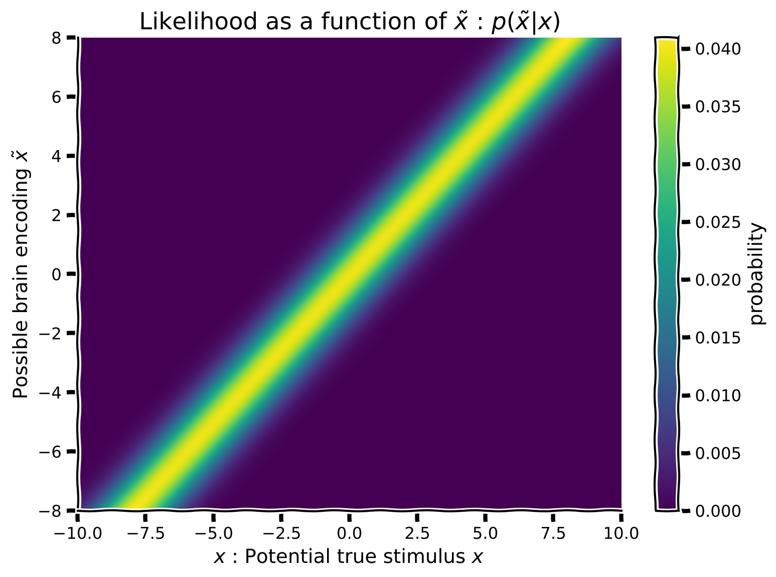
セクション1: 尤度配列

まず、尤度を作成しますが、可視化のため（およびすべての可能な脳の符号化を考慮するため）複数の尤度 $f(x)=p(\tilde x|x)$ を作成します（各潜在的符号化刺激 $\tilde x$ ごとに1つ）。これにより、仮定される真の刺激位置 $x$ をx軸に、符号化位置 $\tilde x$ をy軸にした尤度の関数を可視化できます。

my_gaussian の式と hypothetical_stim の値を使って:

平均を hypothetical_stim で変化させ、 $\sigma_{likelihood}$ は1に固定したガウス尤度を作成してください。
各尤度は異なる平均を持つため、2D配列の各行が異なる平均のガウス分布となり、合計で1,000行の異なる平均を持つ尤度配列ができます。（ヒント：np.tile はここでは使えません。forループが必要かもしれません）
すでにスクリプト内にコメントアウトされている $plot_myarray()$ 関数を使って配列をプロットしてください。

コーディング演習1: 真の刺激位置の関数として聴覚尤度を実装する

x = np.arange(-10, 10, 0.1)
hypothetical_stim = np.linspace(-8, 8, 1000)

def compute_likelihood_array(x_points, stim_array, sigma=1.):

  # initializing likelihood_array
  likelihood_array = np.zeros((len(stim_array), len(x_points)))
  # looping over stimulus array
  for i in range(len(stim_array)):
    ########################################################################
    ## Insert your code here to:
    ##      - Generate a likelihood array using `my_gaussian` function,
    ##        with std=1, and varying the mean using `stim_array` values.
    ## remove the raise below to test your function
    raise NotImplementedError("You need to complete the function!")
    ########################################################################
    likelihood_array[i, :] = ...

  return likelihood_array



likelihood_array = compute_likelihood_array(x, hypothetical_stim)
plot_myarray(likelihood_array,
             '$x$ : Potential true stimulus $x$',
             'Possible brain encoding $\~x$',
             'Likelihood as a function of $\~x$ : $p(\~x | x)$')

解答を見る$

出力例:

# @title Submit your feedback
content_review(f"{feedback_prefix}_Auditory_likelihood_Exercise")

セクション 2: ガウス事前分布の因果混合

# @title Video 2: Prior array
from ipywidgets import widgets
from IPython.display import YouTubeVideo
from IPython.display import IFrame
from IPython.display import display


class PlayVideo(IFrame):
  def __init__(self, id, source, page=1, width=400, height=300, **kwargs):
    self.id = id
    if source == 'Bilibili':
      src = f'https://player.bilibili.com/player.html?bvid={id}&page={page}'
    elif source == 'Osf':
      src = f'https://mfr.ca-1.osf.io/render?url=https://osf.io/download/{id}/?direct%26mode=render'
    super(PlayVideo, self).__init__(src, width, height, **kwargs)


def display_videos(video_ids, W=400, H=300, fs=1):
  tab_contents = []
  for i, video_id in enumerate(video_ids):
    out = widgets.Output()
    with out:
      if video_ids[i][0] == 'Youtube':
        video = YouTubeVideo(id=video_ids[i][1], width=W,
                             height=H, fs=fs, rel=0)
        print(f'Video available at https://youtube.com/watch?v={video.id}')
      else:
        video = PlayVideo(id=video_ids[i][1], source=video_ids[i][0], width=W,
                          height=H, fs=fs, autoplay=False)
        if video_ids[i][0] == 'Bilibili':
          print(f'Video available at https://www.bilibili.com/video/{video.id}')
        elif video_ids[i][0] == 'Osf':
          print(f'Video available at https://osf.io/{video.id}')
      display(video)
    tab_contents.append(out)
  return tab_contents


video_ids = [('Youtube', 'F0IYpUicXu4'), ('Bilibili', 'BV1WA411e7gM')]
tab_contents = display_videos(video_ids, W=854, H=480)
tabs = widgets.Tab()
tabs.children = tab_contents
for i in range(len(tab_contents)):
  tabs.set_title(i, video_ids[i][0])
display(tabs)

# @title Submit your feedback
content_review(f"{feedback_prefix}_Prior_array_Video")

チュートリアル2と同様に、参加者の事前知識を表す事前分布を作成したいと思います。つまり、95%の確率で音はパペットの周りの共通の位置から発生し、残りの5%の確率で別の独立した位置から発生するという情報です。この情報をガウス混合分布を用いた事前分布に組み込みます。可視化のために、前の演習で作成した尤度配列と同じ形状（フォルム）を持つ事前分布を作成します。つまり、脳が符号化した刺激 $\tilde x$ の関数としてガウス混合事前分布を作成したいのです。事前分布は $\tilde x$ に依存しないため、事前分布の2次元配列の各行は同一になります。

ガウス関数 my_gaussian の式を使って：

平均0、標準偏差0.5のガウス分布 $Common$ を生成する
平均0、標準偏差10の別のガウス分布 $Independent$ を生成する
これら2つのガウス分布（Common + Independent）を混合パラメータ $p_{independent} = 0.05$ で混合して新しい事前分布を作成する。ピーキーなガウス分布が95%の重みを持つようにし（後で正規化することを忘れずに）
これが事前分布2次元配列の最初の行になる
次に、脳符号化 $\tilde x$ を変化させてこれを繰り返す。事前分布は $\tilde x$ に依存しないので、その行の事前分布を $\tilde x$ の数（ヒント：np.tileを使う）だけ繰り返して、1,000行（つまり hypothetical_stim.shape[0]）の行事前分布配列を作成する
既にスクリプト内にコメントアウトされている関数 $plot_myarray()$ を使って行列をプロットする

コーディング演習 2: 事前配列の実装

def calculate_prior_array(x_points, stim_array, p_indep,
                          prior_mean_common=.0, prior_sigma_common=.5,
                          prior_mean_indep=.0, prior_sigma_indep=10):
  """
      'common' stands for common
      'indep' stands for independent
  """

  prior_common = my_gaussian(x_points, prior_mean_common, prior_sigma_common)
  prior_indep = my_gaussian(x_points, prior_mean_indep, prior_sigma_indep)
  ############################################################################
  ## Insert your code here to:
  ##      - Create a mixture of gaussian priors from 'prior_common'
  ##        and 'prior_indep' with mixing parameter 'p_indep'
  ##      - normalize
  ##      - repeat the prior array and reshape it to make a 2D array
  ##        of 1000 rows of priors (Hint: use np.tile() and np.reshape())
  ## remove the raise below to test your function
  raise NotImplementedError("You need to complete the function!")
  ############################################################################
  prior_mixed = ...
  prior_mixed /= ...  # normalize

  prior_array = np.tile(...).reshape(...)
  return prior_array


x = np.arange(-10, 10, 0.1)
p_independent = .05
prior_array = calculate_prior_array(x, hypothetical_stim, p_independent)
plot_myarray(prior_array,
             'Hypothesized position $x$', 'Brain encoded position $\~x$',
             'Prior as a fcn of $\~x$ : $p(x|\~x)$')

解答を見る$

出力例:

# @title Submit your feedback
content_review(f"{feedback_prefix}_Implement_Prior_array_Exercise")

セクション3: ベイズの定理と事後分布配列

# @title Video 3: Posterior array
from ipywidgets import widgets
from IPython.display import YouTubeVideo
from IPython.display import IFrame
from IPython.display import display


class PlayVideo(IFrame):
  def __init__(self, id, source, page=1, width=400, height=300, **kwargs):
    self.id = id
    if source == 'Bilibili':
      src = f'https://player.bilibili.com/player.html?bvid={id}&page={page}'
    elif source == 'Osf':
      src = f'https://mfr.ca-1.osf.io/render?url=https://osf.io/download/{id}/?direct%26mode=render'
    super(PlayVideo, self).__init__(src, width, height, **kwargs)


def display_videos(video_ids, W=400, H=300, fs=1):
  tab_contents = []
  for i, video_id in enumerate(video_ids):
    out = widgets.Output()
    with out:
      if video_ids[i][0] == 'Youtube':
        video = YouTubeVideo(id=video_ids[i][1], width=W,
                             height=H, fs=fs, rel=0)
        print(f'Video available at https://youtube.com/watch?v={video.id}')
      else:
        video = PlayVideo(id=video_ids[i][1], source=video_ids[i][0], width=W,
                          height=H, fs=fs, autoplay=False)
        if video_ids[i][0] == 'Bilibili':
          print(f'Video available at https://www.bilibili.com/video/{video.id}')
        elif video_ids[i][0] == 'Osf':
          print(f'Video available at https://osf.io/{video.id}')
      display(video)
    tab_contents.append(out)
  return tab_contents


video_ids = [('Youtube', 'HpOzXZUKFJc'), ('Bilibili', 'BV18K411H7Tc')]
tab_contents = display_videos(video_ids, W=854, H=480)
tabs = widgets.Tab()
tabs.children = tab_contents
for i in range(len(tab_contents)):
  tabs.set_title(i, video_ids[i][0])
display(tabs)

# @title Submit your feedback
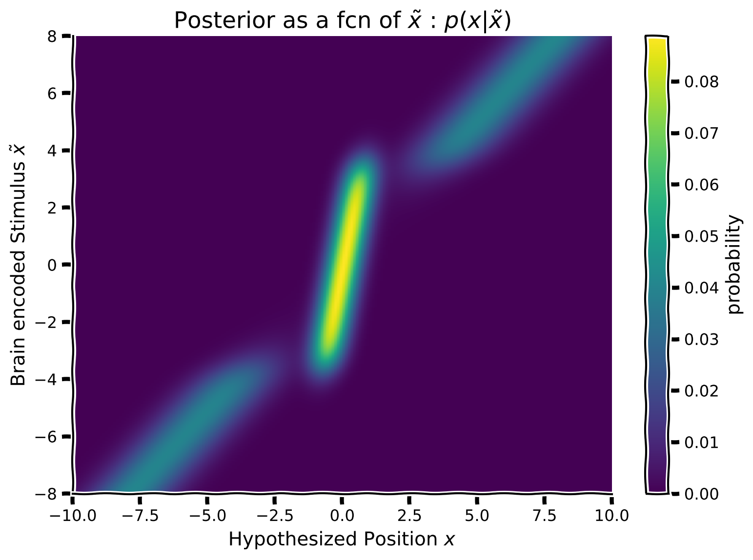
content_review(f"{feedback_prefix}_Posterior_array_Video")

次に、ベイズ則を使って事後分布を計算したいと思います。すでに各脳内符号化位置 $\tilde x$ に対して尤度と事前分布を作成しているので、あとはそれらを行ごとに掛け合わせるだけです。つまり、事後分布配列の各行は、同じ行番号の事前分布と尤度の積によって得られる事後分布となります。

数学的には：

Posterior\left[i, :\right] \propto Likelihood\left[i, :\right] \odot Prior\left[i, :\right]

ここで $\odot$ は対応する事前分布と尤度の行ベクトル i のアダマール積（要素ごとの積）を表します。

脳内符号化刺激 $\tilde x$ の関数として事後分布を構築するために、以下の手順に従ってください：

事前分布と尤度の各行（すなわち各脳内符号化 $\tilde x$ ）について、事後分布行列を埋めていきます。事後分布配列の各行は異なる脳内符号化 $\tilde x$ に対する事後密度を表すようにします。
すでにスクリプト内にコメントアウトされている関数 $plot_myarray()$ を使って配列をプロットしてください。

オプション：

1つの要素や1行ずつ処理する必要がありますか？NumPyの操作はしばしば行列全体を一度に「ベクトル化」して処理できます。この方法は要素ごとの計算よりも高速で読みやすいことが多いです。forループを使わずに事後分布を計算するベクトル化バージョンを書いてみましょう。ヒント: np.sum とそのキーワード引数を参照してください。

コーディング演習 3: 仮想刺激 $x$ の関数として事後分布を計算する

def calculate_posterior_array(prior_array, likelihood_array):
  ############################################################################
  ## Insert your code here to:
  ##      - calculate the 'posterior_array' from the given
  ##        'prior_array', 'likelihood_array'
  ##      - normalize
  ## remove the raise below to test your function
  raise NotImplementedError("You need to complete the function!")
  ############################################################################
  posterior_array = ...
  posterior_array /= ...  # normalize each row separately

  return posterior_array


posterior_array = calculate_posterior_array(prior_array, likelihood_array)
plot_myarray(posterior_array,
             'Hypothesized Position $x$',
             'Brain encoded Stimulus $\~x$',
             'Posterior as a fcn of $\~x$ : $p(x | \~x)$')

解答を見る$

出力例:

# @title Submit your feedback
content_review(f"{feedback_prefix}_Calculate_posterior_Exercise")

セクション 4: 位置 $\hat x$ の推定

# @title Video 4: Binary decision matrix
from ipywidgets import widgets
from IPython.display import YouTubeVideo
from IPython.display import IFrame
from IPython.display import display


class PlayVideo(IFrame):
  def __init__(self, id, source, page=1, width=400, height=300, **kwargs):
    self.id = id
    if source == 'Bilibili':
      src = f'https://player.bilibili.com/player.html?bvid={id}&page={page}'
    elif source == 'Osf':
      src = f'https://mfr.ca-1.osf.io/render?url=https://osf.io/download/{id}/?direct%26mode=render'
    super(PlayVideo, self).__init__(src, width, height, **kwargs)


def display_videos(video_ids, W=400, H=300, fs=1):
  tab_contents = []
  for i, video_id in enumerate(video_ids):
    out = widgets.Output()
    with out:
      if video_ids[i][0] == 'Youtube':
        video = YouTubeVideo(id=video_ids[i][1], width=W,
                             height=H, fs=fs, rel=0)
        print(f'Video available at https://youtube.com/watch?v={video.id}')
      else:
        video = PlayVideo(id=video_ids[i][1], source=video_ids[i][0], width=W,
                          height=H, fs=fs, autoplay=False)
        if video_ids[i][0] == 'Bilibili':
          print(f'Video available at https://www.bilibili.com/video/{video.id}')
        elif video_ids[i][0] == 'Osf':
          print(f'Video available at https://osf.io/{video.id}')
      display(video)
    tab_contents.append(out)
  return tab_contents


video_ids = [('Youtube', 'gy3GmlssHgQ'), ('Bilibili', 'BV1sZ4y1u74e')]
tab_contents = display_videos(video_ids, W=854, H=480)
tabs = widgets.Tab()
tabs.children = tab_contents
for i in range(len(tab_contents)):
  tabs.set_title(i, video_ids[i][0])
display(tabs)

# @title Submit your feedback
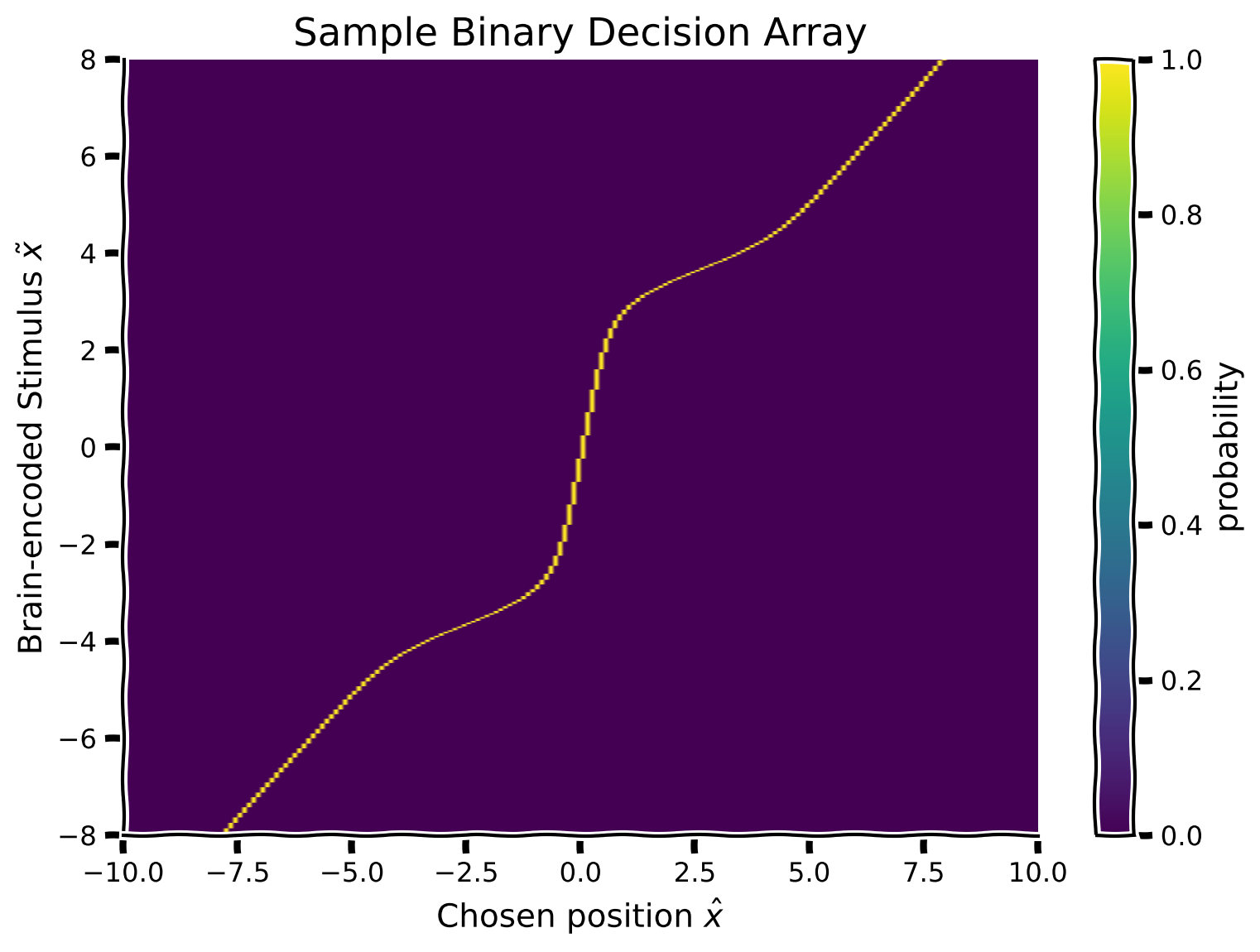
content_review(f"{feedback_prefix}_Binary_decision_matrix_Video")

脳の推定刺激位置を表す事後分布（各可能な脳の符号化 $\tilde x$ に対して） $p(x|\tilde x)$ が得られたので、この事後分布を用いて音源位置 $\hat x$ の推定（応答）を行いたいと思います。これは、被験者の（実験者である私たちには観測不可能な）脳の符号化が各可能な値を取った場合の推定を表します。

これは実質的に、参加者がある脳の符号化 $\tilde x$ に対して行う意思決定を符号化しています。この演習では、参加者が事後分布の平均（決定規則）を音源位置の推定応答として取ると仮定します（事後分布の平均を計算するために、提供されている関数 $moments_myfunc()$ を使用してください）。

この知識を用いて、 $\hat x$ を符号化された刺激 $\tilde x$ の関数として表現します。これにより、2次元のバイナリ意思決定配列が得られます。そのために、事後分布の行列（行方向）を走査し、行ごとの事後分布の平均の位置に対応する配列のセルの値を1に設定します。

提案

各脳の符号化 $\tilde x$ （事後配列の各行）について、事後分布の平均を計算し、対応するバイナリ意思決定配列のセルを1に設定してください（例：事後分布の平均が位置0なら、x_column == 0 のセルを1に設定）。
既にスクリプト内にコメントアウトされている関数 $plot_myarray()$ を使って行列をプロットしてください

コーディング演習4: 仮想刺激 $x$ の関数として推定応答を計算する

def calculate_binary_decision_array(x_points, posterior_array):

  binary_decision_array = np.zeros_like(posterior_array)

  for i in range(len(posterior_array)):
    ########################################################################
    ## Insert your code here to:
    ##      - For each hypothetical stimulus x (row of posterior),
    ##        calculate the mean of the posterior using the provided function
    ##        `moments_myfunc()`, and set the corresponding cell of the
    ##        Binary Decision array to 1.
    ##        Hint: you can run 'help(moments_myfunc)' to see the docstring
    ## remove the raise below to test your function
    raise NotImplementedError("You need to complete the function!")
    ########################################################################
    # calculate mean of posterior using 'moments_myfunc'
    mean, _, _ = ...
    # find the position of mean in x_points (closest position)
    idx = ...
    binary_decision_array[i, idx] = 1

  return binary_decision_array


binary_decision_array = calculate_binary_decision_array(x, posterior_array)
plot_myarray(binary_decision_array,
             'Chosen position $\hat x$', 'Brain-encoded Stimulus $\~ x$',
             'Sample Binary Decision Array')

解答を見る$

出力例:

# @title Submit your feedback
content_review(f"{feedback_prefix}_Calculate_estimated_response_Exercise")

セクション5: 符号化された刺激の確率

# @title Video 5: Input array
from ipywidgets import widgets
from IPython.display import YouTubeVideo
from IPython.display import IFrame
from IPython.display import display


class PlayVideo(IFrame):
  def __init__(self, id, source, page=1, width=400, height=300, **kwargs):
    self.id = id
    if source == 'Bilibili':
      src = f'https://player.bilibili.com/player.html?bvid={id}&page={page}'
    elif source == 'Osf':
      src = f'https://mfr.ca-1.osf.io/render?url=https://osf.io/download/{id}/?direct%26mode=render'
    super(PlayVideo, self).__init__(src, width, height, **kwargs)


def display_videos(video_ids, W=400, H=300, fs=1):
  tab_contents = []
  for i, video_id in enumerate(video_ids):
    out = widgets.Output()
    with out:
      if video_ids[i][0] == 'Youtube':
        video = YouTubeVideo(id=video_ids[i][1], width=W,
                             height=H, fs=fs, rel=0)
        print(f'Video available at https://youtube.com/watch?v={video.id}')
      else:
        video = PlayVideo(id=video_ids[i][1], source=video_ids[i][0], width=W,
                          height=H, fs=fs, autoplay=False)
        if video_ids[i][0] == 'Bilibili':
          print(f'Video available at https://www.bilibili.com/video/{video.id}')
        elif video_ids[i][0] == 'Osf':
          print(f'Video available at https://osf.io/{video.id}')
      display(video)
    tab_contents.append(out)
  return tab_contents


video_ids = [('Youtube', 'C1d1n_Si83o'), ('Bilibili', 'BV1pT4y1E7wv')]
tab_contents = display_videos(video_ids, W=854, H=480)
tabs = widgets.Tab()
tabs.children = tab_contents
for i in range(len(tab_contents)):
  tabs.set_title(i, video_ids[i][0])
display(tabs)

# @title Submit your feedback
content_review(f"{feedback_prefix}_Input_array_Video")

私たち実験者は、既知の刺激 $x$ に対する符号化 $\tilde x$ を知ることができないため、各可能な符号化に対してバイナリ意思決定配列を計算する必要がありました。

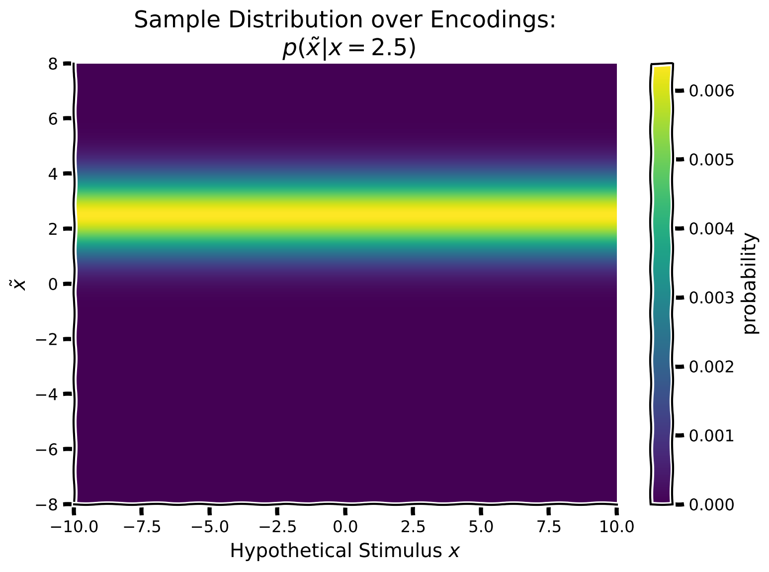
しかしまず、真の刺激に対して各可能な符号化がどれほど起こりやすいかを計算する必要があります。つまり、真の提示刺激を中心としたガウス分布（ $\sigma = 1$ ）を作成し、これを潜在的な符号化値 $\tilde x$ の関数として繰り返します。具体的には、真の提示刺激を中心とした列方向のガウス分布を作成し、この列ガウスをすべての仮想刺激値 $x$ にわたって繰り返します。

これは、脳が符号化した刺激の分布（私たち実験者が知っている単一の刺激）を実質的に符号化し、真の刺激 $x$ と潜在的な符号化 $\tilde x$ を結びつけることを可能にします。

提案

この演習では、真の刺激が方向2.5で提示されたと仮定します。

平均 $\mu = 2.5$ 、標準偏差 $\sigma = 1.0$ のガウス尤度を作成してください
これを配列の最初の列とし、その列を繰り返して仮想刺激位置の関数として真の提示刺激入力を埋めてください
既にスクリプト内にコメントアウトされている関数 $plot_myarray()$ を使って配列をプロットしてください

コーディング演習5: 仮想刺激 $x$ の関数として入力を生成する

def generate_input_array(x_points, stim_array, posterior_array,
                         mean=2.5, sigma=1.):

  input_array = np.zeros_like(posterior_array)
  ########################################################################
  ## Insert your code here to:
  ##      - Generate a gaussian centered on the true stimulus 2.5
  ##        and sigma = 1. for each column
  ## remove the raise below to test your function
  raise NotImplementedError("You need to complete the function!")
  ########################################################################
  for i in range(len(x_points)):
    input_array[:, i] = ...

  return input_array


input_array = generate_input_array(x, hypothetical_stim, posterior_array)
plot_myarray(input_array,
             'Hypothetical Stimulus $x$', '$\~x$',
             'Sample Distribution over Encodings:\n $p(\~x | x = 2.5)$')

解答を見る$

出力例:

# @title Submit your feedback
content_review(f"{feedback_prefix}_Generate_input_array_Exercise")

セクション6: 正規化と期待推定分布

# @title Video 6: Marginalization
from ipywidgets import widgets
from IPython.display import YouTubeVideo
from IPython.display import IFrame
from IPython.display import display


class PlayVideo(IFrame):
  def __init__(self, id, source, page=1, width=400, height=300, **kwargs):
    self.id = id
    if source == 'Bilibili':
      src = f'https://player.bilibili.com/player.html?bvid={id}&page={page}'
    elif source == 'Osf':
      src = f'https://mfr.ca-1.osf.io/render?url=https://osf.io/download/{id}/?direct%26mode=render'
    super(PlayVideo, self).__init__(src, width, height, **kwargs)


def display_videos(video_ids, W=400, H=300, fs=1):
  tab_contents = []
  for i, video_id in enumerate(video_ids):
    out = widgets.Output()
    with out:
      if video_ids[i][0] == 'Youtube':
        video = YouTubeVideo(id=video_ids[i][1], width=W,
                             height=H, fs=fs, rel=0)
        print(f'Video available at https://youtube.com/watch?v={video.id}')
      else:
        video = PlayVideo(id=video_ids[i][1], source=video_ids[i][0], width=W,
                          height=H, fs=fs, autoplay=False)
        if video_ids[i][0] == 'Bilibili':
          print(f'Video available at https://www.bilibili.com/video/{video.id}')
        elif video_ids[i][0] == 'Osf':
          print(f'Video available at https://osf.io/{video.id}')
      display(video)
    tab_contents.append(out)
  return tab_contents


video_ids = [('Youtube', '5alwtNS4CGw'), ('Bilibili', 'BV1qz4y1D71K')]
tab_contents = display_videos(video_ids, W=854, H=480)
tabs = widgets.Tab()
tabs.children = tab_contents
for i in range(len(tab_contents)):
  tabs.set_title(i, video_ids[i][0])
display(tabs)

# @title Submit your feedback
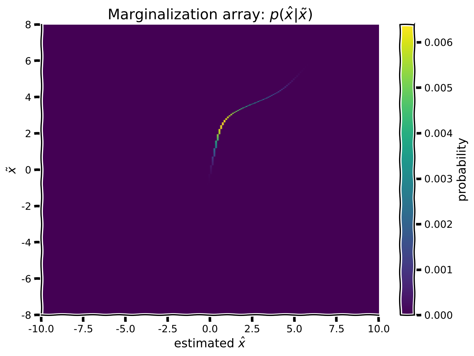
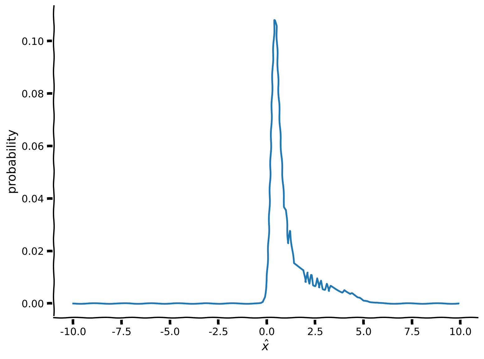
content_review(f"{feedback_prefix}_Marginalization_Video")

真の刺激 $x$ とそれを潜在的な符号化に結びつける方法が得られたので、符号化の分布と最終的な推定の分布を計算できるようになります。すべての可能な $\tilde x$ の値にわたって積分（周辺化）するために、真の提示刺激とバイナリ意思決定配列のドット積を計算し、その後 $x$ にわたって和を取ります。

数学的には、以下を計算したいということです。

\begin{eqnarray}
$\text{周辺化配列} = \text{入力配列} \odot \text{バイナリ意思決定配列}
\end{eqnarray}

\begin{eqnarray}
\text{周辺化} = \int_{\tilde x} \text{周辺化配列}
\end{eqnarray}$

離散値に対して配列を用いて積分を行うため、積分は単純に $\tilde x$ にわたる和に帰着します。

提案

入力配列とバイナリ配列の各行について積を計算し、2次元の周辺化配列に埋めてください
既にスクリプト内にコメントアウトされている関数 $plot_myarray()$ を使って結果をプロットしてください
スクリプト内にコメントアウトされているコードスニペットを使い、 $x$ $x$ にわたる周辺化を計算・プロットしてください
- 数値積分の制限により、周辺化にアーティファクトが生じることに注意してください

コーディング演習 6: 周辺化行列の実装

def my_marginalization(input_array, binary_decision_array):

  ############################################################################
  ## Insert your code here to:
  ##  - Compute 'marginalization_array' by multiplying pointwise the Binary
  ##    decision array over hypothetical stimuli and the Input array
  ##  - Compute 'marginal' from the 'marginalization_array' by summing over x
  ##    (hint: use np.sum() and only marginalize along the columns)
  ## remove the raise below to test your function
  raise NotImplementedError("You need to complete the function!")
  ############################################################################

  marginalization_array = ...
  marginal = ... # note axis
  marginal /= ... # normalize

  return marginalization_array, marginal


marginalization_array, marginal = my_marginalization(input_array, binary_decision_array)

plot_myarray(marginalization_array,
             'estimated $\hat x$',
             '$\~x$',
             'Marginalization array: $p(\^x | \~x)$')
plt.figure()
plt.plot(x, marginal)
plt.xlabel('$\^x$')
plt.ylabel('probability')
plt.show()

解答を見る$

出力例:

# @title Submit your feedback
content_review(f"{feedback_prefix}_Implement_marginalization_matrix_Exercise")

データの生成

事後分布を計算し、 $\tilde x$ を周辺化して $p(\hat{x} \mid x)$ を得る方法を見てきました。次に、提供された $generate_data()$ 関数を使って、単一の参加者の人工データを生成します。混合パラメータは $p_{independent} = 0.1$ とします。

次の演習の目標は、このパラメータを復元することです。パラメータ復元実験は、ベイズ解析の計画やデバッグに非常に有効な方法です。もし与えられたパラメータを復元できなければ、どこかに問題があるということです！なお、この $p_{independent}$ の値は、事前分布で用いた $p_{independent} = 0.05$ とは異なります。これにより、完全なモデルの検証が可能になります。

以下のコードを実行して合成データを生成してください。編集は不要ですが、下のプロットが動画の内容と一致しているか確認してください。

#@title
#@markdown #### Run the 'generate_data' function (this cell)
def generate_data(x_stim, p_independent):
  """
  DO NOT EDIT THIS FUNCTION !!!

  Returns generated data using the mixture of Gaussian prior with mixture
  parameter `p_independent`

  Args :
    x_stim (numpy array of floats) - x values at which stimuli are presented
    p_independent (scalar) - mixture component for the Mixture of Gaussian prior

  Returns:
    (numpy array of floats): x_hat response of participant for each stimulus
  """
  x = np.arange(-10,10,0.1)
  x_hat = np.zeros_like(x_stim)

  prior_mean = 0
  prior_sigma1 = .5
  prior_sigma2 = 3
  prior1 = my_gaussian(x, prior_mean, prior_sigma1)
  prior2 = my_gaussian(x, prior_mean, prior_sigma2)

  prior_combined = (1-p_independent) * prior1 + (p_independent * prior2)
  prior_combined = prior_combined / np.sum(prior_combined)

  for i_stim in np.arange(x_stim.shape[0]):
    likelihood_mean = x_stim[i_stim]
    likelihood_sigma  = 1
    likelihood = my_gaussian(x, likelihood_mean, likelihood_sigma)
    likelihood = likelihood / np.sum(likelihood)

    posterior = np.multiply(prior_combined, likelihood)
    posterior = posterior / np.sum(posterior)

    # Assumes participant takes posterior mean as 'action'
    x_hat[i_stim] = np.sum(x * posterior)
  return x_hat

# Generate data for a single participant
true_stim = np.array([-8, -4, -3, -2.5, -2, -1.5, -1, -0.5, 0, 0.5, 1, 1.5, 2,
                      2.5, 3, 4, 8])
behaviour = generate_data(true_stim, 0.10)

plot_simulated_behavior(true_stim, behaviour)

セクション7: モデルフィッティング

# @title Video 7: Log likelihood
from ipywidgets import widgets
from IPython.display import YouTubeVideo
from IPython.display import IFrame
from IPython.display import display


class PlayVideo(IFrame):
  def __init__(self, id, source, page=1, width=400, height=300, **kwargs):
    self.id = id
    if source == 'Bilibili':
      src = f'https://player.bilibili.com/player.html?bvid={id}&page={page}'
    elif source == 'Osf':
      src = f'https://mfr.ca-1.osf.io/render?url=https://osf.io/download/{id}/?direct%26mode=render'
    super(PlayVideo, self).__init__(src, width, height, **kwargs)


def display_videos(video_ids, W=400, H=300, fs=1):
  tab_contents = []
  for i, video_id in enumerate(video_ids):
    out = widgets.Output()
    with out:
      if video_ids[i][0] == 'Youtube':
        video = YouTubeVideo(id=video_ids[i][1], width=W,
                             height=H, fs=fs, rel=0)
        print(f'Video available at https://youtube.com/watch?v={video.id}')
      else:
        video = PlayVideo(id=video_ids[i][1], source=video_ids[i][0], width=W,
                          height=H, fs=fs, autoplay=False)
        if video_ids[i][0] == 'Bilibili':
          print(f'Video available at https://www.bilibili.com/video/{video.id}')
        elif video_ids[i][0] == 'Osf':
          print(f'Video available at https://osf.io/{video.id}')
      display(video)
    tab_contents.append(out)
  return tab_contents


video_ids = [('Youtube', 'jbYauFpyZhs'), ('Bilibili', 'BV1Yf4y1R7ST')]
tab_contents = display_videos(video_ids, W=854, H=480)
tabs = widgets.Tab()
tabs.children = tab_contents
for i in range(len(tab_contents)):
  tabs.set_title(i, video_ids[i][0])
display(tabs)

# @title Submit your feedback
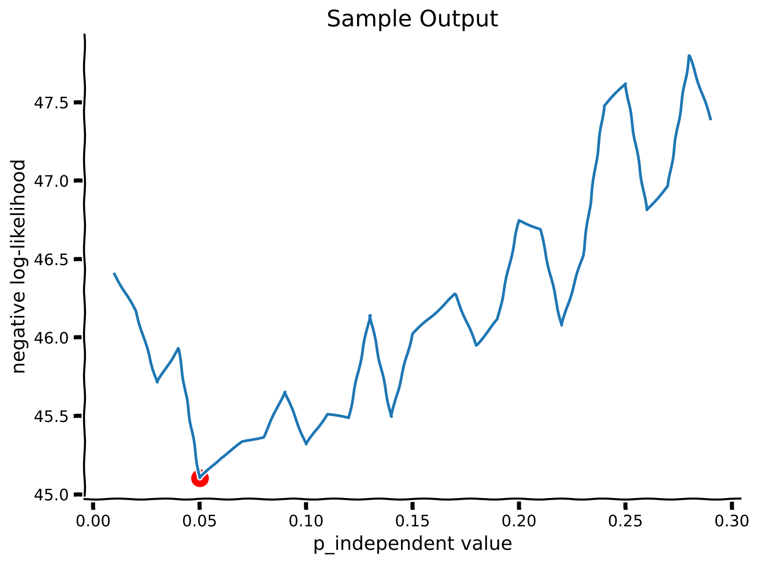
content_review(f"{feedback_prefix}_Loglikelihood_Video")

データを生成したので、次にそのデータを生成するために使われたパラメータ $p_{independent}$ を推定してみましょう。

未完成の関数 $my_Bayes_model_mse()$ が用意されています。この関数を完成させて、これまでの演習で行った計算を、単一の試行ではなく全ての参加者の試行に対して実行できるようにしてください。

尤度はすでに構築されています。これは仮定された刺激にのみ依存するため変わりません。しかし、 $p_{independent}$ に依存する事前分布の行列は実装する必要があります。したがって、事後分布、入力、周辺化を再計算して $p(\hat{x} \mid x)$ を得る必要があります。

得られた $p(\hat{x} \mid x)$ を用いて、各試行の負の対数尤度を計算し、負の対数尤度を最小化する（すなわち対数尤度を最大化する） $p_{independent}$ の値を見つけます。復習のために、モデルフィッティングのチュートリアル$ を参照してください。

この実験では、試行は互いに独立であると仮定します。これは一般的な仮定であり、しばしば正しいこともあります。これにより、負の対数尤度を以下のように定義できます：

-LL = - \sum_i \log p(\hat{x}_i \mid x_i)

ここで、 $\hat{x}_i$ は試行 $i$ における参加者の応答、 $x_i$ は提示された刺激です。

関数 my_Bayes_model_mse を完成させてください。事前分布、事後分布、入力の配列はすでに各試行で計算されるように準備されています。
周辺化配列および各試行での周辺化を計算してください。
周辺化と参加者の応答を用いて負の対数尤度を計算してください。
スクリプト内でコメントアウトされているコードスニペットを使い、可能な $p_{independent}$ の値をループ処理してください。

コーディング演習 7: 生成データへのモデルフィッティング

def my_Bayes_model_mse(params):
  """
  Function fits the Bayesian model from Tutorial 4

  Args :
      params (list of positive floats):  parameters used by the model
      (params[0]  = posterior scaling)

  Returns :
      (scalar) negative log-likelihood :sum of log probabilities
  """
  # Create the prior array
  p_independent=params[0]
  prior_array = calculate_prior_array(x,
                                      hypothetical_stim,
                                      p_independent,
                                      prior_sigma_indep= 3.)
  # Create posterior array
  posterior_array = calculate_posterior_array(prior_array, likelihood_array)
  # Create Binary decision array
  binary_decision_array = calculate_binary_decision_array(x, posterior_array)
  # we will use trial_ll (trial log likelihood) to register each trial
  trial_ll = np.zeros_like(true_stim)

  # Loop over stimuli
  for i_stim in range(len(true_stim)):
    # create the input array with true_stim as mean
    input_array = np.zeros_like(posterior_array)
    for i in range(len(x)):
      input_array[:, i] = my_gaussian(hypothetical_stim, true_stim[i_stim], 1)
      input_array[:, i] = input_array[:, i] / np.sum(input_array[:, i])

    # calculate the marginalizations
    marginalization_array, marginal = my_marginalization(input_array,
                                                         binary_decision_array)
    action = behaviour[i_stim]
    idx = np.argmin(np.abs(x - action))
    ########################################################################
    ## Insert your code here to:
    ##      - Compute the log likelihood of the participant
    ## remove the raise below to test your function
    raise NotImplementedError("You need to complete the function!")
    ########################################################################
    # Get the marginal likelihood corresponding to the action
    marginal_nonzero = ... + np.finfo(float).eps  # avoid log(0)
    trial_ll[i_stim] = np.log(marginal_nonzero)

  neg_ll = -trial_ll.sum()

  return neg_ll


plot_my_bayes_model(my_Bayes_model_mse)

解答を見る$

出力例:

# @title Submit your feedback
content_review(f"{feedback_prefix}_Fitting_a_model_to_generated_data_Exercise")

セクション 8: まとめ

# @title Video 8: Outro
from ipywidgets import widgets
from IPython.display import YouTubeVideo
from IPython.display import IFrame
from IPython.display import display


class PlayVideo(IFrame):
  def __init__(self, id, source, page=1, width=400, height=300, **kwargs):
    self.id = id
    if source == 'Bilibili':
      src = f'https://player.bilibili.com/player.html?bvid={id}&page={page}'
    elif source == 'Osf':
      src = f'https://mfr.ca-1.osf.io/render?url=https://osf.io/download/{id}/?direct%26mode=render'
    super(PlayVideo, self).__init__(src, width, height, **kwargs)


def display_videos(video_ids, W=400, H=300, fs=1):
  tab_contents = []
  for i, video_id in enumerate(video_ids):
    out = widgets.Output()
    with out:
      if video_ids[i][0] == 'Youtube':
        video = YouTubeVideo(id=video_ids[i][1], width=W,
                             height=H, fs=fs, rel=0)
        print(f'Video available at https://youtube.com/watch?v={video.id}')
      else:
        video = PlayVideo(id=video_ids[i][1], source=video_ids[i][0], width=W,
                          height=H, fs=fs, autoplay=False)
        if video_ids[i][0] == 'Bilibili':
          print(f'Video available at https://www.bilibili.com/video/{video.id}')
        elif video_ids[i][0] == 'Osf':
          print(f'Video available at https://osf.io/{video.id}')
      display(video)
    tab_contents.append(out)
  return tab_contents


video_ids = [('Youtube', 'F5JfqJonz20'), ('Bilibili', 'BV1Hz411v7hJ')]
tab_contents = display_videos(video_ids, W=854, H=480)
tabs = widgets.Tab()
tabs.children = tab_contents
for i in range(len(tab_contents)):
  tabs.set_title(i, video_ids[i][0])
display(tabs)

# @title Submit your feedback
content_review(f"{feedback_prefix}_Outro_Video")

おめでとうございます！ $p_{independent}$ 、つまり被験者が音の同一原因起源と独立原因起源にどれだけの重みを割り当てるかを表すパラメータを見つけました。これまでのノートブックでは、ベイズ解析の全プロセスを通して学びました：

モデルの構築
データのシミュレーション
ベイズの定理と周辺化を用いてデータから隠れたパラメータを推定する

この例はシンプルでしたが、同じ原理は多くの隠れ変数や複雑な事前分布・尤度を持つデータセットの解析にも応用できます。

ボーナスチュートリアル: データへのフィッティング

チュートリアルの目的

セットアップ

はじめに

セクション1: 尤度配列

コーディング演習1: 真の刺激位置の関数として聴覚尤度を実装する

セクション 2: ガウス事前分布の因果混合

コーディング演習 2: 事前配列の実装

セクション3: ベイズの定理と事後分布配列

コーディング演習 3: 仮想刺激 xxx の関数として事後分布を計算する

セクション 4: 位置 x^\hat xx^ の推定

コーディング演習4: 仮想刺激 xxx の関数として推定応答を計算する

セクション5: 符号化された刺激の確率

コーディング演習5: 仮想刺激 xxx の関数として入力を生成する

セクション6: 正規化と期待推定分布

コーディング演習 6: 周辺化行列の実装

データの生成

セクション7: モデルフィッティング

コーディング演習 7: 生成データへのモデルフィッティング

セクション 8: まとめ

コーディング演習 3: 仮想刺激 $x$ の関数として事後分布を計算する

セクション 4: 位置 $\hat x$ の推定

コーディング演習4: 仮想刺激 $x$ の関数として推定応答を計算する

コーディング演習5: 仮想刺激 $x$ の関数として入力を生成する