ボーナスチュートリアル: Wilson-Cowanモデルの拡張

第2週、第5日目: 動的ネットワーク

Neuromatch Academyによる

コンテンツ制作者: Qinglong Gu, Songtin Li, Arvind Kumar, John Murray, Julijana Gjorgjieva

コンテンツレビュアー: Maryam Vaziri-Pashkam, Ella Batty, Lorenzo Fontolan, Richard Gao, Spiros Chavlis, Michael Waskom

制作編集者: Siddharth Suresh, Gagana B, Spiros Chavlis

チュートリアルの目的

前回のチュートリアルでは、Wilson-Cowan レートモデルについて学びました。ここでは、このモデルのより深い解析に踏み込みます。

ボーナスステップ:

Wilson-Cowanモデルの固定点を見つけてプロットする。
動力学を線形化し、ヤコビ行列を調べることでWilson-Cowanモデルの安定性を調査する。
Wilson-Cowanモデルがどのようにして振動状態に到達するかを学ぶ。

Wilson-Cowanモデルの応用:

抑制安定化ネットワークの挙動を可視化する。
Wilson-Cowanモデルを用いて作業記憶をシミュレートする。

参考文献:

Wilson, H., and Cowan, J. (1972). Excitatory and inhibitory interactions in localized populations of model neurons. Biophysical Journal 12. doi: 10.1016/S0006-3495(72)86068-5

セットアップ

# @title Install and import feedback gadget


from vibecheck import DatatopsContentReviewContainer
def content_review(notebook_section: str):
    return DatatopsContentReviewContainer(
        "",  # No text prompt
        notebook_section,
        {
            "url": "https://pmyvdlilci.execute-api.us-east-1.amazonaws.com/klab",
            "name": "neuromatch_cn",
            "user_key": "y1x3mpx5",
        },
    ).render()


feedback_prefix = "W2D4_T3_Bonus"

# Imports
import matplotlib.pyplot as plt
import numpy as np
import scipy.optimize as opt  # root-finding algorithm

# @title Figure Settings
import logging
logging.getLogger('matplotlib.font_manager').disabled = True

import ipywidgets as widgets  # interactive display
%config InlineBackend.figure_format = 'retina'
plt.style.use("https://raw.githubusercontent.com/NeuromatchAcademy/course-content/main/nma.mplstyle")

# @title Plotting Functions

def plot_FI_inverse(x, a, theta):
  f, ax = plt.subplots()
  ax.plot(x, F_inv(x, a=a, theta=theta))
  ax.set(xlabel="$x$", ylabel="$F^{-1}(x)$")


def plot_FI_EI(x, FI_exc, FI_inh):
  plt.figure()
  plt.plot(x, FI_exc, 'b', label='E population')
  plt.plot(x, FI_inh, 'r', label='I population')
  plt.legend(loc='lower right')
  plt.xlabel('x (a.u.)')
  plt.ylabel('F(x)')
  plt.show()


def my_test_plot(t, rE1, rI1, rE2, rI2):

  plt.figure()
  ax1 = plt.subplot(211)
  ax1.plot(pars['range_t'], rE1, 'b', label='E population')
  ax1.plot(pars['range_t'], rI1, 'r', label='I population')
  ax1.set_ylabel('Activity')
  ax1.legend(loc='best')

  ax2 = plt.subplot(212, sharex=ax1, sharey=ax1)
  ax2.plot(pars['range_t'], rE2, 'b', label='E population')
  ax2.plot(pars['range_t'], rI2, 'r', label='I population')
  ax2.set_xlabel('t (ms)')
  ax2.set_ylabel('Activity')
  ax2.legend(loc='best')

  plt.tight_layout()
  plt.show()


def plot_nullclines(Exc_null_rE, Exc_null_rI, Inh_null_rE, Inh_null_rI):

  plt.figure()
  plt.plot(Exc_null_rE, Exc_null_rI, 'b', label='E nullcline')
  plt.plot(Inh_null_rE, Inh_null_rI, 'r', label='I nullcline')
  plt.xlabel(r'$r_E$')
  plt.ylabel(r'$r_I$')
  plt.legend(loc='best')
  plt.show()


def my_plot_nullcline(pars):
  Exc_null_rE = np.linspace(-0.01, 0.96, 100)
  Exc_null_rI = get_E_nullcline(Exc_null_rE, **pars)
  Inh_null_rI = np.linspace(-.01, 0.8, 100)
  Inh_null_rE = get_I_nullcline(Inh_null_rI, **pars)

  plt.plot(Exc_null_rE, Exc_null_rI, 'b', label='E nullcline')
  plt.plot(Inh_null_rE, Inh_null_rI, 'r', label='I nullcline')
  plt.xlabel(r'$r_E$')
  plt.ylabel(r'$r_I$')
  plt.legend(loc='best')


def my_plot_vector(pars, my_n_skip=2, myscale=5):
  EI_grid = np.linspace(0., 1., 20)
  rE, rI = np.meshgrid(EI_grid, EI_grid)
  drEdt, drIdt = EIderivs(rE, rI, **pars)

  n_skip = my_n_skip

  plt.quiver(rE[::n_skip, ::n_skip], rI[::n_skip, ::n_skip],
             drEdt[::n_skip, ::n_skip], drIdt[::n_skip, ::n_skip],
             angles='xy', scale_units='xy', scale=myscale, facecolor='c')

  plt.xlabel(r'$r_E$')
  plt.ylabel(r'$r_I$')


def my_plot_trajectory(pars, mycolor, x_init, mylabel):
  pars = pars.copy()
  pars['rE_init'], pars['rI_init'] = x_init[0], x_init[1]
  rE_tj, rI_tj = simulate_wc(**pars)

  plt.plot(rE_tj, rI_tj, color=mycolor, label=mylabel)
  plt.plot(x_init[0], x_init[1], 'o', color=mycolor, ms=8)
  plt.xlabel(r'$r_E$')
  plt.ylabel(r'$r_I$')


def my_plot_trajectories(pars, dx, n, mylabel):
  """
  Solve for I along the E_grid from dE/dt = 0.

  Expects:
  pars    : Parameter dictionary
  dx      : increment of initial values
  n       : n*n trjectories
  mylabel : label for legend

  Returns:
    figure of trajectory
  """
  pars = pars.copy()
  for ie in range(n):
    for ii in range(n):
      pars['rE_init'], pars['rI_init'] = dx * ie, dx * ii
      rE_tj, rI_tj = simulate_wc(**pars)
      if (ie == n-1) & (ii == n-1):
          plt.plot(rE_tj, rI_tj, 'gray', alpha=0.8, label=mylabel)
      else:
          plt.plot(rE_tj, rI_tj, 'gray', alpha=0.8)

  plt.xlabel(r'$r_E$')
  plt.ylabel(r'$r_I$')


def plot_complete_analysis(pars):
  plt.figure(figsize=(7.7, 6.))

  # plot example trajectories
  my_plot_trajectories(pars, 0.2, 6,
                       'Sample trajectories \nfor different init. conditions')
  my_plot_trajectory(pars, 'orange', [0.6, 0.8],
                     'Sample trajectory for \nlow activity')
  my_plot_trajectory(pars, 'm', [0.6, 0.6],
                     'Sample trajectory for \nhigh activity')

  # plot nullclines
  my_plot_nullcline(pars)

  # plot vector field
  EI_grid = np.linspace(0., 1., 20)
  rE, rI = np.meshgrid(EI_grid, EI_grid)
  drEdt, drIdt = EIderivs(rE, rI, **pars)
  n_skip = 2
  plt.quiver(rE[::n_skip, ::n_skip], rI[::n_skip, ::n_skip],
             drEdt[::n_skip, ::n_skip], drIdt[::n_skip, ::n_skip],
             angles='xy', scale_units='xy', scale=5., facecolor='c')

  plt.legend(loc=[1.02, 0.57], handlelength=1)
  plt.show()


def plot_fp(x_fp, position=(0.02, 0.1), rotation=0):
  plt.plot(x_fp[0], x_fp[1], 'ko', ms=8)
  plt.text(x_fp[0] + position[0], x_fp[1] + position[1],
           f'Fixed Point1=\n({x_fp[0]:.3f}, {x_fp[1]:.3f})',
           horizontalalignment='center', verticalalignment='bottom',
           rotation=rotation)

# @title Helper functions


def default_pars(**kwargs):
  pars = {}

  # Excitatory parameters
  pars['tau_E'] = 1.     # Timescale of the E population [ms]
  pars['a_E'] = 1.2      # Gain of the E population
  pars['theta_E'] = 2.8  # Threshold of the E population

  # Inhibitory parameters
  pars['tau_I'] = 2.0    # Timescale of the I population [ms]
  pars['a_I'] = 1.0      # Gain of the I population
  pars['theta_I'] = 4.0  # Threshold of the I population

  # Connection strength
  pars['wEE'] = 9.   # E to E
  pars['wEI'] = 4.   # I to E
  pars['wIE'] = 13.  # E to I
  pars['wII'] = 11.  # I to I

  # External input
  pars['I_ext_E'] = 0.
  pars['I_ext_I'] = 0.

  # simulation parameters
  pars['T'] = 50.        # Total duration of simulation [ms]
  pars['dt'] = .1        # Simulation time step [ms]
  pars['rE_init'] = 0.2  # Initial value of E
  pars['rI_init'] = 0.2  # Initial value of I

  # External parameters if any
  for k in kwargs:
      pars[k] = kwargs[k]

  # Vector of discretized time points [ms]
  pars['range_t'] = np.arange(0, pars['T'], pars['dt'])

  return pars


def F(x, a, theta):
  """
  Population activation function, F-I curve

  Args:
    x     : the population input
    a     : the gain of the function
    theta : the threshold of the function

  Returns:
    f     : the population activation response f(x) for input x
  """

  # add the expression of f = F(x)
  f = (1 + np.exp(-a * (x - theta)))**-1 - (1 + np.exp(a * theta))**-1

  return f


def dF(x, a, theta):
  """
  Derivative of the population activation function.

  Args:
    x     : the population input
    a     : the gain of the function
    theta : the threshold of the function

  Returns:
    dFdx  :  Derivative of the population activation function.
  """

  dFdx = a * np.exp(-a * (x - theta)) * (1 + np.exp(-a * (x - theta)))**-2

  return dFdx

def F_inv(x, a, theta):
  """
  Args:
    x         : the population input
    a         : the gain of the function
    theta     : the threshold of the function

  Returns:
    F_inverse : value of the inverse function
  """

  # Calculate Finverse (ln(x) can be calculated as np.log(x))
  F_inverse = -1/a * np.log((x + (1 + np.exp(a * theta))**-1)**-1 - 1) + theta

  return F_inverse


def get_E_nullcline(rE, a_E, theta_E, wEE, wEI, I_ext_E, **other_pars):
  """
  Solve for rI along the rE from drE/dt = 0.

  Args:
    rE    : response of excitatory population
    a_E, theta_E, wEE, wEI, I_ext_E : Wilson-Cowan excitatory parameters
    Other parameters are ignored

  Returns:
    rI    : values of inhibitory population along the nullcline on the rE
  """
  # calculate rI for E nullclines on rI
  rI = 1 / wEI * (wEE * rE - F_inv(rE, a_E, theta_E) + I_ext_E)

  return rI


def get_I_nullcline(rI, a_I, theta_I, wIE, wII, I_ext_I, **other_pars):
  """
  Solve for E along the rI from dI/dt = 0.

  Args:
    rI    : response of inhibitory population
    a_I, theta_I, wIE, wII, I_ext_I : Wilson-Cowan inhibitory parameters
    Other parameters are ignored

  Returns:
    rE    : values of the excitatory population along the nullcline on the rI
  """
  # calculate rE for I nullclines on rI
  rE = 1 / wIE * (wII * rI + F_inv(rI, a_I, theta_I) - I_ext_I)

  return rE

def EIderivs(rE, rI,
             tau_E, a_E, theta_E, wEE, wEI, I_ext_E,
             tau_I, a_I, theta_I, wIE, wII, I_ext_I,
             **other_pars):
  """Time derivatives for E/I variables (dE/dt, dI/dt)."""

  # Compute the derivative of rE
  drEdt = (-rE + F(wEE * rE - wEI * rI + I_ext_E, a_E, theta_E)) / tau_E

  # Compute the derivative of rI
  drIdt = (-rI + F(wIE * rE - wII * rI + I_ext_I, a_I, theta_I)) / tau_I

  return drEdt, drIdt

def simulate_wc(tau_E, a_E, theta_E, tau_I, a_I, theta_I,
                wEE, wEI, wIE, wII, I_ext_E, I_ext_I,
                rE_init, rI_init, dt, range_t, **other_pars):
  """
  Simulate the Wilson-Cowan equations

  Args:
    Parameters of the Wilson-Cowan model

  Returns:
    rE, rI (arrays) : Activity of excitatory and inhibitory populations
  """
  # Initialize activity arrays
  Lt = range_t.size
  rE = np.append(rE_init, np.zeros(Lt - 1))
  rI = np.append(rI_init, np.zeros(Lt - 1))
  I_ext_E = I_ext_E * np.ones(Lt)
  I_ext_I = I_ext_I * np.ones(Lt)

  # Simulate the Wilson-Cowan equations
  for k in range(Lt - 1):

    # Calculate the derivative of the E population
    drE = dt / tau_E * (-rE[k] + F(wEE * rE[k] - wEI * rI[k] + I_ext_E[k],
                                   a_E, theta_E))

    # Calculate the derivative of the I population
    drI = dt / tau_I * (-rI[k] + F(wIE * rE[k] - wII * rI[k] + I_ext_I[k],
                                   a_I, theta_I))

    # Update using Euler's method
    rE[k + 1] = rE[k] + drE
    rI[k + 1] = rI[k] + drI

  return rE, rI

含まれているヘルパー関数:

パラメータ辞書: $default_pars(**kwargs)$ $d e f a u l t_{p} a r s (* * k w a r g s)$ 。以下のように使えます:
- pars = default_pars() で全パラメータを取得し、print(pars) で確認可能
- pars = default_pars(T=T_sim, dt=time_step) でシミュレーション時間やタイムステップを変更
- pars = default_pars() の後に pars['New_para'] = value で新しいパラメータを追加
- 個別パラメータを受け取る関数には func(**pars) として渡せる
F-I曲線: F(x, a, theta)
F-I曲線の微分: dF(x, a, theta)
F-I曲線の逆関数: $F_inv$
ヌルクライン計算: get_E_nullcline, get_I_nullcline
E/I変数の微分: EIderivs
Wilson-Cowanモデルのシミュレーション: simulate_wc

セクション1: Wilson-Cowanモデルの固定点、安定性解析、リミットサイクル

動画の訂正: これは第2ボーナスチュートリアルの最初の部分であり、第2チュートリアルの最後の部分ではありません

# @title Video 1: Fixed points and their stability
from ipywidgets import widgets
from IPython.display import YouTubeVideo
from IPython.display import IFrame
from IPython.display import display


class PlayVideo(IFrame):
  def __init__(self, id, source, page=1, width=400, height=300, **kwargs):
    self.id = id
    if source == 'Bilibili':
      src = f'https://player.bilibili.com/player.html?bvid={id}&page={page}'
    elif source == 'Osf':
      src = f'https://mfr.ca-1.osf.io/render?url=https://osf.io/download/{id}/?direct%26mode=render'
    super(PlayVideo, self).__init__(src, width, height, **kwargs)


def display_videos(video_ids, W=400, H=300, fs=1):
  tab_contents = []
  for i, video_id in enumerate(video_ids):
    out = widgets.Output()
    with out:
      if video_ids[i][0] == 'Youtube':
        video = YouTubeVideo(id=video_ids[i][1], width=W,
                             height=H, fs=fs, rel=0)
        print(f'Video available at https://youtube.com/watch?v={video.id}')
      else:
        video = PlayVideo(id=video_ids[i][1], source=video_ids[i][0], width=W,
                          height=H, fs=fs, autoplay=False)
        if video_ids[i][0] == 'Bilibili':
          print(f'Video available at https://www.bilibili.com/video/{video.id}')
        elif video_ids[i][0] == 'Osf':
          print(f'Video available at https://osf.io/{video.id}')
      display(video)
    tab_contents.append(out)
  return tab_contents


video_ids = [('Youtube', 'jIx26iQ69ps'), ('Bilibili', 'BV1Pf4y1d7dx')]
tab_contents = display_videos(video_ids, W=854, H=480)
tabs = widgets.Tab()
tabs.children = tab_contents
for i in range(len(tab_contents)):
  tabs.set_title(i, video_ids[i][0])
display(tabs)

# @title Submit your feedback
content_review(f"{feedback_prefix}_Fixed_points_and_stability_Video")

前回のチュートリアル2と同様に、Wilson-Cowanモデルを見ていきます。興奮性および抑制性集団の動力学を表す結合方程式は以下の通りです:

\begin{align}
$\tau_E \frac{dr_E}{dt}$ &= - $r_E$ + $F_E(w_{EE}r_E$ - $w_{EI}r_I$ + $I^{$ $\text{ext}}_E$ ;a_E, $\theta_E)$ \
$\tau_I \frac{dr_I}{dt}$ &= - $r_I$ + $F_I(w_{IE}r_E$ - $w_{II}r_I$ + $I^{$ $\text{ext}}_I$ ;a_I, $\theta_I) \qquad (1) \end{align}$

ここで、 $r_E(t)$ は時刻 $t$ における興奮性集団の平均活動（または発火率）、 $r_I(t)$ は抑制性集団の活動（または発火率）を表します。パラメータ $\tau_E$ と $\tau_I$ はそれぞれの集団の動力学の時間スケールを制御します。結合強度は $w_{EE}$ (E $\rightarrow$ E), $w_{EI}$ (I $\rightarrow$ E), $w_{IE}$ (E $\rightarrow$ I), $w_{II}$ (I $\rightarrow$ I) で与えられます。 $w_{EI}$ と $w_{IE}$ はそれぞれ抑制性から興奮性集団への結合とその逆を表します。伝達関数（またはF-I曲線） $F_E(x;a_E,\theta_E)$ と $F_I(x;a_I,\theta_I)$ は興奮性と抑制性集団で異なる場合があります。

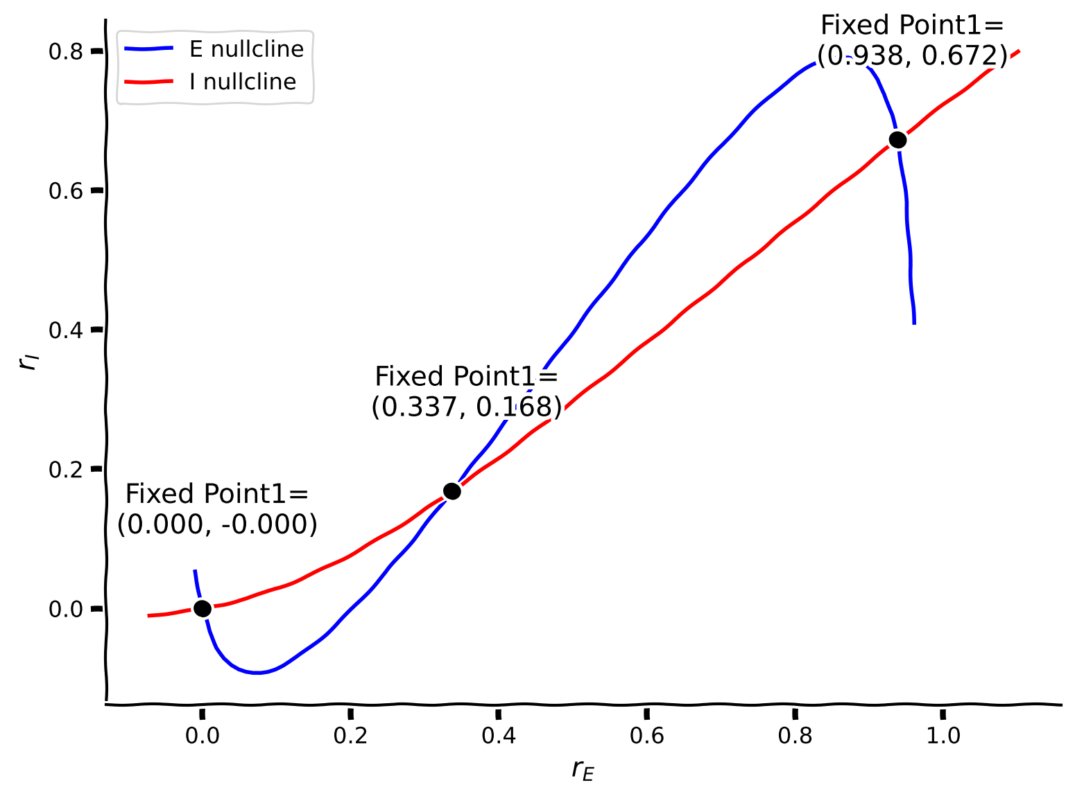
セクション1.1: E/Iシステムの固定点

2つのヌルクライン曲線の交点が、式 $(1)$ のWilson-Cowanモデルの固定点です。

次の演習では、与えられたパラメータセットに対してすべての固定点の座標を見つけます。

チュートリアル1で見たものと似た2つの関数を使います。これらは根探索アルゴリズムを用いて、興奮性および抑制性集団を持つシステムの固定点を見つけます。

# @markdown Execute to visualize nullclines

# Set parameters
pars = default_pars()
Exc_null_rE = np.linspace(-0.01, 0.96, 100)
Inh_null_rI = np.linspace(-.01, 0.8, 100)

# Compute nullclines
Exc_null_rI = get_E_nullcline(Exc_null_rE, **pars)
Inh_null_rE = get_I_nullcline(Inh_null_rI, **pars)

plot_nullclines(Exc_null_rE, Exc_null_rI, Inh_null_rE, Inh_null_rI)

# @markdown *Execute the cell to define `my_fp` and `check_fp`*

def my_fp(pars, rE_init, rI_init):
  """
  Use opt.root function to solve Equations (2)-(3) from initial values
  """

  tau_E, a_E, theta_E = pars['tau_E'], pars['a_E'], pars['theta_E']
  tau_I, a_I, theta_I = pars['tau_I'], pars['a_I'], pars['theta_I']
  wEE, wEI = pars['wEE'], pars['wEI']
  wIE, wII = pars['wIE'], pars['wII']
  I_ext_E, I_ext_I = pars['I_ext_E'], pars['I_ext_I']

  # define the right hand of wilson-cowan equations
  def my_WCr(x):

    rE, rI = x
    drEdt = (-rE + F(wEE * rE - wEI * rI + I_ext_E, a_E, theta_E)) / tau_E
    drIdt = (-rI + F(wIE * rE - wII * rI + I_ext_I, a_I, theta_I)) / tau_I
    y = np.array([drEdt, drIdt])

    return y

  x0 = np.array([rE_init, rI_init])
  x_fp = opt.root(my_WCr, x0).x

  return x_fp


def check_fp(pars, x_fp, mytol=1e-6):
  """
  Verify (drE/dt)^2 + (drI/dt)^2< mytol

  Args:
    pars    : Parameter dictionary
    fp      : value of fixed point
    mytol   : tolerance, default as 10^{-6}

  Returns :
    Whether it is a correct fixed point: True/False
  """

  drEdt, drIdt = EIderivs(x_fp[0], x_fp[1], **pars)

  return drEdt**2 + drIdt**2 < mytol

help(my_fp)

コーディング演習1.1: Wilson-Cowanモデルの固定点を見つける

上記のヌルクラインから、このシステムは使用したパラメータで3つの固定点を持つことがわかります。これらの座標を見つけるには、my_fp関数内のopt.root関数に適切な初期値を与える必要があります。アルゴリズムは初期値の近傍にある固定点しか見つけられないためです。

この演習では、初期値を変えてmy_fp関数を使い、それぞれの固定点を見つけます。ヌルクラインの交点付近の値を初期値として選ぶことができます。

pars = default_pars()

######################################################################
# TODO: Provide initial values to calculate the fixed points
# Check if x_fp's are the correct with the function check_fp(x_fp)
# Hint: vary different initial values to find the correct fixed points
raise NotImplementedError('student exercise: find fixed points')
######################################################################

my_plot_nullcline(pars)

# Find the first fixed point
x_fp_1 = my_fp(pars, ..., ...)
if check_fp(pars, x_fp_1):
  plot_fp(x_fp_1)

# Find the second fixed point
x_fp_2 = my_fp(pars, ..., ...)
if check_fp(pars, x_fp_2):
  plot_fp(x_fp_2)

# Find the third fixed point
x_fp_3 = my_fp(pars, ..., ...)
if check_fp(pars, x_fp_3):
  plot_fp(x_fp_3)

解答を見る$

出力例:

# @title Submit your feedback
content_review(f"{feedback_prefix}_Find_the_Fixed_points_of_WE_Exercise")

セクション1.2: 固定点の安定性とヤコビ行列の固有値

まず、システム $(1)$ を次のように書き換えます:

\begin{align}
$\frac{dr_E}{dt}$ &= $G_E(r_E,r_I)$ \
$\frac{dr_I}{dt}$ &= $G_I(r_E,r_I)$
\end{align}

ここで

\begin{align}
$G_E(r_E,r_I)$ &= $\frac{1}{\tau_E}$ [- $r_E$ + $F_E(w_{EE}r_E$ - $w_{EI}r_I$ + $I^{$ $\text{ext}}_E$ ;a, $\theta)$ ] \
$G_I(r_E,r_I)$ &= $\frac{1}{\tau_I}$ [- $r_I$ + $F_I(w_{IE}r_E$ - $w_{II}r_I$ + $I^{$ $\text{ext}}_I$ ;a, $\theta)$ ]
\end{align}

定義より、各固定点では $\displaystyle\frac{dr_E}{dt}=0$ および $\displaystyle\frac{dr_I}{dt}=0$ となります。したがって、初期状態が固定点に正確にある場合、時間が経っても状態は変化しません。

しかし、初期状態が固定点からわずかにずれた場合、2つの可能性があります。

軌道は固定点に引き戻される
軌道は固定点から発散する

これら2つの可能性が固定点の種類、すなわち安定か不安定かを決定します。前回のチュートリアルで学んだ1次元系と同様に、固定点 $(r_E^*, r_I^*)$ の安定性はシステムの動力学を線形化することで判定できます（方法はわかりますか？）。線形化により、ヤコビ行列と呼ばれる1次微分の行列が得られます:

J= \left[ {\begin{array} \displaystyle{\frac{\partial}{\partial r_E}}G_E(r_E^*, r_I^*) & \displaystyle{\frac{\partial}{\partial r_I}}G_E(r_E^*, r_I^*)\\[1mm] \displaystyle\frac{\partial}{\partial r_E} G_I(r_E^*, r_I^*) & \displaystyle\frac{\partial}{\partial r_I}G_I(r_E^*, r_I^*) \\ \end{array} } \right] \quad (7)

固定点で計算したヤコビ行列の固有値によって、その固定点が安定か不安定かが決まります。

ヤコビ行列を構成するために必要な微分を計算しましょう。連鎖律と積の法則を用いると、興奮性集団の微分は以下のようになります:

\begin{align}
$\frac{\partial}{\partial r_E} G_E(r_E^*, r_I^*)$ &= $\frac{1}{\tau_E}$ [-1 + $w_{EE}$ $F_E$ '( $w_{EE}r_E^*$ - $w_{EI}r_I^*$ + $I^{$ $\text{ext}}_E$ ; $\alpha_E, \theta_E)$ ] \[1mm]
$\frac{\partial}{\partial r_I} G_E(r_E^*, r_I^*)$ &= $\frac{1}{\tau_E}$ [- $w_{EI}$ $F_E$ '( $w_{EE}r_E^*$ - $w_{EI}r_I^*$ + $I^{$ $\text{ext}}_E$ ; $\alpha_E, \theta_E)$ ]
\end{align}

抑制性集団についても同様です。

コーディング演習1.2: Wilson-Cowanモデルのヤコビ行列を計算する

ここでは、Helper functionsで定義されたdF(x,a,theta)を使ってF-I曲線の微分を計算できます。

def get_eig_Jacobian(fp,
                     tau_E, a_E, theta_E, wEE, wEI, I_ext_E,
                     tau_I, a_I, theta_I, wIE, wII, I_ext_I, **other_pars):
  """Compute eigenvalues of the Wilson-Cowan Jacobian matrix at fixed point."""
  # Initialization
  rE, rI = fp
  J = np.zeros((2, 2))

  ###########################################################################
  # TODO for students: compute J and disable the error
  raise NotImplementedError("Student exercise: compute the Jacobian matrix")
  ###########################################################################
  # Compute the four elements of the Jacobian matrix
  J[0, 0] = ...
  J[0, 1] = ...
  J[1, 0] = ...
  J[1, 1] = ...

  # Compute and return the eigenvalues
  evals = np.linalg.eig(J)[0]
  return evals


# Compute eigenvalues of Jacobian
eig_1 = get_eig_Jacobian(x_fp_1, **pars)
eig_2 = get_eig_Jacobian(x_fp_2, **pars)
eig_3 = get_eig_Jacobian(x_fp_3, **pars)

print(eig_1, 'Stable point')
print(eig_2, 'Unstable point')
print(eig_3, 'Stable point')

解答を見る$

# @title Submit your feedback
content_review(f"{feedback_prefix}_Compute_the_Jacobian_Exercise")

明らかなように、安定な固定点は負の固有値に対応し、不安定な点は少なくとも1つの正の固有値を持ちます。

固有値の符号は興奮性と抑制性集団間の結合（相互作用）によって決まります。

以下では、 $w_{EE}$ がヌルクラインと動的システムの固有値に与える影響を調べます。

* 重要な変化は ピッチフォーク分岐 と呼ばれます。

セクション1.3: `wEE` がヌルクラインと固有値に与える影響

インタラクティブデモ1.3: パラメータ値によって位相平面のヌルクラインの位置が変化する

パラメータ $w_{EE}$ の値が異なるとヌルクラインはどのように動きますか？これは固定点やシステムの活動にどんな意味を持つでしょうか？

# @markdown Make sure you execute this cell to enable the widget!

@widgets.interact(
    wEE=widgets.FloatSlider(6., min=6., max=10., step=0.01)
)

def plot_nullcline_diffwEE(wEE):
  """
    plot nullclines for different values of wEE
  """

  pars = default_pars(wEE=wEE)

  # plot the E, I nullclines
  Exc_null_rE = np.linspace(-0.01, .96, 100)
  Exc_null_rI = get_E_nullcline(Exc_null_rE, **pars)

  Inh_null_rI = np.linspace(-.01, .8, 100)
  Inh_null_rE = get_I_nullcline(Inh_null_rI, **pars)

  plt.figure(figsize=(12, 5.5))
  plt.subplot(121)
  plt.plot(Exc_null_rE, Exc_null_rI, 'b', label='E nullcline')
  plt.plot(Inh_null_rE, Inh_null_rI, 'r', label='I nullcline')
  plt.xlabel(r'$r_E$')
  plt.ylabel(r'$r_I$')
  plt.legend(loc='best')

  plt.subplot(222)
  pars['rE_init'], pars['rI_init'] = 0.2, 0.2
  rE, rI = simulate_wc(**pars)
  plt.plot(pars['range_t'], rE, 'b', label='E population', clip_on=False)
  plt.plot(pars['range_t'], rI, 'r', label='I population', clip_on=False)
  plt.ylabel('Activity')
  plt.legend(loc='best')
  plt.ylim(-0.05, 1.05)
  plt.title('E/I activity\nfor different initial conditions',
            fontweight='bold')

  plt.subplot(224)
  pars['rE_init'], pars['rI_init'] = 0.4, 0.1
  rE, rI = simulate_wc(**pars)
  plt.plot(pars['range_t'], rE, 'b', label='E population', clip_on=False)
  plt.plot(pars['range_t'], rI, 'r', label='I population', clip_on=False)
  plt.xlabel('t (ms)')
  plt.ylabel('Activity')
  plt.legend(loc='best')
  plt.ylim(-0.05, 1.05)

  plt.tight_layout()
  plt.show()

解答を見る$

# @title Submit your feedback
content_review(f"{feedback_prefix}_Effect_of_wEE_Interactive_Demo_and_Discussion")

また、 $w_{EI}$ 、 $w_{IE}$ 、 $w_{II}$ 、 $\tau_{E}$ 、 $\tau_{I}$ 、および $I_{E}^{\text{ext}}$ の異なる値が固定点の安定性に与える影響も調べることができます。さらに、利得曲線 $F(\cdot)$ のパラメータの摂動も考慮できます。

セクション 1.4: リミットサイクル - 振動

相互作用項 ( $w_{EE}, w_{IE}, w_{EI}, w_{II}$ ) の値によっては、固有値が複素数になることがあります。少なくとも一組の固有値が複素数になると、振動が発生します。
振動の安定性は固有値の実部によって決まります（実部が正なら振動は増幅し、負なら振動は減衰します）。複素部の大きさは振動の周波数を決定します。

例えば、異なるパラメータセット $w_{EE}=6.4$ , $w_{EI}=4.8$ , $w_{IE}=6.$ , $w_{II}=1.2$ , および $I_{E}^{\text{ext}}=0.8$ を用いると、E と I の集団活動が振動し始めることが観察できます！以下のセルを実行して振動挙動を確認してください。

# @markdown Make sure you execute this cell to see the oscillations!

pars = default_pars(T=100.)
pars['wEE'], pars['wEI'] = 6.4, 4.8
pars['wIE'], pars['wII'] = 6.0, 1.2
pars['I_ext_E'] = 0.8
pars['rE_init'], pars['rI_init'] = 0.25, 0.25

rE, rI = simulate_wc(**pars)
plt.figure(figsize=(8, 5.5))
plt.plot(pars['range_t'], rE, 'b', label=r'$r_E$')
plt.plot(pars['range_t'], rI, 'r', label=r'$r_I$')
plt.xlabel('t (ms)')
plt.ylabel('Activity')
plt.legend(loc='best')
plt.show()

位相平面を用いて集団の振動を理解することもできます。異なる初期状態からの軌道を複数プロットすると、これらの軌道が固定点に収束するのではなく円を描いて動くことがわかります。この円は「リミットサイクル」と呼ばれ、特定の条件下での $E$ と $I$ 集団の周期的振動を示しています。

先に定義した関数を使って位相平面をプロットしてみましょう。

# @markdown Execute to visualize phase plane

pars = default_pars(T=100.)
pars['wEE'], pars['wEI'] = 6.4, 4.8
pars['wIE'], pars['wII'] = 6.0, 1.2
pars['I_ext_E'] = 0.8


plt.figure(figsize=(7, 5.5))
my_plot_nullcline(pars)

# Find the correct fixed point
x_fp_1 = my_fp(pars, 0.8, 0.8)
if check_fp(pars, x_fp_1):
  plot_fp(x_fp_1, position=(0, 0), rotation=40)

my_plot_trajectories(pars, 0.2, 3,
                      'Sample trajectories \nwith different initial values')

my_plot_vector(pars)

plt.legend(loc=[1.01, 0.7])
plt.xlim(-0.05, 1.01)
plt.ylim(-0.05, 0.65)
plt.show()

インタラクティブデモ 1.4: リミットサイクルと振動

上記の例から、モデルパラメータの変化はヌルクラインの形状を変え、それに応じて $E$ と $I$ 集団の挙動が定常固定点から振動へと変化します。しかし、ヌルクラインの形状だけではネットワークの挙動を完全に決定できません。ベクトル場も重要です。これを示すために、ここでは時間定数の影響を調べます。抑制性の時間定数 $\tau_I$ を変えると、ヌルクラインは変わりませんが、ネットワークの振る舞いは定常状態から異なる周波数の振動へと大きく変化します。

このようなシステム挙動の劇的な変化は分岐と呼ばれます。

以下のコードを実行して確認してください。

# @markdown Make sure you execute this cell to enable the widget!

@widgets.interact(
    tau_i=widgets.FloatSlider(1.5, min=0.2, max=3., step=.1)
)


def time_constant_effect(tau_i=0.5):

  pars = default_pars(T=100.)
  pars['wEE'], pars['wEI'] = 6.4, 4.8
  pars['wIE'], pars['wII'] = 6.0, 1.2
  pars['I_ext_E'] = 0.8

  pars['tau_I'] = tau_i

  Exc_null_rE = np.linspace(0.0, .9, 100)
  Inh_null_rI = np.linspace(0.0, .6, 100)

  Exc_null_rI = get_E_nullcline(Exc_null_rE, **pars)
  Inh_null_rE = get_I_nullcline(Inh_null_rI, **pars)

  plt.figure(figsize=(12.5, 5.5))

  plt.subplot(121)  # nullclines
  plt.plot(Exc_null_rE, Exc_null_rI, 'b', label='E nullcline', zorder=2)
  plt.plot(Inh_null_rE, Inh_null_rI, 'r', label='I nullcline', zorder=2)
  plt.xlabel(r'$r_E$')
  plt.ylabel(r'$r_I$')

  # fixed point
  x_fp_1 = my_fp(pars, 0.5, 0.5)
  plt.plot(x_fp_1[0], x_fp_1[1], 'ko', zorder=2)

  eig_1 = get_eig_Jacobian(x_fp_1, **pars)

  # trajectories
  for ie in range(5):
    for ii in range(5):
      pars['rE_init'], pars['rI_init'] = 0.1 * ie, 0.1 * ii
      rE_tj, rI_tj = simulate_wc(**pars)
      plt.plot(rE_tj, rI_tj, 'k', alpha=0.3, zorder=1)

  # vector field
  EI_grid_E = np.linspace(0., 1.0, 20)
  EI_grid_I = np.linspace(0., 0.6, 20)
  rE, rI = np.meshgrid(EI_grid_E, EI_grid_I)
  drEdt, drIdt = EIderivs(rE, rI, **pars)
  n_skip = 2
  plt.quiver(rE[::n_skip, ::n_skip], rI[::n_skip, ::n_skip],
              drEdt[::n_skip, ::n_skip], drIdt[::n_skip, ::n_skip],
              angles='xy', scale_units='xy', scale=10, facecolor='c')
  plt.title(r'$\tau_I=$'+'%.1f ms' % tau_i)

  plt.subplot(122)  # sample E/I trajectories
  pars['rE_init'], pars['rI_init'] = 0.25, 0.25
  rE, rI = simulate_wc(**pars)
  plt.plot(pars['range_t'], rE, 'b', label=r'$r_E$')
  plt.plot(pars['range_t'], rI, 'r', label=r'$r_I$')
  plt.xlabel('t (ms)')
  plt.ylabel('Activity')
  plt.title(r'$\tau_I=$'+'%.1f ms' % tau_i)
  plt.legend(loc='best')
  plt.tight_layout()
  plt.show()

$\tau_E$ と $\tau_I$ は二集団ネットワークのヤコビ行列（式7）に現れます。ここでは $\tau_I$ を増やすことで、安定な固定点に対応する固有値が複素数になっているようです。

直感的には、 $\tau_I$ が小さいと抑制性活動は興奮性活動より速く変化します。抑制がある値を超えると、高い抑制が興奮性集団を抑制しますが、それは逆に抑制性集団への入力（興奮性からの結合）が減ることを意味します。したがって抑制は急速に減少します。しかしこれは興奮が回復することを意味し・・・以下同様に繰り返されます。

# @title Submit your feedback
content_review(f"{feedback_prefix}_Limit_cycle_and_oscillations_Interactive_Demo")

セクション 2: 抑制安定化ネットワーク (ISN)

セクション 2.1: 抑制安定化ネットワーク

前述のように、固定点周りの線形近似は次のように得られます。

\frac{d}{dr} \vec{R} = \left[ {\begin{array} \displaystyle{\frac{\partial G_E}{\partial r_E}} & \displaystyle{\frac{\partial G_E}{\partial r_I}} \\ \displaystyle\frac{\partial G_I}{\partial r_E} & \displaystyle\frac{\partial G_I}{\partial r_I} \\ \end{array} } \right] \vec{R},

ここで $\vec{R} = [r_E, r_I]^{\rm T}$ は E/I 活動のベクトルです。

興奮性サブポピュレーションに注目すると、次のようになります。

\frac{dr_E}{dt} = \frac{\partial G_E}{\partial r_E}\cdot r_E + \frac{\partial G_E}{\partial r_I} \cdot r_I

固定点 $(r_E^*, r_I^*)$ 周りでの偏微分は次の通りです。

\begin{align}
$\frac{\partial}{\partial r_E}G_E(r_E^*, r_I^*)$ &= $\frac{1}{\tau_E}$ [-1 + $w_{EE}$ F'{ $E}(w_{EE}r_E^*$ - $w_{EI}r_I^*$ + $I^{$ $\text{ext}}_E$ ; $\alpha_E, \theta_E)$ ] & $\qquad (8)$ \
$\frac{\partial}{\partial r_I}G_E(r_E^*, r_I^*)$ &= $\frac{1}{\tau_E}$ [- $w_{EI}$ F'{ $E}(w_{EE}r_E^*$ - $w_{EI}r_I^*$ + $I^{$ $\text{ext}}_E$ ; $\alpha_E, \theta_E)$ ] & $\qquad (9)$ \
$\frac{\partial}{\partial r_E}G_I(r_E^*, r_I^*)$ &= $\frac{1}{\tau_I}$ [ $w_{IE}$ F'{ $I}(w_{IE}r_E^*$ - $w_{II}r_I^*$ + $I^{$ $\text{ext}}_I$ ; $\alpha_I, \theta_I)$ ] & $\qquad (10)$ \
$\frac{\partial}{\partial r_I}G_I(r_E^*, r_I^*)$ &= $\frac{1}{\tau_I}$ [-1- $w_{II}$ F'{ $I}(w_{IE}r_E^*$ - $w_{II}r_I^*$ + $I^{$ $\text{ext}}_I$ ; $\alpha_I, \theta_I)$ ] &$\qquad (11)
\end{align}

式(8)から、 $\displaystyle{\frac{\partial G_E}{\partial r_I}}$ は $\displaystyle{\frac{dF}{dx}}$ が常に正なので負であることがわかります。これは抑制性活動 ( $I$ ) からの再帰的抑制が興奮性 ( $E$ ) 活動を減少させるためです。しかし、前述のように $\displaystyle{\frac{\partial G_E}{\partial r_E}}$ は「リーク」効果に関連する負の項と再帰的興奮に関連する正の項を持ちます。したがって、2つの異なる状態が生じます。

$\displaystyle{\frac{\partial}{\partial r_E}G_E(r_E^*, r_I^*)}<0$ 、非抑制安定化ネットワーク (non-ISN) 状態
$\displaystyle{\frac{\partial}{\partial r_E}G_E(r_E^*, r_I^*)}>0$ 、抑制安定化ネットワーク (ISN) 状態

コーディング演習 2.1: $\displaystyle{\frac{\partial G_E}{\partial r_E}}$ を計算する

デフォルトパラメータとリミットサイクルの場合のパラメータで、 $\displaystyle{\frac{\partial G_E}{\partial r_E}}$ を計算する関数を実装してください。

def get_dGdE(fp, tau_E, a_E, theta_E, wEE, wEI, I_ext_E, **other_pars):
  """
  Compute dGdE

  Args:
    fp   : fixed point (E, I), array
    Other arguments are parameters of the Wilson-Cowan model

  Returns:
    J    : the 2x2 Jacobian matrix
  """
  rE, rI = fp

  ##########################################################################
  # TODO for students: compute dGdrE and disable the error
  raise NotImplementedError("Student exercise: compute the dG/dE, Eq. (13)")
  ##########################################################################
  # Calculate the J[0,0]
  dGdrE = ...

  return dGdrE


# Get fixed points
pars = default_pars()
x_fp_1 = my_fp(pars, 0.1, 0.1)
x_fp_2 = my_fp(pars, 0.3, 0.3)
x_fp_3 = my_fp(pars, 0.8, 0.6)

# Compute dGdE
dGdrE1 = get_dGdE(x_fp_1, **pars)
dGdrE2 = get_dGdE(x_fp_2, **pars)
dGdrE3 = get_dGdE(x_fp_3, **pars)

print(f'For the default case:')
print(f'dG/drE(fp1) = {dGdrE1:.3f}')
print(f'dG/drE(fp2) = {dGdrE2:.3f}')
print(f'dG/drE(fp3) = {dGdrE3:.3f}')

print('\n')

pars = default_pars(wEE=6.4, wEI=4.8, wIE=6.0, wII=1.2, I_ext_E=0.8)
x_fp_lc = my_fp(pars, 0.8, 0.8)

dGdrE_lc = get_dGdE(x_fp_lc, **pars)

print('For the limit cycle case:')
print(f'dG/drE(fp_lc) = {dGdrE_lc:.3f}')

実行例

デフォルトの場合:
dG/drE(fp1) = -0.650
dG/drE(fp2) = 1.519
dG/drE(fp3) = -0.706


リミットサイクルの場合:
dG/drE(fp_lc) = 0.837

解答を見る$

# @title Submit your feedback
content_review(f"{feedback_prefix}_Compute_dGdrE_Exercise")

セクション 2.2: ISNのヌルクライン解析

Eのヌルクラインは以下のように表されることを思い出してください。

r_E = F_E(w_{EE}r_E -w_{EI}r_I + I^{\text{ext}}_E;a_E,\theta_E).

つまり、発火率 $r_E$ は $r_I$ の関数となり得ます。 $r_E$ を $r_I$ で微分すると、以下が得られます。

\begin{align}
& $\frac{dr_E}{dr_I} = F_E' \cdot (w_{EE}\frac{dr_E}{dr_I} -w_{EI}) \iff$ \
&(1- $F_E$ ' $w_{EE})$ $\frac{dr_E}{dr_I} = -F_E' w_{EI} \iff$ \
& $\frac{dr_E}{dr_I} = \frac{F_E' w_{EI}}{F_E'w_{EE}-1}$ .
\end{align}

つまり、位相平面の rI-rE 平面上で、Eのヌルクラインに沿った傾きは次のように得られます。

\frac{dr_I}{dr_E} = \frac{F_E'w_{EE}-1}{F_E' w_{EI}} \qquad (12)

同様に、Iのヌルクラインに沿った傾きは次のように得られます。

\frac{dr_I}{dr_E} = \frac{F_I'w_{IE}}{F_I' w_{II}+1} \qquad (13)

ここで、式 (13) における $\Big{(} \displaystyle{\frac{dr_I}{dr_E}} \Big{)}_{\rm I-nullcline}$ は正であることがわかります。

しかし、式 (12) における $\Big{(} \displaystyle{\frac{dr_I}{dr_E}} \Big{)}_{\rm E-nullcline}$ の符号は $(F_E'w_{EE}-1)$ の符号に依存します。なお、 $(F_E'w_{EE}-1)$ は上記の式 (8) と同じものです。したがって、以下の結果が得られます。

$\Big{(} \displaystyle{\frac{dr_I}{dr_E}} \Big{)}_{\rm E-nullcline}<0$ の場合、非抑制安定化ネットワーク（non-ISN）領域
$\Big{(} \displaystyle{\frac{dr_I}{dr_E}} \Big{)}_{\rm E-nullcline}>0$ の場合、抑制安定化ネットワーク（ISN）領域

さらに、以下の2つの結論を指摘することが重要です。

結論1: 固定点の安定性は、式 (12) と (13) の傾きの関係を決定します。前述の通り、ヤコビ行列（式 (7) の $J$ ）の固有値が2つとも実部負である場合、固定点は安定であり、これは $J$ の行列式が正、すなわち $\text{det}(J)>0$ であることを意味します。

ヤコビ行列の定義と式 (8)-(11) から、次のように得られます。

J = \left[ {\begin{array} \displaystyle{\frac{1}{\tau_E}(w_{EE}F_E'-1)} & \displaystyle{-\frac{1}{\tau_E}w_{EI}F_E'}\\[1mm] \displaystyle {\frac{1}{\tau_I}w_{IE}F_I'}& \displaystyle {\frac{1}{\tau_I}(-w_{II}F_I'-1)} \\ \end{array} } \right]

ここで、次の行列を定義します。

T= \left[ { \begin{matrix} \displaystyle{\tau_E} & \displaystyle{0} \\ \displaystyle 0& \displaystyle \tau_I \end{matrix} } \right], F= \left[ { \begin{matrix} \displaystyle{F_E'} & \displaystyle{0} \\ \displaystyle 0& \displaystyle F_I' \end{matrix} } \right] \text{, および } W= \left[ { \begin{matrix} \displaystyle{w_{EE}} & \displaystyle{-w_{EI}} \\ \displaystyle w_{IE}& \displaystyle -w_{II} \end{matrix} } \right]

このとき、行列の記法を用いると、 $J=T^{-1}(F W - I)$ となり、ここで $I$ は単位行列、すなわち

\begin{bmatrix}
1 & 0 \
0 & 1
\end{bmatrix}

です。

したがって、 $\det{(J)}=\det{(T^{-1}(F W - I))}=(\det{(T^{-1})})(\det{(F W - I)})$ となります。

時間定数は定義上正なので、 $\det{(T^{-1})}>0$ であり、 $\det{(J)}$ の符号は $\det{(F W - I)}$ の符号と同じです。よって、

\det{(FW - I)} = (F_E' w_{EI})(F_I'w_{IE}) - (F_I' w_{II} + 1)(F_E'w_{EE} - 1) > 0.

これを式 (12) と (13) と組み合わせると、次の不等式が得られます。

\frac{\Big{(} \displaystyle{\frac{dr_I}{dr_E}} \Big{)}_{\rm I-nullcline}}{\Big{(} \displaystyle{\frac{dr_I}{dr_E}} \Big{)}_{\rm E-nullcline}} > 1.

したがって、安定な固定点においては、Iのヌルクラインの傾きはEのヌルクラインの傾きよりも急であることがわかります。

結論2: 抑制性集団への入力追加の効果。

抑制性集団に入力 $\delta I^{\rm ext}_I$ を加えると、Eのヌルクライン（式 (5)）は変わらず、Iのヌルクラインは純粋に左方向へシフトします。元のIのヌルクラインの式は

r_I = F_I(w_{IE}r_E-w_{II}r_I + I^{\text{ext}}_I ; \alpha_I, \theta_I)

であり、 $I^{\text{ext}}_I \rightarrow I^{\text{ext}}_I +\delta I^{\rm ext}_I$ とし、
$r_E\rightarrow r_E'=r_E-\frac{\delta I^{\rm ext}_I}{w_{IE}}$ と置くと、

r_I = F_I(w_{IE}r_E'-w_{II}r_I + I^{\text{ext}}_I +\delta I^{\rm ext}_I; \alpha_I, \theta_I)

となります。

これらをまとめると、以下の位相平面図が得られます。抑制性集団に入力を加えた後、ISN では、 $r_I$ は最初に増加しますが、その後新しい固定点に向かって減衰し、この新しい固定点では元の固定点と比べて $r_I$ と $r_E$ の両方が減少します。一方、非ISN に $\delta I^{\rm ext}_I$ を加えると、 $r_I$ は増加し、 $r_E$ は減少します。

インタラクティブデモ 2.2: 例の ISN と非ISN のヌルクライン

このインタラクティブウィジェットでは、システムが平衡状態にあるとき（パラメータは $w_{EE}=6.4$ , $w_{EI}=4.8$ , $w_{IE}=6.$ , $w_{II}=1.2$ , $I_{E}^{\text{ext}}=0.8$ , $\tau_I = 0.8$ , および $I^{\text{ext}}_I=0$ ）に、抑制性集団に興奮性ドライブ（ $I^{\text{ext}}_I>0$ ）または抑制性ドライブ（ $I^{\text{ext}}_I<0$ ）を注入します。抑制性集団への興奮性ドライブと抑制性ドライブで、 $I$ 集団の発火率はどのように変化するでしょうか？

# @title

# @markdown Make sure you execute this cell to enable the widget!

pars = default_pars(T=50., dt=0.1)
pars['wEE'], pars['wEI'] = 6.4, 4.8
pars['wIE'], pars['wII'] = 6.0, 1.2
pars['I_ext_E'] = 0.8
pars['tau_I'] = 0.8

@widgets.interact(
    dI=widgets.FloatSlider(0., min=-0.2, max=0.2, step=.05)
)


def ISN_I_perturb(dI=0.1):
  Lt = len(pars['range_t'])
  pars['I_ext_I'] = np.zeros(Lt)
  pars['I_ext_I'][int(Lt / 2):] = dI

  pars['rE_init'], pars['rI_init'] = 0.6, 0.26
  rE, rI = simulate_wc(**pars)

  plt.figure(figsize=(8, 1.5))

  plt.plot(pars['range_t'], pars['I_ext_I'], 'k')
  plt.xlabel('t (ms)')
  plt.ylabel(r'$I_I^{\mathrm{ext}}$')
  plt.ylim(pars['I_ext_I'].min() - 0.01, pars['I_ext_I'].max() + 0.01)
  plt.show()

  plt.figure(figsize=(8, 4.5))
  plt.plot(pars['range_t'], rE, 'b', label=r'$r_E$')
  plt.plot(pars['range_t'], rE[int(Lt / 2) - 1] * np.ones(Lt), 'b--')
  plt.plot(pars['range_t'], rI, 'r', label=r'$r_I$')
  plt.plot(pars['range_t'], rI[int(Lt / 2) - 1] * np.ones(Lt), 'r--')
  plt.ylim(0, 0.8)
  plt.xlabel('t (ms)')
  plt.ylabel('Activity')
  plt.legend(loc='best')
  plt.show()

解答を見る$

# @title Submit your feedback
content_review(f"{feedback_prefix}_Nullclines_of_ISN_and_nonISN_Interactive_Demo_and_Discussion")

セクション3: 不動点と作業記憶

実験で測定されたニューロンへの入力はしばしば非常にノイズが多いです（リンク$）。ここでは、ノイズのあるシナプス入力電流をオーンシュタイン・ウーレンベック（OU）過程としてモデル化しています。このOU過程は、以前のチュートリアルで何度か取り上げられています。

# @markdown Make sure you execute this cell to enable the function my_OU and plot the input current!


def my_OU(pars, sig, myseed=False):
  """
  Expects:
  pars       : parameter dictionary
  sig        : noise amplitute
  myseed     : random seed. int or boolean

  Returns:
  I          : Ornstein-Uhlenbeck input current
  """

  # Retrieve simulation parameters
  dt, range_t = pars['dt'], pars['range_t']
  Lt = range_t.size
  tau_ou = pars['tau_ou']  # [ms]

  # set random seed
  if myseed:
      np.random.seed(seed=myseed)
  else:
      np.random.seed()

  # Initialize
  noise = np.random.randn(Lt)
  I_ou = np.zeros(Lt)
  I_ou[0] = noise[0] * sig

  # generate OU
  for it in range(Lt-1):
      I_ou[it+1] = (I_ou[it]
                    + dt / tau_ou * (0. - I_ou[it])
                    + np.sqrt(2 * dt / tau_ou) * sig * noise[it + 1])
  return I_ou


pars = default_pars(T=50)
pars['tau_ou'] = 1.  # [ms]
sig_ou = 0.1
I_ou = my_OU(pars, sig=sig_ou, myseed=2020)
plt.figure(figsize=(8, 5.5))
plt.plot(pars['range_t'], I_ou, 'b')
plt.xlabel('Time (ms)')
plt.ylabel(r'$I_{\mathrm{OU}}$')
plt.show()

デフォルトのパラメータでは、システムはノイズのある入力により安静状態の周りで変動します。

# @markdown Execute this cell to plot activity with noisy input current
pars = default_pars(T=100)
pars['tau_ou'] = 1.  # [ms]
sig_ou = 0.1
pars['I_ext_E'] = my_OU(pars, sig=sig_ou, myseed=20201)
pars['I_ext_I'] = my_OU(pars, sig=sig_ou, myseed=20202)

pars['rE_init'], pars['rI_init'] = 0.1, 0.1
rE, rI = simulate_wc(**pars)

plt.figure(figsize=(8, 5.5))
ax = plt.subplot(111)
ax.plot(pars['range_t'], rE, 'b', label='E population')
ax.plot(pars['range_t'], rI, 'r', label='I population')
ax.set_xlabel('t (ms)')
ax.set_ylabel('Activity')
ax.legend(loc='best')
plt.show()

インタラクティブデモ3：短いパルスによる持続的活動の誘発

次に、システムが平衡状態にあるときに、E集団に対して10msの短い正の電流を加えます。この振幅（以下のSE）が十分に大きい場合、一過性の入力を超えて持続的な活動が生じます。持続的活動の発火率はどのくらいで、臨界入力強度はいくつでしょうか？上記の位相平面解析からこの現象を理解してみてください。

# @markdown Make sure you execute this cell to enable the widget!
def my_inject(pars, t_start, t_lag=10.):
  """
  Expects:
  pars       : parameter dictionary
  t_start    : pulse starts [ms]
  t_lag      : pulse lasts  [ms]

  Returns:
  I          : extra pulse time
  """

  # Retrieve simulation parameters
  dt, range_t = pars['dt'], pars['range_t']
  Lt = range_t.size

  # Initialize
  I = np.zeros(Lt)

  # pulse timing
  N_start = int(t_start / dt)
  N_lag = int(t_lag / dt)
  I[N_start:N_start + N_lag] = 1.

  return I


pars = default_pars(T=100)
pars['tau_ou'] = 1.  # [ms]
sig_ou = 0.1
pars['I_ext_I'] = my_OU(pars, sig=sig_ou, myseed=2021)
pars['rE_init'], pars['rI_init'] = 0.1, 0.1


# pulse
I_pulse = my_inject(pars, t_start=20., t_lag=10.)
L_pulse = sum(I_pulse > 0.)

@widgets.interact(
    SE=widgets.FloatSlider(0., min=0., max=1., step=.05)
)


def WC_with_pulse(SE=0.):
  pars['I_ext_E'] = my_OU(pars, sig=sig_ou, myseed=2022)
  pars['I_ext_E'] += SE * I_pulse

  rE, rI = simulate_wc(**pars)

  plt.figure(figsize=(8, 5.5))
  ax = plt.subplot(111)
  ax.plot(pars['range_t'], rE, 'b', label='E population')
  ax.plot(pars['range_t'], rI, 'r', label='I population')

  ax.plot(pars['range_t'][I_pulse > 0.], 1.0*np.ones(L_pulse), 'r', lw=3.)
  ax.text(25, 1.05, 'stimulus on', horizontalalignment='center',
          verticalalignment='bottom')
  ax.set_ylim(-0.03, 1.2)
  ax.set_xlabel('t (ms)')
  ax.set_ylabel('Activity')
  ax.legend(loc='best')
  plt.show()

解答を見る$

# @title Submit your feedback
content_review(f"{feedback_prefix}_Persistent_activity_Interactive_Demo_and_Discussion")

抑制性集団に2回目の短い電流を加えたときに何が起こるかを探ってみましょう。

ボーナスチュートリアル: Wilson-Cowanモデルの拡張

チュートリアルの目的

セットアップ

セクション1: Wilson-Cowanモデルの固定点、安定性解析、リミットサイクル

セクション1.1: E/Iシステムの固定点

コーディング演習1.1: Wilson-Cowanモデルの固定点を見つける

セクション1.2: 固定点の安定性とヤコビ行列の固有値

コーディング演習1.2: Wilson-Cowanモデルのヤコビ行列を計算する

セクション1.3: wEE がヌルクラインと固有値に与える影響

インタラクティブデモ1.3: パラメータ値によって位相平面のヌルクラインの位置が変化する

セクション 1.4: リミットサイクル - 振動

インタラクティブデモ 1.4: リミットサイクルと振動

セクション 2: 抑制安定化ネットワーク (ISN)

セクション 2.1: 抑制安定化ネットワーク

コーディング演習 2.1: ∂GE∂rE\displaystyle{\frac{\partial G_E}{\partial r_E}}∂rE​∂GE​​ を計算する

セクション 2.2: ISNのヌルクライン解析

インタラクティブデモ 2.2: 例の ISN と 非ISN のヌルクライン

セクション3: 不動点と作業記憶

インタラクティブデモ3：短いパルスによる持続的活動の誘発

セクション1.3: `wEE` がヌルクラインと固有値に与える影響

コーディング演習 2.1: $\displaystyle{\frac{\partial G_E}{\partial r_E}}$ を計算する

インタラクティブデモ 2.2: 例の ISN と非ISN のヌルクライン