脳内で記録される豊かなダイナミクスの多くは、興奮性および抑制性ニューロンサブタイプの相互作用によって生成されます。ここでは、前回のチュートリアルと同様に、EおよびIの2つの結合した集団をモデル化します（Wilson-Cowanモデル）。興奮性または抑制性集団のダイナミクスを表す2つの結合微分方程式を記述できます：

\begin{align}
$\tau_E \frac{dr_E}{dt}$ &= -$r_E$ + $F_E(w_{EE}r_E$ -$w_{EI}r_I$ + I^{\text{ext}}_E;a_E,$\theta_E)$\
$\tau_I \frac{dr_I}{dt}$ &= -$r_I$ + $F_I(w_{IE}r_E$ -$w_{II}r_I$ + I^{\text{ext}}_I;a_I,\theta_I) \qquad (1) \end{align}

$r_E(t)$ は時刻 $t$ における興奮性集団の平均活性化（または発火率）、$r_I(t)$ は抑制性集団の活性化（または発火率）を表します。パラメータ $\tau_E$ と $\tau_I$ はそれぞれの集団のダイナミクスの時間スケールを制御します。結合強度は $w_{EE}$（E→E）、$w_{EI}$（I→E）、$w_{IE}$（E→I）、$w_{II}$（I→I）で与えられます。$w_{EI}$ と $w_{IE}$ はそれぞれ抑制性から興奮性集団への結合、及びその逆を表します。伝達関数（またはF-I曲線）$F_E(x;a_E,\theta_E)$ と $F_I(x;a_I,\theta_I)$ は興奮性および抑制性集団で異なる場合があります。

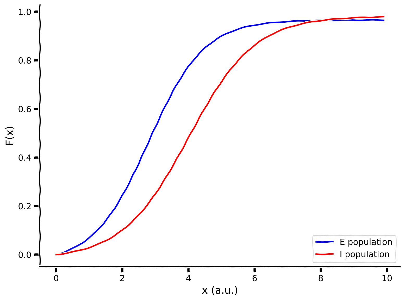
コーディング演習 1.1: EおよびI集団のF-I曲線をプロットしよう

まずはヘルパー関数 F を用いて、デフォルトパラメータでEおよびI集団のF-I曲線をプロットしましょう。

help(F)

pars = default_pars()
x = np.arange(0, 10, .1)

print(pars['a_E'], pars['theta_E'])
print(pars['a_I'], pars['theta_I'])

###################################################################
# TODO for students: compute and plot the F-I curve here          #
# Note: aE, thetaE, aI and theta_I are in the dictionary 'pairs'   #
raise NotImplementedError('student exercise: compute F-I curves of excitatory and inhibitory populations')
###################################################################

# Compute the F-I curve of the excitatory population
FI_exc = ...

# Compute the F-I curve of the inhibitory population
FI_inh = ...

# Visualize
plot_FI_EI(x, FI_exc, FI_inh)

解答を見る$

出力例:

# @title Submit your feedback
content_review(f"{feedback_prefix}_Plot_FI_Exercise")

セクション 1.2: Wilson-Cowanモデルのシミュレーションスキーム

チュートリアル開始からここまでの推定時間: 20分

再び、オイラー法を用いて方程式を数値積分できます。EおよびI集団のダイナミクスはステップ幅 $\Delta t$ の時間グリッド上でシミュレート可能です。興奮性および抑制性集団の活動の更新は以下のように書けます：

\begin{align}
r_E[k+1] &= r_E[k] + $\Delta r_E$[k]\
r_I[k+1] &= r_I[k] + $\Delta r_I$[k]
\end{align}

増分は

\begin{align}
$\Delta r_E$[k] &= $\frac{\Delta t}{\tau_E}$[-r_E[k] + $F_E(w_{EE}r_E[k]$ -$w_{EI}r_I[k]$ + I^{\text{ext}}_E[k];a_E,$\theta_E)$]\
$\Delta r_I$[k] &= $\frac{\Delta t}{\tau_I}$[-r_I[k] + $F_I(w_{IE}r_E[k]$ -$w_{II}r_I[k]$ + I^{\text{ext}}_I[k];a_I,$\theta_I)$]
\end{align}

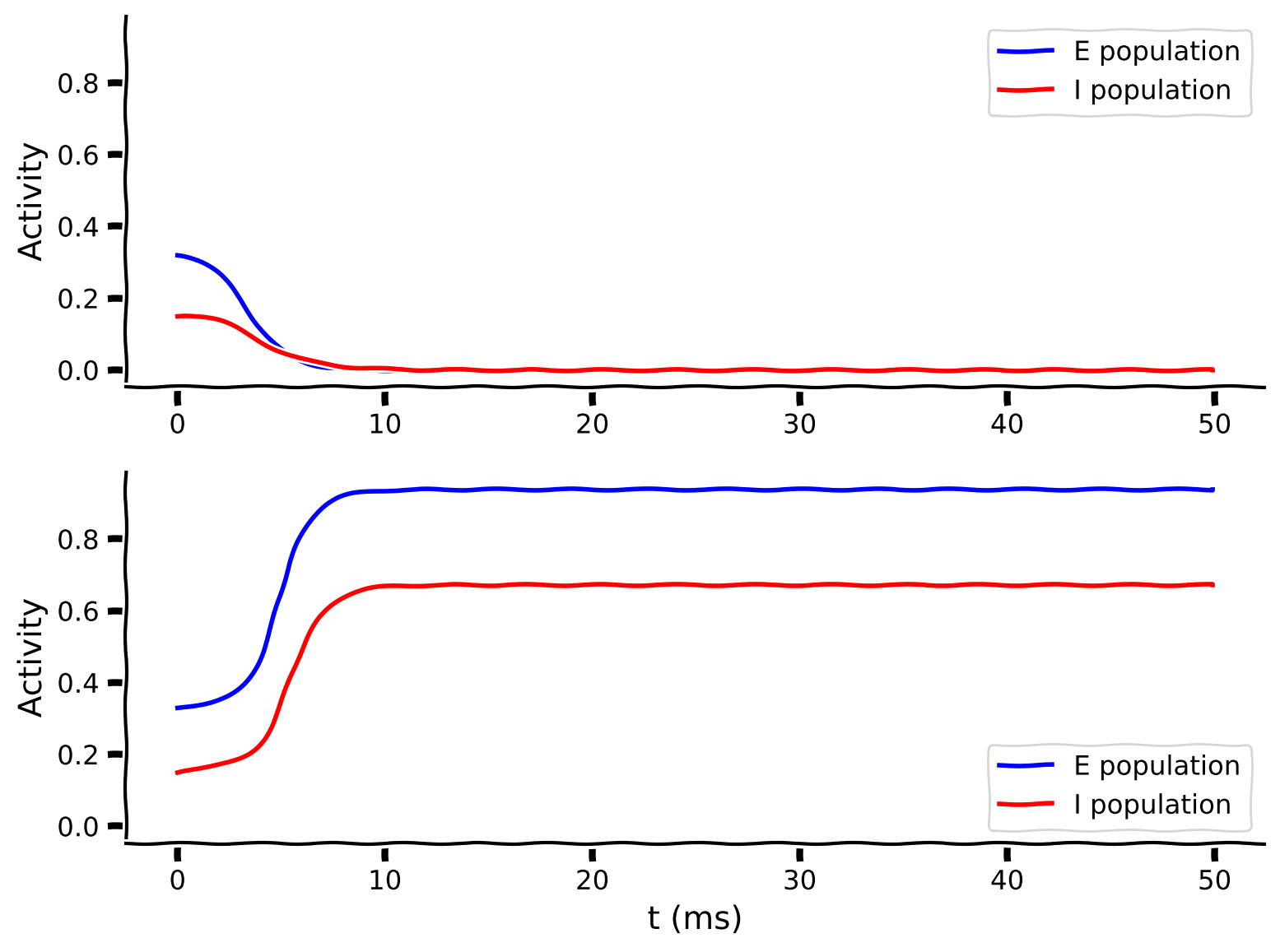
コーディング演習 1.2: Wilson-Cowan方程式を数値積分しよう

この数値シミュレーションを実装し、似た初期値での2つのシミュレーションを可視化します。

def simulate_wc(tau_E, a_E, theta_E, tau_I, a_I, theta_I,
                wEE, wEI, wIE, wII, I_ext_E, I_ext_I,
                rE_init, rI_init, dt, range_t, **other_pars):
  """
  Simulate the Wilson-Cowan equations

  Args:
    Parameters of the Wilson-Cowan model

  Returns:
    rE, rI (arrays) : Activity of excitatory and inhibitory populations
  """
  # Initialize activity arrays
  Lt = range_t.size
  rE = np.append(rE_init, np.zeros(Lt - 1))
  rI = np.append(rI_init, np.zeros(Lt - 1))
  I_ext_E = I_ext_E * np.ones(Lt)
  I_ext_I = I_ext_I * np.ones(Lt)

  # Simulate the Wilson-Cowan equations
  for k in range(Lt - 1):

    ########################################################################
    # TODO for students: compute drE and drI and remove the error
    raise NotImplementedError("Student exercise: compute the change in E/I")
    ########################################################################

    # Calculate the derivative of the E population
    drE = ...

    # Calculate the derivative of the I population
    drI = ...

    # Update using Euler's method
    rE[k + 1] = rE[k] + drE
    rI[k + 1] = rI[k] + drI

  return rE, rI


pars = default_pars()

# Simulate first trajectory
rE1, rI1 = simulate_wc(**default_pars(rE_init=.32, rI_init=.15))

# Simulate second trajectory
rE2, rI2 = simulate_wc(**default_pars(rE_init=.33, rI_init=.15))

# Visualize
my_test_plot(pars['range_t'], rE1, rI1, rE2, rI2)

解答を見る$

出力例:

# @title Submit your feedback
content_review(f"{feedback_prefix}_Numerical_Integration_of_WE_model_Exercise")

上の2つのプロットは、異なる初期条件での興奮性（$r_E$, 青）および抑制性（$r_I$, 赤）活動の時間発展を示しています。

インタラクティブデモ 1.2: 異なる初期値での集団軌道

このインタラクティブデモではWilson-Cowanモデルをシミュレートし、各集団の軌道をプロットします。興奮性集団の初期活動を変化させます。

異なる初期条件でEおよびI集団の軌道はどう変わるでしょうか？

# @markdown Make sure you execute this cell to enable the widget!
@widgets.interact(
    rE_init=widgets.FloatSlider(0.32, min=0.30, max=0.35, step=.01)
)


def plot_EI_diffinitial(rE_init=0.0):

  pars = default_pars(rE_init=rE_init, rI_init=.15)
  rE, rI = simulate_wc(**pars)

  plt.figure()
  plt.plot(pars['range_t'], rE, 'b', label='E population')
  plt.plot(pars['range_t'], rI, 'r', label='I population')
  plt.xlabel('t (ms)')
  plt.ylabel('Activity')
  plt.legend(loc='best')
  plt.show()

解答を見る$

# @title Submit your feedback
content_review(f"{feedback_prefix}_Population_trajectories_with_different_initial_values_Interactive_Demo_and_Discussion")

考えてみよう! 1.2

異なる初期状態を選ぶと神経応答の定常状態が異なることが明らかです。なぜでしょうか？

次のセクションで議論しますが、まずは考えてみてください。

セクション 2: 位相平面解析

チュートリアル開始からここまでの推定時間: 45分

前回のチュートリアルで1次元システムのダイナミクスを調べるためにグラフィカル手法を使ったように、ここではWilson-Cowanモデルのような2次元システムのダイナミクスを調べるための位相平面解析というグラフィカル手法を学びます。これは前提条件の微積分の日や線形システムの日で既に見たことがあります。

これまで、2つの集団の活動を時間の関数としてプロットしてきました。すなわち、Activity-t 平面、つまり $(t, r_E(t))$ 平面または $(t, r_I(t))$ 平面です。代わりに、任意の時刻 $t$ における2つの活動 $r_E(t)$ と $r_I(t)$ を互いに対してプロットできます。この rI-rE 平面 $(r_I(t), r_E(t))$ を位相平面と呼びます。位相平面の各点は、$r_E$ と $r_I$ の両方が時間とともにどのように変化するかを示します。

# @title Video 2: Nullclines and Vector Fields
from ipywidgets import widgets
from IPython.display import YouTubeVideo
from IPython.display import IFrame
from IPython.display import display


class PlayVideo(IFrame):
  def __init__(self, id, source, page=1, width=400, height=300, **kwargs):
    self.id = id
    if source == 'Bilibili':
      src = f'https://player.bilibili.com/player.html?bvid={id}&page={page}'
    elif source == 'Osf':
      src = f'https://mfr.ca-1.osf.io/render?url=https://osf.io/download/{id}/?direct%26mode=render'
    super(PlayVideo, self).__init__(src, width, height, **kwargs)


def display_videos(video_ids, W=400, H=300, fs=1):
  tab_contents = []
  for i, video_id in enumerate(video_ids):
    out = widgets.Output()
    with out:
      if video_ids[i][0] == 'Youtube':
        video = YouTubeVideo(id=video_ids[i][1], width=W,
                             height=H, fs=fs, rel=0)
        print(f'Video available at https://youtube.com/watch?v={video.id}')
      else:
        video = PlayVideo(id=video_ids[i][1], source=video_ids[i][0], width=W,
                          height=H, fs=fs, autoplay=False)
        if video_ids[i][0] == 'Bilibili':
          print(f'Video available at https://www.bilibili.com/video/{video.id}')
        elif video_ids[i][0] == 'Osf':
          print(f'Video available at https://osf.io/{video.id}')
      display(video)
    tab_contents.append(out)
  return tab_contents


video_ids = [('Youtube', 'V2SBAK2Xf8Y'), ('Bilibili', 'BV15k4y1m7Kt')]
tab_contents = display_videos(video_ids, W=854, H=480)
tabs = widgets.Tab()
tabs.children = tab_contents
for i in range(len(tab_contents)):
  tabs.set_title(i, video_ids[i][0])
display(tabs)

# @title Submit your feedback
content_review(f"{feedback_prefix}_Nullclines_and_Vector_Fields_Video")

インタラクティブデモ 2: 活動-時間平面から**$r_I$ - $r_E$**位相平面へ

このデモでは、Activity-time と (rE, rI) 位相平面の両方でシステムのダイナミクスを可視化します。円は時刻 $t$ における活動を示し、線はシミュレーション全期間のシステムの進化を表します。

時間スライダーを動かして、上のプロットが下のプロットにどう対応しているか理解しましょう。下のプロットには時間の明示的な情報はありますか？どんな情報を与えてくれますか？

# @markdown Make sure you execute this cell to enable the widget!

pars = default_pars(T=10, rE_init=0.6, rI_init=0.8)
rE, rI = simulate_wc(**pars)

@widgets.interact(
    n_t=widgets.IntSlider(0, min=0, max=len(pars['range_t']) - 1, step=1)
)


def plot_activity_phase(n_t):
  plt.figure(figsize=(8, 5.5))
  plt.subplot(211)
  plt.plot(pars['range_t'], rE, 'b', label=r'$r_E$')
  plt.plot(pars['range_t'], rI, 'r', label=r'$r_I$')
  plt.plot(pars['range_t'][n_t], rE[n_t], 'bo')
  plt.plot(pars['range_t'][n_t], rI[n_t], 'ro')
  plt.axvline(pars['range_t'][n_t], 0, 1, color='k', ls='--')
  plt.xlabel('t (ms)', fontsize=14)
  plt.ylabel('Activity', fontsize=14)
  plt.legend(loc='best', fontsize=14)

  plt.subplot(212)
  plt.plot(rE, rI, 'k')
  plt.plot(rE[n_t], rI[n_t], 'ko')
  plt.xlabel(r'$r_E$', fontsize=18, color='b')
  plt.ylabel(r'$r_I$', fontsize=18, color='r')

  plt.tight_layout()
  plt.show()

解答を見る$

# @title Submit your feedback
content_review(f"{feedback_prefix}_Time_plane_to_Phase_plane_Interactive_Demo_and_Discussion")

セクション 2.1: Wilson-Cowan方程式のヌルクライン

チュートリアル開始からここまでの推定時間: 1時間3分

位相平面解析の重要な概念に「ヌルクライン」があります。これは、ある集団の活動が変化しない点の集合（ただし必ずしも他方の集団は含まない）として定義されます。

言い換えれば、式(1)の$E$および$I$のヌルクラインは、それぞれ $\displaystyle{\frac{dr_E}{dt}}=0$ および $\displaystyle\frac{dr_I}{dt}=0$ となる点の集合です。すなわち：

\begin{align}
-$r_E$ + $F_E(w_{EE}r_E$ -$w_{EI}r_I$ + I^{\text{ext}}_E;a_E,$\theta_E)$ &= 0 $\qquad (2)$\[1mm]
-$r_I$ + $F_I(w_{IE}r_E$ -$w_{II}r_I$ + I^{\text{ext}}_I;a_I,$\theta_I)$ &= 0 \qquad (3) \end{align}

コーディング演習 2.1: Wilson-Cowanモデルのヌルクラインを計算しよう

次の演習では、EおよびI集団のヌルクラインを計算しプロットします。

興奮性集団のヌルクライン（式2）に沿って、式2を変形して抑制性活動を計算できます：

\begin{align}
$r_I$ = \frac{1}{w_{EI}}\big{[}w_{EE}r_E - F_E^{-1}(r_E; a_E,\theta_E) + I^{\text{ext}}_E \big{]}. \qquad(4) \end{align}

ここで $F_E^{-1}(r_E; a_E,\theta_E)$ は興奮性伝達関数の逆関数（以下で定義）です。式4は $r_E$ ヌルクラインを定義します。

抑制性集団のヌルクライン（式3）に沿って、式3を変形して興奮性活動を計算できます：
\begin{align}
$r_E$ = \frac{1}{w_{IE}} \big{[} w_{II}r_I + F_I^{-1}(r_I;a_I,\theta_I) - I^{\text{ext}}_I \big{]} \qquad (5) \end{align}

ここで $F_I^{-1}(r_I; a_I,\theta_I)$ は抑制性伝達関数の逆関数（以下で定義）です。式5は $I$ ヌルクラインを定義します。

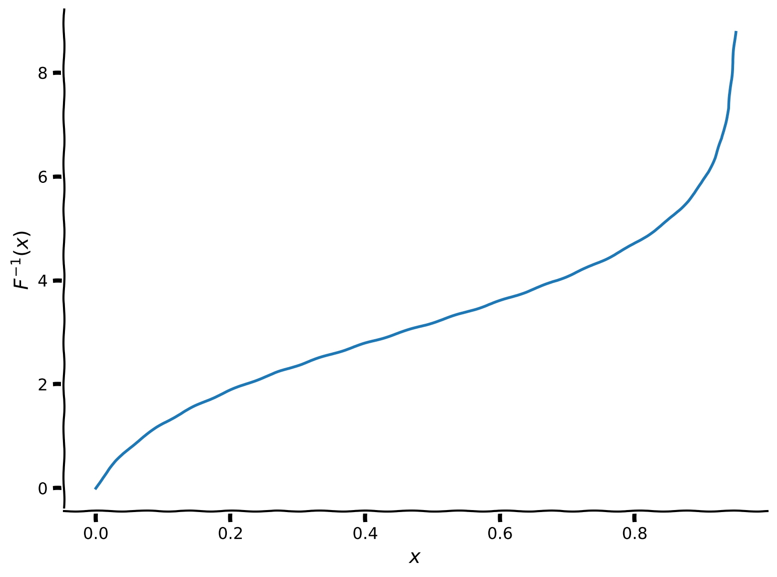
式4-5でヌルクラインを計算する際には、伝達関数の逆関数を計算する必要があります。

我々が用いているシグモイド型のf-I関数の逆関数は以下の通りです：

まずは逆伝達関数を実装しましょう：

def F_inv(x, a, theta):
  """
  Args:
    x         : the population input
    a         : the gain of the function
    theta     : the threshold of the function

  Returns:
    F_inverse : value of the inverse function
  """

  #########################################################################
  # TODO for students: compute F_inverse
  raise NotImplementedError("Student exercise: compute the inverse of F(x)")
  #########################################################################

  # Calculate Finverse (ln(x) can be calculated as np.log(x))
  F_inverse = ...

  return F_inverse


# Set parameters
pars = default_pars()
x = np.linspace(1e-6, 1, 100)

# Get inverse and visualize
plot_FI_inverse(x, a=1, theta=3)

解答を見る$

これで式4-5（以下に再掲）を用いてヌルクラインを計算できます：

\begin{align}
$r_I$ &= \frac{1}{w_{EI}}\big{[}w_{EE}r_E - F_E^{-1}(r_E; a_E,\theta_E) + I^{\text{ext}}_E \big{]} &$\qquad(4)$ \
$r_E$ &= \frac{1}{w_{IE}} \big{[} w_{II}r_I + F_I^{-1}(r_I;a_I,\theta_I) - I^{\text{ext}}_I \big{]} &\qquad (5) \end{align}

def get_E_nullcline(rE, a_E, theta_E, wEE, wEI, I_ext_E, **other_pars):
  """
  Solve for rI along the rE from drE/dt = 0.

  Args:
    rE    : response of excitatory population
    a_E, theta_E, wEE, wEI, I_ext_E : Wilson-Cowan excitatory parameters
    Other parameters are ignored

  Returns:
    rI    : values of inhibitory population along the nullcline on the rE
  """
  #########################################################################
  # TODO for students: compute rI for rE nullcline and disable the error
  raise NotImplementedError("Student exercise: compute the E nullcline")
  #########################################################################

  # calculate rI for E nullclines on rI
  rI = ...

  return rI


def get_I_nullcline(rI, a_I, theta_I, wIE, wII, I_ext_I, **other_pars):
  """
  Solve for E along the rI from dI/dt = 0.

  Args:
    rI    : response of inhibitory population
    a_I, theta_I, wIE, wII, I_ext_I : Wilson-Cowan inhibitory parameters
    Other parameters are ignored

  Returns:
    rE    : values of the excitatory population along the nullcline on the rI
  """
  #########################################################################
  # TODO for students: compute rI for rE nullcline and disable the error
  raise NotImplementedError("Student exercise: compute the I nullcline")
  #########################################################################

  # calculate rE for I nullclines on rI
  rE = ...

  return rE


# Set parameters
pars = default_pars()
Exc_null_rE = np.linspace(-0.01, 0.96, 100)
Inh_null_rI = np.linspace(-.01, 0.8, 100)

# Compute nullclines
Exc_null_rI = get_E_nullcline(Exc_null_rE, **pars)
Inh_null_rE = get_I_nullcline(Inh_null_rI, **pars)

# Visualize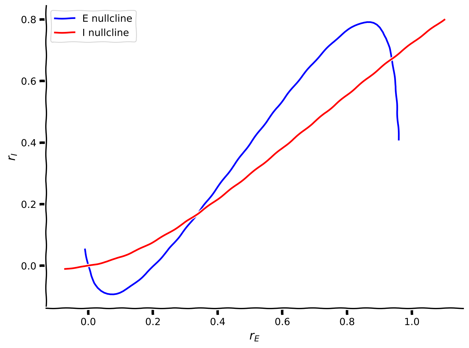
plot_nullclines(Exc_null_rE, Exc_null_rI, Inh_null_rE, Inh_null_rI)

解答を見る$

出力例:

# @title Submit your feedback
content_review(f"{feedback_prefix}_Compute_the_nullclines_WE_Exercise")

位相平面上の青線に沿っては $\displaystyle{\frac{dr_E(t)}{dt}} = 0$ であるため、この線はヌルクラインと呼ばれます。

つまり、青のヌルクラインは $r_E, r_I$ で張られた位相平面を2つの領域に分けます。ヌルクラインの片側では $\displaystyle{\frac{dr_E(t)}{dt}} > 0$、もう片側では $\displaystyle{\frac{dr_E(t)}{dt}} < 0$ となります。

同様に、赤線に沿っては $\displaystyle{\frac{dr_I(t)}{dt}} = 0$ であり、赤のヌルクラインは位相平面を2つの領域に分けます。片側では $\displaystyle{\frac{dr_I(t)}{dt}} > 0$、もう片側では $\displaystyle{\frac{dr_I(t)}{dt}} < 0$ となります。

セクション 2.2: ベクトル場

チュートリアル開始からここまでの推定時間: 1時間20分

位相平面とヌルクラインはWilson-Cowanモデルの挙動理解にどう役立つでしょうか？

関連ビデオ内容のテキスト要約はこちらをクリック

$E$および$I$集団の活動 $r_E(t)$ と $r_I(t)$ は時刻 $t$ における位相平面上の点 $(r_E(t),r_I(t))$ に対応します。したがって、システムの時間依存軌道は位相平面上の連続曲線として表され、その軌道の接ベクトルはベクトル \bigg{(}\displaystyle{\frac{dr_E(t)}{dt},\frac{dr_I(t)}{dt}}\bigg{)} で定義されます。このベクトルは活動がどの方向にどの速さで変化しているかを示します。実際、位相平面上の任意の点 $(E,I)$ で接ベクトル \bigg{(}\displaystyle{\frac{dr_E}{dt},\frac{dr_I}{dt}}\bigg{)} を計算でき、システムがその点を通過するときの挙動を示します。

位相平面上の接ベクトルのマップはベクトル場と呼ばれます。軌道の挙動は i) 初期条件 $(r_E(0),r_I(0))$ と ii) ベクトル場 \bigg{(}\displaystyle{\frac{dr_E(t)}{dt},\frac{dr_I(t)}{dt}}\bigg{)} によって決まります。

一般に、位相平面上の特定の点でのベクトル場の値は矢印で表されます。矢印の向きと大きさはそれぞれベクトルの方向とノルムを反映します。

コーディング演習 2.2: ベクトル場 \displaystyle{\Big{(}\frac{dr_E}{dt}, \frac{dr_I}{dt} \Big{)}} を計算・プロットしよう

以下の式に注意してください：

\begin{align}
$\frac{dr_E}{dt}$ &= [-$r_E$ + $F_E(w_{EE}r_E$ -$w_{EI}r_I$ + I^{\text{ext}}_E;a_E,$\theta_E)$]$\frac{1}{\tau_E}$\
$\frac{dr_I}{dt}$ &= [-$r_I$ + $F_I(w_{IE}r_E$ -$w_{II}r_I$ + I^{\text{ext}}_I;a_I,$\theta_I)$]\frac{1}{\tau_I} \end{align}

def EIderivs(rE, rI,
             tau_E, a_E, theta_E, wEE, wEI, I_ext_E,
             tau_I, a_I, theta_I, wIE, wII, I_ext_I,
             **other_pars):
  """Time derivatives for E/I variables (dE/dt, dI/dt)."""
  ######################################################################
  # TODO for students: compute drEdt and drIdt and disable the error
  raise NotImplementedError("Student exercise: compute the vector field")
  ######################################################################

  # Compute the derivative of rE
  drEdt = ...

  # Compute the derivative of rI
  drIdt = ...

  return drEdt, drIdt


# Create vector field using EIderivs
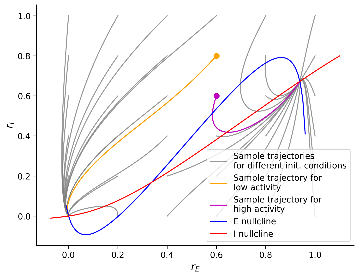
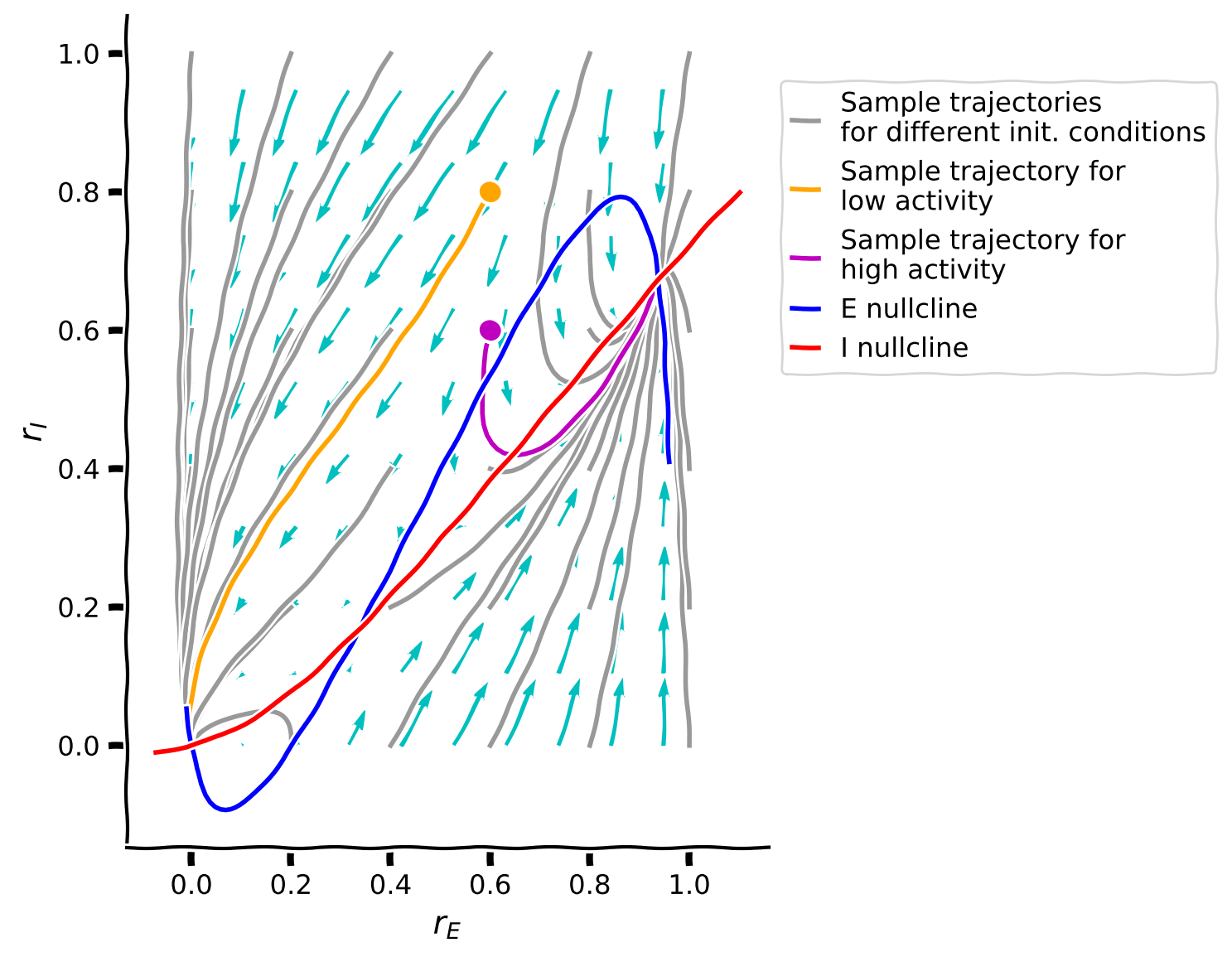
plot_complete_analysis(default_pars())

解答を見る$

出力例:

# @title Submit your feedback
content_review(f"{feedback_prefix}_Compute_the_vector_field_Exercise")

最後の位相平面プロットからわかること：

• 軌道はベクトル場の方向に沿って進むように見える
• 異なる軌道は初期条件に応じて最終的に2つの点のいずれかに収束する
• 軌道が収束する2点は2つのヌルクラインの交点である

考えてみよう! 2.2: ベクトル場の解析

交点は合計3つあり、システムには3つの固定点が存在します。

1. 3つの固定点のうち中央のものは軌道の最終状態にならないのはなぜでしょう？
2. 矢印が固定点に近づくにつれて小さくなるのはなぜでしょう？

解答を見る$

# @title Submit your feedback
content_review(f"{feedback_prefix}_Analyzing_the_vector_field_Discussion")

---

まとめ

チュートリアルの推定所要時間: 1時間35分

おめでとうございます！Neuromatch Academyの第2週第4日目を修了しました！ここでは、興奮性および抑制性ニューロン集団からなるレートベースモデルのシミュレーション方法を学びました。

前回の動的神経ネットワークのチュートリアルでは、以下を学びました：

• Wilson-Cowanモデルを用いてEおよびI集団からなる2次元システムを実装・シミュレートする
• 両集団の周波数-電流（F-I）曲線をプロットする
• 位相平面解析、ベクトル場、およびヌルクラインを用いてシステムの挙動を調べる

まだ時間がありますか？早く終わりましたか？さらに楽しい内容があります！

ボーナスチュートリアルでは、動的システムのより高度な概念を扱います：

• 固定点の見つけ方と、ダイナミクスの線形化およびヤコビ行列の調査による安定性の検証
• Wilson-Cowanモデルが振動を示す条件の特定

さらに必要なら、Wilson-Cowanモデルの2つの応用があります：

• 抑制安定化ネットワークの可視化
• 作業記憶のシミュレーション