![]()

チュートリアル 1: ニューラルレートモデル
第2週目, 5日目: 動的ネットワーク
Neuromatch Academyによる
コンテンツ作成者: Qinglong Gu, Songtin Li, Arvind Kumar, John Murray, Julijana Gjorgjieva
コンテンツレビュアー: Maryam Vaziri-Pashkam, Ella Batty, Lorenzo Fontolan, Richard Gao, Spiros Chavlis, Michael Waskom, Siddharth Suresh
制作編集者: Gagana B, Spiros Chavlis
チュートリアルの目的
チュートリアルの推定所要時間: 1時間25分
脳が複雑なシステムである理由は、多種多様なニューロンが大量に存在するからだけではなく、主にニューロン同士の接続の仕方にあります。脳は実際には高度に特化した神経ネットワークのネットワークです。
神経ネットワークの活動は時間とともに絶えず変化します。このため、ニューロンは動的システムとしてモデル化できます。動的システムアプローチは、計算神経科学者が開発した多くのモデリング手法の一つに過ぎません(他の視点には情報処理や統計モデルなどがあります)。
神経ネットワークの動態が脳内の情報の表現や処理にどのように影響するかは未解決の問題です。しかし、多くの脳疾患(例えばてんかんやパーキンソン病)に見られる異常な脳動態の兆候は、脳を理解するためにはネットワーク活動の動態を研究することが重要であることを示しています。
このチュートリアルでは、生物学的な神経ネットワークの最も単純なモデルの一つをシミュレートし、学びます。昨日実装したLIFモデルのような個々の興奮性ニューロンをモデル化・シミュレートする代わりに、それらを単一の均質な集団として扱い、その平均発火率の時間変化を記述する1次元の方程式で動態を近似します。
このチュートリアルでは、単一の興奮性ニューロン集団の発火率モデルの構築方法を学びます。
ステップ:
- 1次元興奮性集団の発火率動態の方程式を書く。
- 閾値レベルやゲインなどのパラメータに応じた集団の応答を、周波数-電流(F-I)曲線を用いて可視化する。
- 興奮性集団の動態を数値的にシミュレートし、システムの固定点を見つける。
# @title Tutorial slides
# @markdown These are the slides for the videos in all tutorials today
from IPython.display import IFrame
link_id = "nvuty"
print(f"If you want to download the slides: https://osf.io/download/{link_id}/")
IFrame(src=f"https://mfr.ca-1.osf.io/render?url=https://osf.io/{link_id}/?direct%26mode=render%26action=download%26mode=render", width=854, height=480)
セットアップ
# @title Install and import feedback gadget


from vibecheck import DatatopsContentReviewContainer
def content_review(notebook_section: str):
    return DatatopsContentReviewContainer(
        "",  # No text prompt
        notebook_section,
        {
            "url": "https://pmyvdlilci.execute-api.us-east-1.amazonaws.com/klab",
            "name": "neuromatch_cn",
            "user_key": "y1x3mpx5",
        },
    ).render()


feedback_prefix = "W2D4_T1"
# Imports
import matplotlib.pyplot as plt
import numpy as np
import scipy.optimize as opt # root-finding algorithm# @title Figure Settings
import logging
logging.getLogger('matplotlib.font_manager').disabled = True
import ipywidgets as widgets # interactive display
%config InlineBackend.figure_format = 'retina'
plt.style.use("https://raw.githubusercontent.com/NeuromatchAcademy/course-content/main/nma.mplstyle")# @title Plotting Functions
def plot_fI(x, f):
plt.figure(figsize=(6, 4)) # plot the figure
plt.plot(x, f, 'k')
plt.xlabel('x (a.u.)', fontsize=14)
plt.ylabel('F(x)', fontsize=14)
plt.show()
def plot_dr_r(r, drdt, x_fps=None):
plt.figure()
plt.plot(r, drdt, 'k')
plt.plot(r, 0. * r, 'k--')
if x_fps is not None:
plt.plot(x_fps, np.zeros_like(x_fps), "ko", ms=12)
plt.xlabel(r'$r$')
plt.ylabel(r'$\frac{dr}{dt}$', fontsize=20)
plt.ylim(-0.1, 0.1)
plt.show()
def plot_dFdt(x, dFdt):
plt.figure()
plt.plot(x, dFdt, 'r')
plt.xlabel('x (a.u.)', fontsize=14)
plt.ylabel('dF(x)', fontsize=14)
plt.show()セクション1: ニューロンネットワークの動態
# @title Video 1: Dynamic networks
from ipywidgets import widgets
from IPython.display import YouTubeVideo
from IPython.display import IFrame
from IPython.display import display


class PlayVideo(IFrame):
  def __init__(self, id, source, page=1, width=400, height=300, **kwargs):
    self.id = id
    if source == 'Bilibili':
      src = f'https://player.bilibili.com/player.html?bvid={id}&page={page}'
    elif source == 'Osf':
      src = f'https://mfr.ca-1.osf.io/render?url=https://osf.io/download/{id}/?direct%26mode=render'
    super(PlayVideo, self).__init__(src, width, height, **kwargs)


def display_videos(video_ids, W=400, H=300, fs=1):
  tab_contents = []
  for i, video_id in enumerate(video_ids):
    out = widgets.Output()
    with out:
      if video_ids[i][0] == 'Youtube':
        video = YouTubeVideo(id=video_ids[i][1], width=W,
                             height=H, fs=fs, rel=0)
        print(f'Video available at https://youtube.com/watch?v={video.id}')
      else:
        video = PlayVideo(id=video_ids[i][1], source=video_ids[i][0], width=W,
                          height=H, fs=fs, autoplay=False)
        if video_ids[i][0] == 'Bilibili':
          print(f'Video available at https://www.bilibili.com/video/{video.id}')
        elif video_ids[i][0] == 'Osf':
          print(f'Video available at https://osf.io/{video.id}')
      display(video)
    tab_contents.append(out)
  return tab_contents


video_ids = [('Youtube', 'p848349hPyw'), ('Bilibili', 'BV1dh411o7qJ')]
tab_contents = display_videos(video_ids, W=854, H=480)
tabs = widgets.Tab()
tabs.children = tab_contents
for i in range(len(tab_contents)):
  tabs.set_title(i, video_ids[i][0])
display(tabs)
このビデオでは、単一集団のニューロンネットワークのモデル化方法とニューラルレートベースモデルを紹介します。フィードフォワードネットワークの概要とF-I(発火率対入力)曲線の定義を説明します。
# @title Submit your feedback
content_review(f"{feedback_prefix}_Dynamic_networks_Video")
セクション1.1: 単一興奮性集団の動態
ビデオの関連部分のテキスト要約はこちらをクリック
個々のニューロンはスパイクで応答します。集団内のニューロンのスパイクを平均化すると、集団の平均発火活動を定義できます。このモデルでは、集団平均発火率が時間やネットワークパラメータの関数としてどのように変化するかに注目します。数学的には、フィードフォワードネットワークの発火率動態を次のように表せます:
ここで、は時刻における興奮性集団の平均発火率、は平均発火率の変化の時間スケール、は外部入力、転送関数は(次のセクションで説明する個々のニューロンのf-I曲線に関連し得る)集団の全入力に対する活性化関数を表します。
モデル構築を始めるために、以下のセルを実行してシミュレーションパラメータを初期化してください。
# @markdown *Execute this cell to set default parameters for a single excitatory population model*


def default_pars_single(**kwargs):
  pars = {}

  # Excitatory parameters
  pars['tau'] = 1.     # Timescale of the E population [ms]
  pars['a'] = 1.2      # Gain of the E population
  pars['theta'] = 2.8  # Threshold of the E population

  # Connection strength
  pars['w'] = 0.  # E to E, we first set it to 0

  # External input
  pars['I_ext'] = 0.

  # simulation parameters
  pars['T'] = 20.       # Total duration of simulation [ms]
  pars['dt'] = .1       # Simulation time step [ms]
  pars['r_init'] = 0.2  # Initial value of E

  # External parameters if any
  pars.update(kwargs)

  # Vector of discretized time points [ms]
  pars['range_t'] = np.arange(0, pars['T'], pars['dt'])

  return pars

pars = default_pars_single()
print(pars)
以下のように使用できます:
pars = default_pars_single()で全パラメータを取得pars = default_pars_single(T=T_sim, dt=time_step)でシミュレーション時間と時間刻みを設定- 既存のパラメータ辞書を更新するには
pars['New_para'] = valueを使う
parsは辞書型なので、個別のパラメータを引数に取る関数に のように渡せます。
セクション1.2: F-I曲線
チュートリアル開始からここまでの推定時間: 17分
ビデオの関連部分のテキスト要約はこちらをクリック
電気生理学では、ニューロンは入力電流に対するスパイク率出力で特徴づけられることが多く、これをF-I曲線(入力電流に対する出力スパイク頻度)と呼びます。昨日のチュートリアルではLIFニューロンでこれを推定しました。
式(1)の転送関数は、総入力に対する集団のゲインを表します。ゲインはしばしばシグモイド関数としてモデル化され、入力が増えると集団発火率が非線形に増加し、最終的に高入力で飽和します。
シグモイド関数はゲインと閾値でパラメータ化されます。
ここで引数は集団への入力を表します。第2項はとなるように選ばれています。
他にも単調関数であれば様々な転送関数が使えます。例としては整流線形関数や双曲線正接関数があります。
コーディング演習 1.2: F-I曲線の実装
まずは集団全体の動態をシミュレートする前に活性化関数を調べましょう。
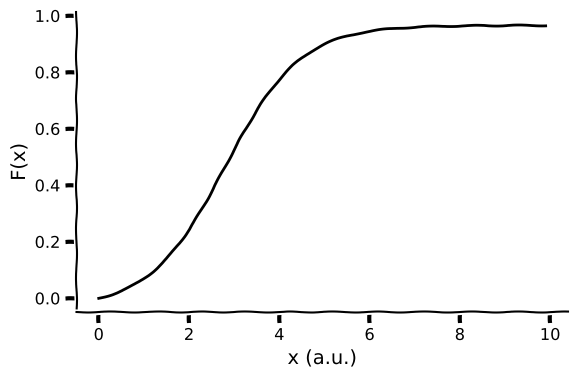
この演習では、ゲインと閾値をパラメータとするシグモイド型のF-I曲線(転送関数)を実装します:
def F(x, a, theta):
  """
  Population activation function.

  Args:
    x (float): the population input
    a (float): the gain of the function
    theta (float): the threshold of the function

  Returns:
    float: the population activation response F(x) for input x
  """
  #################################################
  ## TODO for students: compute f = F(x) ##
  # Fill out function and remove
  raise NotImplementedError("Student exercise: implement the f-I function")
  #################################################

  # Define the sigmoidal transfer function f = F(x)
  f = ...

  return f


# Set parameters
pars = default_pars_single()  # get default parameters
x = np.arange(0, 10, .1)      # set the range of input

# Compute transfer function
f = F(x, pars['a'], pars['theta'])

# Visualize
plot_fI(x, f)出力例:
# @title Submit your feedback
content_review(f"{feedback_prefix}_Implement_FI_curve_Exercise")
インタラクティブデモ 1.2 : F-I曲線のパラメータ探索
ゲインと閾値のパラメータを変えたときにF-I曲線がどう変化するかを示すインタラクティブデモです。
- ゲインパラメータ()はF-I曲線にどのように影響しますか?
- 閾値パラメータ()はF-I曲線にどのように影響しますか?
# @markdown Make sure you execute this cell to enable the widget!

@widgets.interact(
    a=widgets.FloatSlider(1.5, min=0.3, max=3., step=0.3),
    theta=widgets.FloatSlider(3., min=2., max=4., step=0.2)
)


def interactive_plot_FI(a, theta):
  """
  Population activation function.

  Expecxts:
    a     : the gain of the function
    theta : the threshold of the function

  Returns:
    plot the F-I curve with give parameters
  """

  # set the range of input
  x = np.arange(0, 10, .1)
  plt.figure()
  plt.plot(x, F(x, a, theta), 'k')
  plt.xlabel('x (a.u.)', fontsize=14)
  plt.ylabel('F(x)', fontsize=14)
plt.show()# @title Submit your feedback
content_review(f"{feedback_prefix}_Parameter_exploration_of_FI_curve_Interactive_Demo_and_Discussion")セクション1.3: E集団動態のシミュレーションスキーム
チュートリアル開始からここまでの推定時間: 27分
が非線形関数であるため、集団活動の微分方程式の厳密解は解析的に求められません。前に見たように、数値解法、特にオイラー法を使って解(すなわち集団活動)をシミュレートできます。
# @markdown Execute this cell to enable the single population rate model simulator: `simulate_single`


def simulate_single(pars):
  """
  Simulate an excitatory population of neurons

  Args:
    pars   : Parameter dictionary

  Returns:
    rE     : Activity of excitatory population (array)

  Example:
    pars = default_pars_single()
    r = simulate_single(pars)
  """

  # Set parameters
  tau, a, theta = pars['tau'], pars['a'], pars['theta']
  w = pars['w']
  I_ext = pars['I_ext']
  r_init = pars['r_init']
  dt, range_t = pars['dt'], pars['range_t']
  Lt = range_t.size

  # Initialize activity
  r = np.zeros(Lt)
  r[0] = r_init
  I_ext = I_ext * np.ones(Lt)

  # Update the E activity
  for k in range(Lt - 1):
      dr = dt / tau * (-r[k] + F(w * r[k] + I_ext[k], a, theta))
      r[k+1] = r[k] + dr

  return r


help(simulate_single)
インタラクティブデモ 1.3: 単一集団動態のパラメータ探索
このインタラクティブデモで集団活動の動態を探索しましょう。
- の値を変えるとはどう変わりますか?
- の値を変えるとどう変わりますか?
なお、は解析解を示します。次のセクションで計算方法を学びます。
# @title

# @markdown Make sure you execute this cell to enable the widget!

# get default parameters
pars = default_pars_single(T=20.)

@widgets.interact(
    I_ext=widgets.FloatSlider(5.0, min=0.0, max=10., step=1.),
    tau=widgets.FloatSlider(3., min=1., max=5., step=0.2)
)


def Myplot_E_diffI_difftau(I_ext, tau):
  # set external input and time constant
  pars['I_ext'] = I_ext
  pars['tau'] = tau

  # simulation
  r = simulate_single(pars)

  # Analytical Solution
  r_ana = (pars['r_init']
           + (F(I_ext, pars['a'], pars['theta'])
           - pars['r_init']) * (1. - np.exp(-pars['range_t'] / pars['tau'])))

  # plot
  plt.figure()
  plt.plot(pars['range_t'], r, 'b', label=r'$r_{\mathrm{sim}}$(t)', alpha=0.5,
           zorder=1)
  plt.plot(pars['range_t'], r_ana, 'b--', lw=5, dashes=(2, 2),
           label=r'$r_{\mathrm{ana}}$(t)', zorder=2)
  plt.plot(pars['range_t'],
           F(I_ext, pars['a'], pars['theta']) * np.ones(pars['range_t'].size),
           'k--', label=r'$F(I_{\mathrm{ext}})$')
  plt.xlabel('t (ms)', fontsize=16.)
  plt.ylabel('Activity r(t)', fontsize=16.)
  plt.legend(loc='best', fontsize=14.)
plt.show()# @title Submit your feedback
content_review(f"{feedback_prefix}_Parameter_exploration_of_single_population_dynamics_Interactive_Demo_and_Discussion")考えてみよう 1.3: 有界な活動
上記では正の入力で駆動されるシステムを数値的に解きましたが、は0に減衰するか、固定の非ゼロ値に収束します。
- なぜシステムの解は有限時間で「爆発」しないのでしょうか?言い換えれば、が有限に保たれる保証は何でしょうか?
- 応答の最大値を上げるにはどのパラメータを変えればよいでしょうか?
# @title Submit your feedback
content_review(f"{feedback_prefix}_Finite_activities_Discussion")
セクション2: 単一集団システムの固定点
チュートリアル開始からここまでの推定時間: 45分
セクション2.1: 固定点の探索
# @title Video 2: Fixed point
from ipywidgets import widgets
from IPython.display import YouTubeVideo
from IPython.display import IFrame
from IPython.display import display


class PlayVideo(IFrame):
  def __init__(self, id, source, page=1, width=400, height=300, **kwargs):
    self.id = id
    if source == 'Bilibili':
      src = f'https://player.bilibili.com/player.html?bvid={id}&page={page}'
    elif source == 'Osf':
      src = f'https://mfr.ca-1.osf.io/render?url=https://osf.io/download/{id}/?direct%26mode=render'
    super(PlayVideo, self).__init__(src, width, height, **kwargs)


def display_videos(video_ids, W=400, H=300, fs=1):
  tab_contents = []
  for i, video_id in enumerate(video_ids):
    out = widgets.Output()
    with out:
      if video_ids[i][0] == 'Youtube':
        video = YouTubeVideo(id=video_ids[i][1], width=W,
                             height=H, fs=fs, rel=0)
        print(f'Video available at https://youtube.com/watch?v={video.id}')
      else:
        video = PlayVideo(id=video_ids[i][1], source=video_ids[i][0], width=W,
                          height=H, fs=fs, autoplay=False)
        if video_ids[i][0] == 'Bilibili':
          print(f'Video available at https://www.bilibili.com/video/{video.id}')
        elif video_ids[i][0] == 'Osf':
          print(f'Video available at https://osf.io/{video.id}')
      display(video)
    tab_contents.append(out)
  return tab_contents


video_ids = [('Youtube', 'Ox3ELd1UFyo'), ('Bilibili', 'BV1v54y1v7Gr')]
tab_contents = display_videos(video_ids, W=854, H=480)
tabs = widgets.Tab()
tabs.children = tab_contents
for i in range(len(tab_contents)):
  tabs.set_title(i, video_ids[i][0])
display(tabs)
# @title Submit your feedback
content_review(f"{feedback_prefix}_Finding_fixed_points_Video")このビデオでは再帰ネットワークとその固定点の導出方法を紹介します。また、1次元のベクトル場と位相平面も説明します。
ビデオのテキスト要約はこちらをクリック
フィードフォワードネットワークを再帰ネットワークに拡張できます。再帰ネットワークは次の方程式で支配されます:
\begin{align}
&= -r + F(w\cdot r + I_{\text{ext}}) \quad\qquad (3)
\end{align}
ここで、は時刻の興奮性集団の平均発火率、は平均発火率の変化の時間スケール、は外部入力、は全入力に対する集団活性化関数を表します。は集団への再帰入力の強さ(シナプス重み)を示します。
前のインタラクティブデモでパラメータを変えたとき、システムの出力は最初は急速に変化しますが、時間が経つと最大/最小値に達して変化しなくなります。この最終的な値をシステムの定常状態または固定点と呼びます。定常状態では活動の時間微分がゼロ、すなわちです。
式(1)の定常状態はと置いてを解くことで求められます:
この式の解が存在すれば、式(3)の動的システムの固定点を定義します。が非線形の場合、解析解を得るのは難しいですが、後で数値シミュレーションで解を求めます。
また、の値は初期値から定常状態への収束速度に影響することもインタラクティブデモからわかります。
特にの場合、式(1)の解を解析的に計算でき(青の太い破線)、が固定点への収束に果たす役割を次のように示せます:
\displaystyle{r(t) = \big{[}F(I_{\text{ext}};a,\theta) -r(t=0)\big{]} (1-\text{e}^{-\frac{t}{\tau}})} + r(t=0)次に、数値的に固定点を根探索アルゴリズムで計算します。
コーディング演習 2.1.1: 固定点の可視化
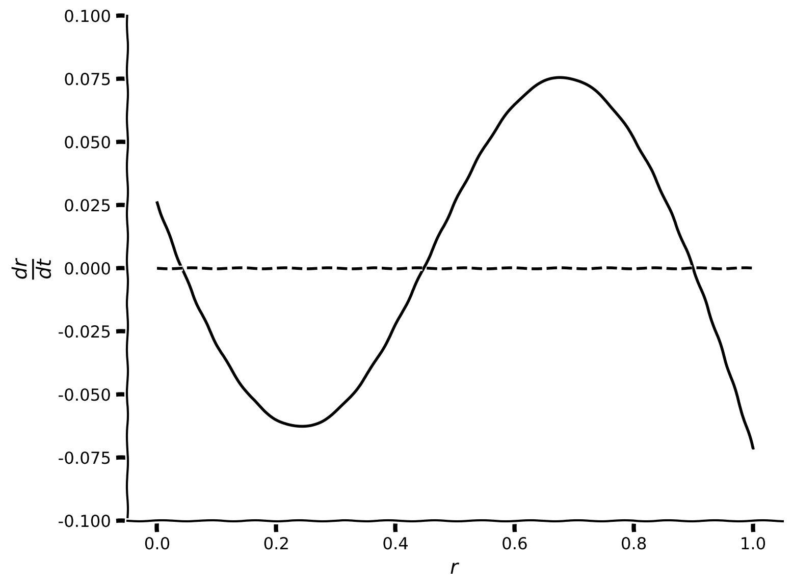
式(3)の解を解析的に求められない場合、グラフ的手法が有効です。そのために、をの関数としてプロットします。y軸でゼロを横切るの値が固定点に対応します。
ここでは例として、とします。式(3)から
を得ます。
これをの関数としてプロットし、固定点の存在を確認してください。
def compute_drdt(r, I_ext, w, a, theta, tau, **other_pars):
  """Given parameters, compute dr/dt as a function of r.

  Args:
    r (1D array) : Average firing rate of the excitatory population
    I_ext, w, a, theta, tau (numbers): Simulation parameters to use
    other_pars : Other simulation parameters are unused by this function

  Returns
    drdt function for each value of r
  """
  #########################################################################
  # TODO compute drdt and disable the error
  raise NotImplementedError("Finish the compute_drdt function")
  #########################################################################

  # Calculate drdt
  drdt = ...

  return drdt


# Define a vector of r values and the simulation parameters
r = np.linspace(0, 1, 1000)
pars = default_pars_single(I_ext=0.5, w=5)

# Compute dr/dt
drdt = compute_drdt(r, **pars)

# Visualize
plot_dr_r(r, drdt)出力例:
# @title Submit your feedback
content_review(f"{feedback_prefix}_Visualization_of_the_fixed_points_Exercise")
コーディング演習 2.1.2: 固定点の数値計算
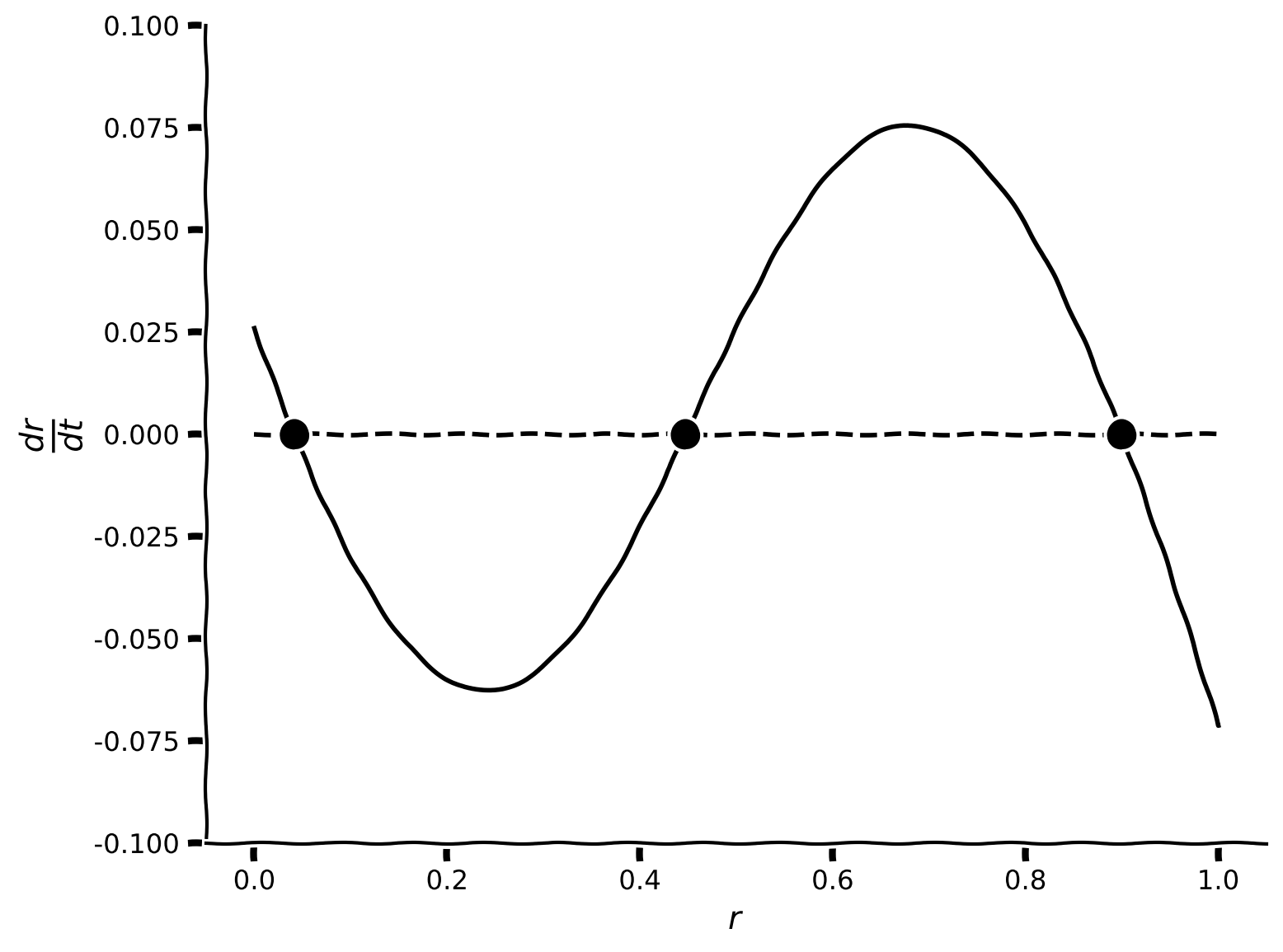
次に固定点を数値的に求めます。根探索アルゴリズムの初期値を指定する必要があります。前の演習でプロットしたの線がy軸のゼロを横切る近傍の値を初期値として選べます。
次のセルでは3つのヘルパー関数を定義しています:
my_fp_single(r_guess, **pars)は根探索アルゴリズムで初期値近傍の固定点を探すcheck_fp_single(x_fp, **pars)はとなるが真の固定点か検証するmy_fp_finder(r_guess_vector, **pars)は初期値の配列を受け取り、上記2関数を使って同数の固定点を見つける
# @markdown Execute this cell to enable the fixed point functions

def my_fp_single(r_guess, a, theta, w, I_ext, **other_pars):
  """
  Calculate the fixed point through drE/dt=0

  Args:
    r_guess  : Initial value used for scipy.optimize function
    a, theta, w, I_ext : simulation parameters

  Returns:
    x_fp    : value of fixed point
  """
  # define the right hand of E dynamics
  def my_WCr(x):
    r = x
    drdt = (-r + F(w * r + I_ext, a, theta))
    y = np.array(drdt)

    return y

  x0 = np.array(r_guess)
  x_fp = opt.root(my_WCr, x0).x.item()

  return x_fp


def check_fp_single(x_fp, a, theta, w, I_ext, mytol=1e-4, **other_pars):
  """
   Verify |dr/dt| < mytol

  Args:
    fp      : value of fixed point
    a, theta, w, I_ext: simulation parameters
    mytol   : tolerance, default as 10^{-4}

  Returns :
    Whether it is a correct fixed point: True/False
  """
  # calculate Equation(3)
  y = x_fp - F(w * x_fp + I_ext, a, theta)

  # Here we set tolerance as 10^{-4}
  return np.abs(y) < mytol


def my_fp_finder(pars, r_guess_vector, mytol=1e-4):
  """
  Calculate the fixed point(s) through drE/dt=0

  Args:
    pars    : Parameter dictionary
    r_guess_vector  : Initial values used for scipy.optimize function
    mytol   : tolerance for checking fixed point, default as 10^{-4}

  Returns:
    x_fps   : values of fixed points

  """
  x_fps = []
  correct_fps = []
  for r_guess in r_guess_vector:
    x_fp = my_fp_single(r_guess, **pars)
    if check_fp_single(x_fp, **pars, mytol=mytol):
      x_fps.append(x_fp)

  return x_fps


help(my_fp_finder)
# Set parameters
r = np.linspace(0, 1, 1000)
pars = default_pars_single(I_ext=0.5, w=5)
# Compute dr/dt
drdt = compute_drdt(r, **pars)
#############################################################################
# TODO for students:
# Define initial values close to the intersections of drdt and y=0
# (How many initial values? Hint: How many times do the two lines intersect?)
# Calculate the fixed point with these initial values and plot them
raise NotImplementedError('student_exercise: find fixed points numerically')
#############################################################################
# Initial guesses for fixed points
r_guess_vector = [...]
# Find fixed point numerically
x_fps = my_fp_finder(pars, r_guess_vector)
# Visualize
plot_dr_r(r, drdt, x_fps)出力例:
# @title Submit your feedback
content_review(f"{feedback_prefix}_Numerical_calculation_of_fixed_points_Exercise")
インタラクティブデモ 2.1: 再帰結合と外部入力に対する固定点
再帰結合と外部入力の値を変えたときに前述のプロットがどのように変化するかを探索できます。固定点の数はどう変わりますか?
# @markdown Make sure you execute this cell to enable the widget!

@widgets.interact(
    w=widgets.FloatSlider(4., min=1., max=7., step=0.2),
    I_ext=widgets.FloatSlider(1.5, min=0., max=3., step=0.1)
)


def plot_intersection_single(w, I_ext):
  # set your parameters
  pars = default_pars_single(w=w, I_ext=I_ext)

  # find fixed points
  r_init_vector = [0, .4, .9]
  x_fps = my_fp_finder(pars, r_init_vector)

  # plot
  r = np.linspace(0, 1., 1000)
  drdt = (-r + F(w * r + I_ext, pars['a'], pars['theta'])) / pars['tau']

plot_dr_r(r, drdt, x_fps)# @title Submit your feedback
content_review(f"{feedback_prefix}_Fixed_points_inputs_Interactive_Demo_and_Discussion")セクション 2.2: 軌道と固定点の関係
時間経過に伴う集団活動と固定点の関係を調べてみましょう。
ここではまず と を設定し、異なる初期値 から始めたときの のダイナミクスを調べます。
# @markdown Execute to visualize dr/dt

def plot_intersection_single(w, I_ext):
  # set your parameters
  pars = default_pars_single(w=w, I_ext=I_ext)

  # find fixed points
  r_init_vector = [0, .4, .9]
  x_fps = my_fp_finder(pars, r_init_vector)

  # plot
  r = np.linspace(0, 1., 1000)
  drdt = (-r + F(w * r + I_ext, pars['a'], pars['theta'])) / pars['tau']

  plot_dr_r(r, drdt, x_fps)


plot_intersection_single(w = 5.0, I_ext = 0.5)
インタラクティブデモ 2.2: 初期値に応じたダイナミクス
このデモで を任意の値に設定してみましょう。解はどのように変化しますか?何を観察しますか?それは前の のプロットとどのように関連していますか?
# @markdown Make sure you execute this cell to enable the widget!
pars = default_pars_single(w=5.0, I_ext=0.5)

@widgets.interact(
    r_init=widgets.FloatSlider(0.5, min=0., max=1., step=.02)
)

def plot_single_diffEinit(r_init):
  pars['r_init'] = r_init
  r = simulate_single(pars)

  plt.figure()
  plt.plot(pars['range_t'], r, 'b', zorder=1)
  plt.plot(0, r[0], 'bo', alpha=0.7, zorder=2)
  plt.xlabel('t (ms)', fontsize=16)
  plt.ylabel(r'$r(t)$', fontsize=16)
  plt.ylim(0, 1.0)
plt.show()# @title Submit your feedback
content_review(f"{feedback_prefix}_Dynamics_initial_value_Interactive_Demo_and_Discussion")の軌道をプロットします。
# @markdown Execute this cell to see the trajectories!

pars = default_pars_single()
pars['w'] = 5.0
pars['I_ext'] = 0.5

plt.figure(figsize=(8, 5))
for ie in range(10):
  pars['r_init'] = 0.1 * ie  # set the initial value
  r = simulate_single(pars)  # run the simulation

  # plot the activity with given initial
  plt.plot(pars['range_t'], r, 'b', alpha=0.1 + 0.1 * ie,
           label=r'r$_{\mathrm{init}}$=%.1f' % (0.1 * ie))

plt.xlabel('t (ms)')
plt.title('Two steady states?')
plt.ylabel(r'$r$(t)')
plt.legend(loc=[1.01, -0.06], fontsize=14)
plt.show()
固定点は3つありますが、現れる定常状態は2つだけです—これはどういうことでしょうか?
実は固定点の安定性が重要です。固定点が安定であれば、その近くから始まった軌道はその固定点の近くに留まり、そこに収束します(定常状態は固定点と等しくなります)。固定点が不安定であれば、その近くから始まった軌道は発散し、安定な固定点に向かいます。実際、不安定な固定点で定常状態に到達する唯一の方法は、初期値が正確にその固定点の値と等しい場合だけです。
考えてみよう 2.2: 安定な固定点と不安定な固定点
このセクションで調べているモデルの固定点のうち、どれが安定でどれが不安定でしょうか?
# @markdown Execute to print fixed point values

# Initial guesses for fixed points
r_guess_vector = [0, .4, .9]

# Find fixed point numerically
x_fps = my_fp_finder(pars, r_guess_vector)

print(f'Our fixed points are {x_fps}')# @title Submit your feedback
content_review(f"{feedback_prefix}_Stable_vs_unstable_fixed_points_Discussion")不安定な固定点から始めた場合の軌道をシミュレーションできます:下の赤い線のように、その固定点に留まることがわかります。
# @markdown Execute to visualize trajectory starting at unstable fixed point
pars = default_pars_single()
pars['w'] = 5.0
pars['I_ext'] = 0.5

plt.figure(figsize=(8, 5))
for ie in range(10):
  pars['r_init'] = 0.1 * ie  # set the initial value
  r = simulate_single(pars)  # run the simulation

  # plot the activity with given initial
  plt.plot(pars['range_t'], r, 'b', alpha=0.1 + 0.1 * ie,
           label=r'r$_{\mathrm{init}}$=%.1f' % (0.1 * ie))

pars['r_init'] = x_fps[1]  # set the initial value
r = simulate_single(pars)  # run the simulation

# plot the activity with given initial
plt.plot(pars['range_t'], r, 'r', alpha=0.1 + 0.1 * ie,
          label=r'r$_{\mathrm{init}}$=%.4f' % (x_fps[1]))

plt.xlabel('t (ms)')
plt.title('Two steady states?')
plt.ylabel(r'$r$(t)')
plt.legend(loc=[1.01, -0.06], fontsize=14)
plt.show()
固定点の安定性を定量的に判定する方法については、ボーナスセクション1を参照してください。
考えてみよう 2: 抑制性集団
このチュートリアルを通じて、、すなわち興奮性ニューロンの単一集団を考えてきました。 を に置き換えた場合、すなわち抑制性ニューロンの集団ではどのような振る舞いになると思いますか?
# @title Submit your feedback
content_review(f"{feedback_prefix}_Inhibitory_populations_Discussion")
まとめ
チュートリアルの推定所要時間:1時間25分
このチュートリアルでは、レートベースの単一ニューロン集団のダイナミクスを調べました。
学んだこと:
- 入力パラメータとネットワークの時定数が集団のダイナミクスに与える影響
- システムの固定点の見つけ方
これらの概念はボーナスマテリアルでさらに発展させています。時間があればぜひご覧ください。そこで学べること:
- システムを線形化して固定点の安定性を判定する方法
- モデルに現実的な入力を加える方法
ボーナス
ボーナスセクション1:動力学の線形化による安定性解析
# @title Video 3: Stability of fixed points
from ipywidgets import widgets
from IPython.display import YouTubeVideo
from IPython.display import IFrame
from IPython.display import display


class PlayVideo(IFrame):
  def __init__(self, id, source, page=1, width=400, height=300, **kwargs):
    self.id = id
    if source == 'Bilibili':
      src = f'https://player.bilibili.com/player.html?bvid={id}&page={page}'
    elif source == 'Osf':
      src = f'https://mfr.ca-1.osf.io/render?url=https://osf.io/download/{id}/?direct%26mode=render'
    super(PlayVideo, self).__init__(src, width, height, **kwargs)


def display_videos(video_ids, W=400, H=300, fs=1):
  tab_contents = []
  for i, video_id in enumerate(video_ids):
    out = widgets.Output()
    with out:
      if video_ids[i][0] == 'Youtube':
        video = YouTubeVideo(id=video_ids[i][1], width=W,
                             height=H, fs=fs, rel=0)
        print(f'Video available at https://youtube.com/watch?v={video.id}')
      else:
        video = PlayVideo(id=video_ids[i][1], source=video_ids[i][0], width=W,
                          height=H, fs=fs, autoplay=False)
        if video_ids[i][0] == 'Bilibili':
          print(f'Video available at https://www.bilibili.com/video/{video.id}')
        elif video_ids[i][0] == 'Osf':
          print(f'Video available at https://osf.io/{video.id}')
      display(video)
    tab_contents.append(out)
  return tab_contents


video_ids = [('Youtube', 'KKMlWWU83Jg'), ('Bilibili', 'BV1oA411e7eg')]
tab_contents = display_videos(video_ids, W=854, H=480)
tabs = widgets.Tab()
tabs.children = tab_contents
for i in range(len(tab_contents)):
  tabs.set_title(i, video_ids[i][0])
display(tabs)
# @title Submit your feedback
content_review(f"{feedback_prefix}_Stability_of_fixed_points_Bonus_Videos")ここでは、固定点の安定性を見極める数学的手法について掘り下げます。
フィードフォワードネットワークの方程式と同様に、一般的な線形システム
は、 で固定点を持ちます。このシステムの解析解は次のように求められます:
ここで、固定点周りの活動に小さな摂動を考えます:、ただし とします。摂動 は時間とともに増大するでしょうか、それとも固定点に収束して減衰するでしょうか? の解析解を用いると、摂動の時間発展は次のように書けます:
-
の場合、 はゼロに減衰し、 は に収束するため、固定点は「安定」です。
-
の場合、 は時間とともに増大し、 は指数関数的に固定点 から離れるため、固定点は「不安定」です。
上記の線形システムと同様に、興奮性集団の動力学の固定点 の安定性を調べるために、方程式 (1) を の周りで だけ摂動し、すなわち とします。方程式 (1) を代入すると、摂動 の時間発展を決定する方程式は次のようになります:
ここで は伝達関数 の微分です。上式は次のように書き換えられます:
つまり、上記の線形システムと同様に、
の値が摂動が増大するかゼロに減衰するかを決定し、すなわち が固定点の安定性を定義します。この値は動的システムの固有値と呼ばれます。
シグモイド型伝達関数の微分は次の通りです:
\begin{align}
& = {-a(x- \
& = a{-a(x-} (1+{-a(x- \qquad (5)
\end{align}
この微分を計算するヘルパー関数 dF を用意しています。
# @markdown Execute this cell to enable helper function `dF` and visualize derivative

def dF(x, a, theta):
  """
  Population activation function.

  Args:
    x     : the population input
    a     : the gain of the function
    theta : the threshold of the function

  Returns:
    dFdx  : the population activation response F(x) for input x
  """

  # Calculate the population activation
  dFdx = a * np.exp(-a * (x - theta)) * (1 + np.exp(-a * (x - theta)))**-2

  return dFdx

# Set parameters
pars = default_pars_single()  # get default parameters
x = np.arange(0, 10, .1)      # set the range of input

# Compute derivative of transfer function
df = dF(x, pars['a'], pars['theta'])

# Visualize
plot_dFdt(x, df)
ボーナスコーディング演習1:固有値を計算しよう
前述の通り、、 の場合、システムは3つの固定点を持ちます。しかし、動力学をシミュレーションし初期条件 を変化させても、2つの定常状態しか得られませんでした。この演習では、関数 eig_single を用いて3つの固定点それぞれの固有値を計算し、安定性を確認します。各固有値の符号(すなわち固定点の安定性)を調べてください。安定な固定点はいくつありますか?
固定点 における固有値の式は次の通りです:
def eig_single(fp, tau, a, theta, w, I_ext, **other_pars):
  """
  Args:
    fp   : fixed point r_fp
    tau, a, theta, w, I_ext : Simulation parameters

  Returns:
    eig : eigenvalue of the linearized system
  """
  #####################################################################
  ## TODO for students: compute eigenvalue and disable the error
  raise NotImplementedError("Student exercise: compute the eigenvalue")
  ######################################################################
  # Compute the eigenvalue
  eig = ...

  return eig


# Find the eigenvalues for all fixed points
pars = default_pars_single(w=5, I_ext=.5)
r_guess_vector = [0, .4, .9]
x_fp = my_fp_finder(pars, r_guess_vector)


for fp in x_fp:
  eig_fp = eig_single(fp, **pars)
  print(f'Fixed point1 at {fp:.3f} with Eigenvalue={eig_fp:.3f}')
実行例
Fixed point1 at 0.042 with Eigenvalue=-0.583
Fixed point2 at 0.447 with Eigenvalue=0.498
Fixed point3 at 0.900 with Eigenvalue=-0.626
# @title Submit your feedback
content_review(f"{feedback_prefix}_Compute_eigenvalues_Bonus_Exercise")
1つ目と3つ目の固定点は安定(固有値が負)、2つ目は不安定(固有値が正)であることがわかります。予想通りですね!
ボーナスセクション2:ノイズ入力が2つの安定状態間の遷移を駆動する
これまでのいくつかのチュートリアルで説明したように、オーンシュタイン・ウーレンベック(OU)過程はニューロンへのノイズ入力を生成するのに一般的に用いられます。OU入力 は次の式に従います:
以下の関数 my_OU(pars, sig, myseed=False) を実行してOU過程を生成してください。
# @markdown Execute to get helper function `my_OU` and visualize OU process


def my_OU(pars, sig, myseed=False):
  """
  A functions that generates Ornstein-Uhlenback process

  Args:
    pars       : parameter dictionary
    sig        : noise amplitute
    myseed     : random seed. int or boolean

  Returns:
    I          : Ornstein-Uhlenbeck input current
  """

  # Retrieve simulation parameters
  dt, range_t = pars['dt'], pars['range_t']
  Lt = range_t.size
  tau_ou = pars['tau_ou']  # [ms]

  # set random seed
  if myseed:
      np.random.seed(seed=myseed)
  else:
      np.random.seed()

  # Initialize
  noise = np.random.randn(Lt)
  I_ou = np.zeros(Lt)
  I_ou[0] = noise[0] * sig

  # generate OU
  for it in range(Lt - 1):
    I_ou[it + 1] = (I_ou[it]
                    + dt / tau_ou * (0. - I_ou[it])
                    + np.sqrt(2 * dt / tau_ou) * sig * noise[it + 1])

  return I_ou


pars = default_pars_single(T=100)
pars['tau_ou'] = 1.  # [ms]
sig_ou = 0.1
I_ou = my_OU(pars, sig=sig_ou, myseed=2020)
plt.figure(figsize=(10, 4))
plt.plot(pars['range_t'], I_ou, 'r')
plt.xlabel('t (ms)')
plt.ylabel(r'$I_{\mathrm{OU}}$')
plt.show()
2つ以上の固定点が存在する場合、ノイズ入力が固定点間の遷移を引き起こすことがあります!ここでは、E集団に対して1,000 ms間OU入力を与えて刺激します。
# @markdown Execute this cell to simulate E population with OU inputs

pars = default_pars_single(T=1000)
pars['w'] = 5.0
sig_ou = 0.7
pars['tau_ou'] = 1.  # [ms]
pars['I_ext'] = 0.56 + my_OU(pars, sig=sig_ou, myseed=2020)

r = simulate_single(pars)

plt.figure(figsize=(10, 4))
plt.plot(pars['range_t'], r, 'b', alpha=0.8)
plt.xlabel('t (ms)')
plt.ylabel(r'$r(t)$')
plt.show()
集団活動が固定点間を行き来している様子(上下に変動している)を見ることができます!