ボーナスチュートリアル：スパイクタイミング依存可塑性（STDP）

第2週4日目：生物学的ニューロンモデル

Neuromatch Academyによる

コンテンツ作成者: Qinglong Gu, Songtin Li, John Murray, Richard Naud, Arvind Kumar

コンテンツレビュアー: Spiros Chavlis, Lorenzo Fontolan, Richard Gao, Matthew Krause

制作編集者: Gagana B, Spiros Chavlis

チュートリアルの目的

このチュートリアルでは、シナプス強度が、シナプス前ニューロンとシナプス後ニューロンのスパイクの相対的なタイミング（すなわち時間差）に応じて変化するシナプスのモデル構築に焦点を当てます。このシナプス重みの変化は**スパイクタイミング依存可塑性（STDP）**として知られています。

このチュートリアルの目標は：

• STDPを示すシナプスのモデルを構築すること

• 入力スパイク列の相関がシナプス重みの分布にどのように影響するかを調べること

これらの目標に向けて、シナプス前入力はポアソン型スパイク列としてモデル化します。シナプス後ニューロンはLIFニューロンとしてモデル化します（チュートリアル1参照）。

このチュートリアル全体を通じて、単一のシナプス後ニューロンが$N$個のシナプス前ニューロンによって駆動されると仮定します。すなわち、$N$個のシナプスがあり、それらの重みが入力スパイク列の統計やシナプス後ニューロンのスパイクとのタイミングにどのように依存するかを調べます。

セットアップ

# @title Install and import feedback gadget


from vibecheck import DatatopsContentReviewContainer
def content_review(notebook_section: str):
    return DatatopsContentReviewContainer(
        "",  # No text prompt
        notebook_section,
        {
            "url": "https://pmyvdlilci.execute-api.us-east-1.amazonaws.com/klab",
            "name": "neuromatch_cn",
            "user_key": "y1x3mpx5",
        },
    ).render()


feedback_prefix = "W2D3_T4_Bonus"

# Import libraries
import matplotlib.pyplot as plt
import numpy as np
import time

# @title Figure Settings
import logging
logging.getLogger('matplotlib.font_manager').disabled = True

import ipywidgets as widgets  # interactive display
%config InlineBackend.figure_format='retina'
# use NMA plot style
plt.style.use("https://raw.githubusercontent.com/NeuromatchAcademy/course-content/main/nma.mplstyle")
my_layout = widgets.Layout()

# @title Plotting functions
def my_raster_plot(range_t, spike_train, n):
  """Generates poisson trains

  Args:
    range_t     : time sequence
    spike_train : binary spike trains, with shape (N, Lt)
    n           : number of Poisson trains plot

  Returns:
    Raster_plot of the spike train
  """

  # Find the number of all the spike trains
  N = spike_train.shape[0]

  # n should be smaller than N:
  if n > N:
    print('The number n exceeds the size of spike trains')
    print('The number n is set to be the size of spike trains')
    n = N

  # Raster plot
  i = 0
  while i <= n:
    if spike_train[i, :].sum() > 0.:
      t_sp = range_t[spike_train[i, :] > 0.5]  # spike times
      plt.plot(t_sp, i * np.ones(len(t_sp)), 'k|', ms=10, markeredgewidth=2)
    i += 1
  plt.xlim([range_t[0], range_t[-1]])
  plt.ylim([-0.5, n + 0.5])
  plt.xlabel('Time (ms)')
  plt.ylabel('Neuron ID')
  plt.show()


def my_example_P(pre_spike_train_ex, pars, P):
  """Generates two plots (raster plot and LTP vs time plot)

  Args:
    pre_spike_train_ex     : spike-train
    pars : dictionary with the parameters
    P : LTP ratio

  Returns:
    my_example_P returns a rastert plot (top),
    and a LTP ratio across time (bottom)
  """
  spT = pre_spike_train_ex
  plt.figure(figsize=(7, 6))
  plt.subplot(211)
  color_set = ['red', 'blue', 'black', 'orange', 'cyan']
  for i in range(spT.shape[0]):
    t_sp = pars['range_t'][spT[i, :] > 0.5]   # spike times
    plt.plot(t_sp, i*np.ones(len(t_sp)), '|',
             color=color_set[i],
             ms=10, markeredgewidth=2)
  plt.xlabel('Time (ms)')
  plt.ylabel('Neuron ID')
  plt.xlim(0, 200)

  plt.subplot(212)
  for k in range(5):
    plt.plot(pars['range_t'], P[k, :], color=color_set[k], lw=1.5)
  plt.xlabel('Time (ms)')
  plt.ylabel('P(t)')
  plt.xlim(0, 200)

  plt.tight_layout()
  plt.show()


def mySTDP_plot(A_plus, A_minus, tau_stdp, time_diff, dW):
  plt.figure()
  plt.plot([-5 * tau_stdp, 5 * tau_stdp], [0, 0], 'k', linestyle=':')
  plt.plot([0, 0], [-A_minus, A_plus], 'k', linestyle=':')

  plt.plot(time_diff[time_diff <= 0], dW[time_diff <= 0], 'ro')
  plt.plot(time_diff[time_diff > 0], dW[time_diff > 0], 'bo')

  plt.xlabel(r't$_{\mathrm{pre}}$ - t$_{\mathrm{post}}$ (ms)')
  plt.ylabel(r'$\Delta$W', fontsize=12)
  plt.title('Biphasic STDP', fontsize=12, fontweight='bold')
  plt.show()

# @title Helper functions

def default_pars_STDP(**kwargs):
  pars = {}

  # typical neuron parameters
  pars['V_th'] = -55.     # spike threshold [mV]
  pars['V_reset'] = -75.  # reset potential [mV]
  pars['tau_m'] = 10.     # membrane time constant [ms]
  pars['V_init'] = -65.   # initial potential [mV]
  pars['V_L'] = -75.      # leak reversal potential [mV]
  pars['tref'] = 2.       # refractory time (ms)

  # STDP parameters
  pars['A_plus'] = 0.008                   # magnitude of LTP
  pars['A_minus'] = pars['A_plus'] * 1.10  # magnitude of LTD
  pars['tau_stdp'] = 20.                   # STDP time constant [ms]

  # simulation parameters
  pars['T'] = 400.  # Total duration of simulation [ms]
  pars['dt'] = .1   # Simulation time step [ms]

  # external parameters if any
  for k in kwargs:
    pars[k] = kwargs[k]

  pars['range_t'] = np.arange(0, pars['T'], pars['dt'])  # Vector of discretized time points [ms]

  return pars


def Poisson_generator(pars, rate, n, myseed=False):
  """Generates poisson trains

  Args:
    pars            : parameter dictionary
    rate            : noise amplitute [Hz]
    n               : number of Poisson trains
    myseed          : random seed. int or boolean

  Returns:
    pre_spike_train : spike train matrix, ith row represents whether
                      there is a spike in ith spike train over time
                      (1 if spike, 0 otherwise)
  """

  # Retrieve simulation parameters
  dt, range_t = pars['dt'], pars['range_t']
  Lt = range_t.size

  # set random seed
  if myseed:
    np.random.seed(seed=myseed)
  else:
    np.random.seed()

  # generate uniformly distributed random variables
  u_rand = np.random.rand(n, Lt)

  # generate Poisson train
  poisson_train = 1. * (u_rand < rate * (dt / 1000.))

  return poisson_train

セクション1：スパイクタイミング依存可塑性（STDP）

# @title Video 1: STDP
from ipywidgets import widgets
from IPython.display import YouTubeVideo
from IPython.display import IFrame
from IPython.display import display


class PlayVideo(IFrame):
  def __init__(self, id, source, page=1, width=400, height=300, **kwargs):
    self.id = id
    if source == 'Bilibili':
      src = f'https://player.bilibili.com/player.html?bvid={id}&page={page}'
    elif source == 'Osf':
      src = f'https://mfr.ca-1.osf.io/render?url=https://osf.io/download/{id}/?direct%26mode=render'
    super(PlayVideo, self).__init__(src, width, height, **kwargs)


def display_videos(video_ids, W=400, H=300, fs=1):
  tab_contents = []
  for i, video_id in enumerate(video_ids):
    out = widgets.Output()
    with out:
      if video_ids[i][0] == 'Youtube':
        video = YouTubeVideo(id=video_ids[i][1], width=W,
                             height=H, fs=fs, rel=0)
        print(f'Video available at https://youtube.com/watch?v={video.id}')
      else:
        video = PlayVideo(id=video_ids[i][1], source=video_ids[i][0], width=W,
                          height=H, fs=fs, autoplay=False)
        if video_ids[i][0] == 'Bilibili':
          print(f'Video available at https://www.bilibili.com/video/{video.id}')
        elif video_ids[i][0] == 'Osf':
          print(f'Video available at https://osf.io/{video.id}')
      display(video)
    tab_contents.append(out)
  return tab_contents


video_ids = [('Youtube', 'luHL-mO5S1w'), ('Bilibili', 'BV1AV411r75K')]
tab_contents = display_videos(video_ids, W=854, H=480)
tabs = widgets.Tab()
tabs.children = tab_contents
for i in range(len(tab_contents)):
  tabs.set_title(i, video_ids[i][0])
display(tabs)

# @title Submit your feedback
content_review(f"{feedback_prefix}_STDP_Video")

STDPのモデル

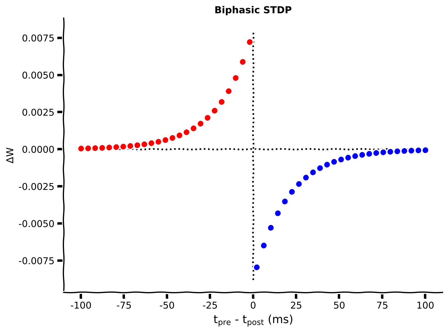
STDPの現象は一般に双相性の指数関数的減衰関数として記述されます。すなわち、重みの瞬時変化は以下のように与えられます：

\begin{eqnarray}
& $\Delta W$ &=& A_+ e^{ ($t_{pre}-t_{post})/$\tau_+} &$\text{if} \hspace{5mm} t_{post} > t_{pre}$& \
& $\Delta W$ &=& -A_- e^{- ($t_{pre}-t_{post})/$\tau_-} &$\text{if} \hspace{5mm} t_{post} < t_{pre}$&
\end{eqnarray}

ここで、$\Delta W$はシナプス重みの変化を示し、$A_+$と$A_-$はシナプス変化の最大値（シナプス前後のスパイクのタイミング差がゼロに近いときに起こる）を決定し、$\tau_+$と$\tau_-$はシナプス強化または弱化が起こるシナプス前後のインタースパイク間隔の範囲を決定します。したがって、$\Delta W > 0$はシナプス後ニューロンがシナプス前ニューロンの後にスパイクすることを意味します。

このモデルは、シナプス後の活動電位の数ミリ秒前にシナプス前スパイクが繰り返し起こるとシナプスの長期増強（LTP）が起こり、シナプス後のスパイク後にシナプス前スパイクが繰り返し起こると同じシナプスの長期抑圧（LTD）が起こる現象を捉えています。

シナプス前後のスパイク間の遅延（$\Delta t$）は以下のように定義されます：

ここで、$t_{\rm pre}$と$t_{\rm post}$はそれぞれシナプス前とシナプス後のスパイクのタイミングです。

以下のコードを完成させてSTDPパラメータを設定し、STDP関数をプロットしてください。簡単のために、**$\tau_{+} = \tau_{-} = \tau_{\rm stdp}$**と仮定します。

コーディング演習1A：STDP変化量$\Delta W$の計算

上記のように、$\Delta W$の式は$t_{post}>t_{pre}$と$t_{post}<t_{pre}$で異なります。コードでは、$t_{pre}-t_{post}$を表すパラメータtime_diffを使用します。

コードを実装した後、STDPカーネルを可視化できます。これは、シナプス前後のスパイク間の遅延に応じてシナプス重みがどの程度変化するかを示します。

def Delta_W(pars, A_plus, A_minus, tau_stdp):
  """
  Plot STDP biphasic exponential decaying function

  Args:
    pars       : parameter dictionary
    A_plus     : (float) maximum amount of synaptic modification
                 which occurs when the timing difference between pre- and
                 post-synaptic spikes is positive
    A_minus    : (float) maximum amount of synaptic modification
                 which occurs when the timing difference between pre- and
                 post-synaptic spikes is negative
    tau_stdp   : the ranges of pre-to-postsynaptic interspike intervals
                 over which synaptic strengthening or weakening occurs

  Returns:
    dW         : instantaneous change in weights
  """
  #######################################################################
  ## TODO for students: compute dP, then remove the NotImplementedError #
  # Fill out when you finish the function
  raise NotImplementedError("Student exercise: compute dW, the change in weights!")
  #######################################################################
  # STDP change
  dW = np.zeros(len(time_diff))
  # Calculate dW for LTP
  dW[time_diff <= 0] = ...
  # Calculate dW for LTD
  dW[time_diff > 0] = ...

  return dW


pars = default_pars_STDP()
# Get parameters
A_plus, A_minus, tau_stdp = pars['A_plus'], pars['A_minus'], pars['tau_stdp']
# pre_spike time - post_spike time
time_diff = np.linspace(-5 * tau_stdp, 5 * tau_stdp, 50)

dW = Delta_W(pars, A_plus, A_minus, tau_stdp)
mySTDP_plot(A_plus, A_minus, tau_stdp, time_diff, dW)

解答を見る$

出力例:

# @title Submit your feedback
content_review(f"{feedback_prefix}_Compute_STDP_changes_Exercise")

シナプス前後のスパイクの追跡

ニューロンは多数のシナプス前スパイク入力を受けるため、異なるシナプスを考慮してSTDPを実装するには、シミュレーション中にシナプス前後のスパイク時刻を追跡する必要があります。

便利な方法として、各シナプス後ニューロンに対して以下の方程式を定義します：

そしてシナプス後ニューロンがスパイクするたびに、

このようにして$M(t)$は時定数$\tau_{-}$のスケールでシナプス後スパイクの数を追跡します。

同様に、各シナプス前ニューロンに対しては：

そしてシナプス前ニューロンにスパイクがあるたびに、

変数$M(t)$と$P(t)$はシナプスコンダクタンス$g_{i}(t)$の方程式に似ていますが、はるかに長い時間スケールでシナプス前後のスパイク時刻を追跡するために使われます。$M(t)$は常に負で、$P(t)$は常に正です。$M$はLTDを誘導し、$P$はLTPを誘導するためにそれぞれ$A_{-}$と$A_{+}$で更新されることは想像できるでしょう。

重要な注意: $P(t)$はシナプス前スパイク時刻に依存します。シナプス前スパイク時刻がわかれば、$P$はシナプス後ニューロンのシミュレーション前に生成でき、対応するSTDP重みも計算できます。

$P$の可視化

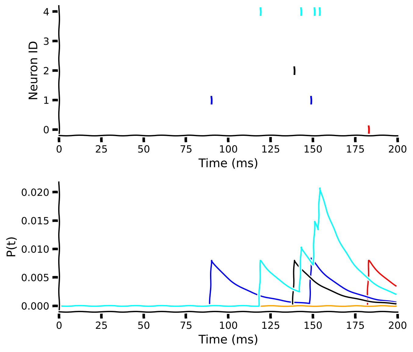
ここでは、単一のシナプス後ニューロンが$N$個のシナプス前ニューロンに接続されているシナリオを考えます。

例えば、1つのシナプス後ニューロンが5つのシナプス前ニューロンからのポアソン型スパイク入力を受けています。

各シナプス前ニューロンについて$P$をシミュレートできます。

コーディング演習1B：$dP$の計算

ここでも、前のチュートリアルで何度も紹介したオイラー法を使います。

LIFモデルの膜電位の動力学と同様に、時間ステップ$dt$で$P(t)$は$\displaystyle{\frac{dt}{\tau_+}P(t)}$だけ減少します。一方、シナプス前スパイクが到着すると$P(t)$は瞬時に$A_+$だけ増加します。したがって、

ここで\text{sp_or_not}はバイナリ変数で、$dt$内にスパイクがあれば1、なければ0です。

def generate_P(pars, pre_spike_train_ex):
  """
  track of pre-synaptic spikes

  Args:
    pars               : parameter dictionary
    pre_spike_train_ex : binary spike train input from
                         presynaptic excitatory neuron

  Returns:
    P                  : LTP ratio
  """

  # Get parameters
  A_plus, tau_stdp = pars['A_plus'], pars['tau_stdp']
  dt, range_t = pars['dt'], pars['range_t']
  Lt = range_t.size

  # Initialize
  P = np.zeros(pre_spike_train_ex.shape)
  for it in range(Lt - 1):
    #######################################################################
    ## TODO for students: compute dP, then remove the NotImplementedError #
    # Fill out when you finish the function
    raise NotImplementedError("Student exercise: compute P, the change of presynaptic spike")
    #######################################################################
    # Calculate the delta increment dP
    dP = ...
    # Update P
    P[:, it + 1] = P[:, it] + dP

  return P


pars = default_pars_STDP(T=200., dt=1.)
pre_spike_train_ex = Poisson_generator(pars, rate=10, n=5, myseed=2020)
P = generate_P(pars, pre_spike_train_ex)
my_example_P(pre_spike_train_ex, pars, P)

解答を見る$

出力例:

# @title Submit your feedback
content_review(f"{feedback_prefix}_Compute_dP_Exercise")

セクション2：STDPの実装

最後に、スパイキングネットワークでSTDPを実装するために、シナプス前後のタイミングに基づいてピークシナプスコンダクタンスの値を変化させ、変数$P(t)$と$M(t)$を使います。

各シナプス$i$はそれぞれピークシナプスコンダクタンス($\bar g_i$)を持ち、これは$[0, \bar g_{max}]$の範囲で変動し、シナプス前後のタイミングに応じて変化します。

• $i$番目のシナプス前ニューロンがスパイクを発生させると、その対応するピークコンダクタンスは以下の式で更新されます：

  $$$$

\bar g_i = \bar g_i + P_i(t)\bar g_{max}, \forall i

STDPを示すシナプスに接続されたLIFニューロン

次の演習では、$N$個のシナプス前ニューロンを単一のシナプス後ニューロンに接続します。スパイク時刻のみ関心があるため、各シナプス前ニューロンの動力学はシミュレートしません。代わりに$N$個のポアソン型スパイクを生成します。ここでは、すべての入力が興奮性であると仮定します。

シナプス後ニューロンのスパイク時刻は未知なので、その動力学はシミュレートする必要があります。シナプス後ニューロンは興奮性入力のみを受けるLIFニューロンとしてモデル化します。

ここで、総興奮性シナプスコンダクタンス$g_{E}(t)$は以下のように与えられます：

STDPをシミュレートする際は、$\bar g_i$がその範囲を超えないように注意することが重要です。

# @title Function for LIF neuron with STDP synapses

def run_LIF_cond_STDP(pars, pre_spike_train_ex):
  """
  conductance-based LIF dynamics

  Args:
    pars               : parameter dictionary
    pre_spike_train_ex : spike train input from presynaptic excitatory neuron

  Returns:
    rec_spikes         : spike times
    rec_v              : mebrane potential
    gE                 : postsynaptic excitatory conductance
  """

  # Retrieve parameters
  V_th, V_reset = pars['V_th'], pars['V_reset']
  tau_m = pars['tau_m']
  V_init, V_L = pars['V_init'], pars['V_L']
  gE_bar, VE, tau_syn_E = pars['gE_bar'], pars['VE'], pars['tau_syn_E']
  gE_init = pars['gE_init']
  tref = pars['tref']
  A_minus, tau_stdp = pars['A_minus'], pars['tau_stdp']
  dt, range_t = pars['dt'], pars['range_t']
  Lt = range_t.size

  P = generate_P(pars, pre_spike_train_ex)

  # Initialize
  tr = 0.
  v = np.zeros(Lt)
  v[0] = V_init
  M = np.zeros(Lt)
  gE = np.zeros(Lt)
  gE_bar_update = np.zeros(pre_spike_train_ex.shape)
  gE_bar_update[:, 0] = gE_init  # note: gE_bar is the maximum value

  # simulation
  rec_spikes = []  # recording spike times
  for it in range(Lt - 1):
      if tr > 0:
          v[it] = V_reset
          tr = tr - 1
      elif v[it] >= V_th:   # reset voltage and record spike event
          rec_spikes.append(it)
          v[it] = V_reset
          M[it] = M[it] - A_minus
          gE_bar_update[:, it] = gE_bar_update[:, it] + P[:, it] * gE_bar
          id_temp = gE_bar_update[:, it] > gE_bar
          gE_bar_update[id_temp, it] = gE_bar
          tr = tref / dt

      # update the synaptic conductance
      M[it + 1] = M[it] - dt / tau_stdp * M[it]
      gE[it + 1] = gE[it] - (dt / tau_syn_E) * gE[it] + (gE_bar_update[:, it] * pre_spike_train_ex[:, it]).sum()
      gE_bar_update[:, it + 1] = gE_bar_update[:, it] + M[it]*pre_spike_train_ex[:, it]*gE_bar
      id_temp = gE_bar_update[:, it + 1] < 0
      gE_bar_update[id_temp, it + 1] = 0.

      # calculate the increment of the membrane potential
      dv = (-(v[it] - V_L) - gE[it + 1] * (v[it] - VE)) * (dt / tau_m)

      # update membrane potential
      v[it + 1] = v[it] + dv

  rec_spikes = np.array(rec_spikes) * dt

  return v, rec_spikes, gE, P, M, gE_bar_update

print(help(run_LIF_cond_STDP))

興奮性シナプスコンダクタンスの変化

以下では、$N=300$個のシナプス前ニューロンから入力を受けるLIFニューロンをシミュレートします。

pars = default_pars_STDP(T=200., dt=1.)  # Simulation duration 200 ms
pars['gE_bar'] = 0.024                   # max synaptic conductance
pars['gE_init'] = 0.024                  # initial synaptic conductance
pars['VE'] = 0.                          # [mV] Synapse reversal potential
pars['tau_syn_E'] = 5.                   # [ms] EPSP time constant

# generate Poisson type spike trains
pre_spike_train_ex = Poisson_generator(pars, rate=10, n=300, myseed=2020)
# simulate the LIF neuron and record the synaptic conductance
v, rec_spikes, gE, P, M, gE_bar_update = run_LIF_cond_STDP(pars,
                                                           pre_spike_train_ex)

# @title Figures of the evolution of synaptic conductance

# @markdown Run this cell to see the figures!
plt.figure(figsize=(12., 8))
plt.subplot(321)
dt, range_t = pars['dt'], pars['range_t']
if rec_spikes.size:
  sp_num = (rec_spikes / dt).astype(int) - 1
  v[sp_num] += 10   # add artificial spikes
plt.plot(pars['range_t'], v, 'k')
plt.xlabel('Time (ms)')
plt.ylabel('V (mV)')

plt.subplot(322)
# Plot the sample presynaptic spike trains
my_raster_plot(pars['range_t'], pre_spike_train_ex, 10)

plt.subplot(323)
plt.plot(pars['range_t'], M, 'k')
plt.xlabel('Time (ms)')
plt.ylabel('M')

plt.subplot(324)
for i in range(10):
  plt.plot(pars['range_t'], P[i, :])
plt.xlabel('Time (ms)')
plt.ylabel('P')

plt.subplot(325)
for i in range(10):
  plt.plot(pars['range_t'], gE_bar_update[i, :])
plt.xlabel('Time (ms)')
plt.ylabel(r'$\bar g$')

plt.subplot(326)
plt.plot(pars['range_t'], gE, 'r')
plt.xlabel('Time (ms)')
plt.ylabel(r'$g_E$')

plt.tight_layout()
plt.show()

考えてみよう！2A：シナプス強度とコンダクタンスの変化の解析

• 上記では、すべてのシナプス前ニューロンが同じ平均発火率であるにもかかわらず、多くのシナプスが弱化しているように見えます。これは予想通りでしたか？

• 総シナプスコンダクタンスは時間とともに変動しています。もしシナプスがSTDPのような挙動を示さなければ、$g_E$はどのように変動すると予想しますか？

• シナプスがSTDPを示す場合、シナプス重みは定常状態に達することがありますか？

解答を見る$

# @title Submit your feedback
content_review(f"{feedback_prefix}_Analyzing_synaptic_strength_Discussion")

シナプス重みの分布

上記の例から、一部のシナプスは脱増強されることがわかりましたが、STDPを示すシナプスのシナプス重みの分布はどうなっているでしょうか？

実際、シナプス重みの分布自体も時間変動する可能性があります。そこで、シナプス重みの分布が時間とともにどのように変化するかを知りたいです。

重み分布とその時間変化のより良い推定のために、シナプス前発火率を15Hzに上げ、シナプス後ニューロンを120秒間シミュレートします。

# @title Functions for simulating a LIF neuron with STDP synapses


def example_LIF_STDP(inputrate=15., Tsim=120000.):
  """
  Simulation of a LIF model with STDP synapses

  Args:
    intputrate  :  The rate used for generate presynaptic spike trains
    Tsim        :  Total simulation time

  output:
    Interactive demo, Visualization of synaptic weights
  """

  pars = default_pars_STDP(T=Tsim,  dt=1.)
  pars['gE_bar'] = 0.024
  pars['gE_init'] = 0.014  # initial synaptic conductance
  pars['VE'] = 0.          # [mV]
  pars['tau_syn_E'] = 5.   # [ms]

  starttime = time.perf_counter()
  pre_spike_train_ex = Poisson_generator(pars, rate=inputrate, n=300,
                                         myseed=2020)  # generate Poisson trains
  v, rec_spikes, gE, P, M, gE_bar_update = run_LIF_cond_STDP(pars,
                                                             pre_spike_train_ex)  # simulate LIF neuron with STDP
  gbar_norm = gE_bar_update/pars['gE_bar']  # calculate the ratio of the synaptic conductance
  endtime = time.perf_counter()
  timecost = (endtime - starttime) / 60.

  print('Total simulation time is %.3f min' % timecost)

  my_layout.width = '620px'

  @widgets.interact(
      sample_time=widgets.FloatSlider(0.5, min=0., max=1., step=0.1,
                                      layout=my_layout)
  )


  def my_visual_STDP_distribution(sample_time=0.0):
    sample_time = int(sample_time * pars['range_t'].size) - 1
    sample_time = sample_time * (sample_time > 0)

    plt.figure(figsize=(8, 8))
    ax1 = plt.subplot(211)
    for i in range(50):
      ax1.plot(pars['range_t'][::1000] / 1000., gE_bar_update[i, ::1000], lw=1., alpha=0.7)

    ax1.axvline(1e-3 * pars['range_t'][sample_time], 0., 1., color='k', ls='--')
    ax1.set_ylim(0, 0.025)
    ax1.set_xlim(-2, 122)
    ax1.set_xlabel('Time (s)')
    ax1.set_ylabel(r'$\bar{g}$')

    bins = np.arange(-.05, 1.05, .05)
    g_dis, _ = np.histogram(gbar_norm[:, sample_time], bins)
    ax2 = plt.subplot(212)
    ax2.bar(bins[1:], g_dis, color='b', alpha=0.5, width=0.05)
    ax2.set_xlim(-0.1, 1.1)
    ax2.set_xlabel(r'$\bar{g}/g_{\mathrm{max}}$')
    ax2.set_ylabel('Number')
    ax2.set_title(('Time = %.1f s' % (1e-3 * pars['range_t'][sample_time])),
                  fontweight='bold')
    plt.show()


print(help(example_LIF_STDP))

インタラクティブデモ2：STDPを持つLIFモデルの例

# @markdown Make sure you execute this cell to enable the widget!
example_LIF_STDP(inputrate=15)

考えてみよう！2B：シナプス前発火率増加の影響

シナプス前ニューロンの発火率（例えば30Hz）を増加させ、シナプス重み分布の動態に与える影響を調べてみましょう。

解答を見る$

# @title Submit your feedback
content_review(f"{feedback_prefix}_LIF_and_STDP_Interactive_Demo_and_Discussion")

セクション3：入力相関の影響

これまで、入力集団は無相関であると仮定してきました。もしシナプス前ニューロンが相関していたらどうなると思いますか？

以下では、最初の$L$個のニューロンが同一のスパイク列を持ち、残りの入力は無相関であるように入力を変更します。これは相関を導入する非常に単純化したモデルです。自分で相関スパイク列のモデルをコーディングしてみてもよいでしょう。

# @title Function for LIF neuron with STDP synapses receiving correlated inputs


def example_LIF_STDP_corrInput(inputrate=20., Tsim=120000.):
  """
  A LIF model equipped with STDP synapses, receiving correlated inputs

  Args:
    intputrate      :  The rate used for generate presynaptic spike trains
    Tsim            :  Total simulation time

  Returns:
    Interactive demo: Visualization of synaptic weights
  """

  np.random.seed(2020)
  pars = default_pars_STDP(T=Tsim, dt=1.)
  pars['gE_bar'] = 0.024
  pars['VE'] = 0.                                # [mV]
  pars['gE_init'] = 0.024 * np.random.rand(300)  # initial synaptic conductance
  pars['tau_syn_E'] = 5.                         # [ms]

  starttime = time.perf_counter()
  pre_spike_train_ex = Poisson_generator(pars, rate=inputrate, n=300, myseed=2020)
  for i_pre in range(50):
    pre_spike_train_ex[i_pre, :] = pre_spike_train_ex[0, :]  # simple way to set input correlated
  v, rec_spikes, gE, P, M, gE_bar_update = run_LIF_cond_STDP(pars, pre_spike_train_ex) # simulate LIF neuron with STDP
  gbar_norm = gE_bar_update / pars['gE_bar']  # calculate the ratio of the synaptic conductance
  endtime = time.perf_counter()
  timecost = (endtime - starttime) / 60.

  print(f'Total simulation time is {timecost:.3f} min')

  my_layout.width = '620px'

  @widgets.interact(
      sample_time=widgets.FloatSlider(0.5, min=0., max=1., step=0.05,
                                      layout=my_layout)
  )


  def my_visual_STDP_distribution(sample_time=0.0):

    sample_time = int(sample_time * pars['range_t'].size) - 1
    sample_time = sample_time*(sample_time > 0)
    figtemp = plt.figure(figsize=(8, 8))
    ax1 = plt.subplot(211)
    for i in range(50):
      ax1.plot(pars['range_t'][::1000] / 1000.,
               gE_bar_update[i, ::1000], lw=1., color='r', alpha=0.7, zorder=2)

    for i in range(50):
      ax1.plot(pars['range_t'][::1000] / 1000.,
               gE_bar_update[i + 50, ::1000], lw=1., color='b',
               alpha=0.5, zorder=1)

    ax1.axvline(1e-3 * pars['range_t'][sample_time], 0., 1.,
                color='k', ls='--', zorder=2)
    ax1.set_ylim(0, 0.025)
    ax1.set_xlim(-2, 122)
    ax1.set_xlabel('Time (s)')
    ax1.set_ylabel(r'$\bar{g}$')
    legend=ax1.legend(['Correlated input', 'Uncorrelated iput'], fontsize=18,
                      loc=[0.92, -0.6], frameon=False)
    for color, text, item in zip(['r', 'b'], legend.get_texts(), legend.legend_handles):
      text.set_color(color)
      item.set_visible(False)

    bins = np.arange(-.05, 1.05, .05)
    g_dis_cc, _ = np.histogram(gbar_norm[:50, sample_time], bins)
    g_dis_dp, _ = np.histogram(gbar_norm[50:, sample_time], bins)

    ax2 = plt.subplot(212)
    ax2.bar(bins[1:], g_dis_cc, color='r', alpha=0.5, width=0.05)
    ax2.bar(bins[1:], g_dis_dp, color='b', alpha=0.5, width=0.05)
    ax2.set_xlim(-0.1, 1.1)
    ax2.set_xlabel(r'$\bar{g}/g_{\mathrm{max}}$')
    ax2.set_ylabel('Number')
    ax2.set_title(('Time = %.1f s' % (1e-3 * pars['range_t'][sample_time])),
                  fontweight='bold')
    plt.show()


print(help(example_LIF_STDP_corrInput))

インタラクティブデモ3：相関入力を受ける可塑性シナプスを持つLIFモデル

# @markdown Make sure you execute this cell to enable the widget!
example_LIF_STDP_corrInput(inputrate=10.0)

なぜSTDPを示すシナプスで無相関ニューロンの重みが減少するのか？

上記では、相関したニューロン（同時にスパイクする）がほとんど影響を受けなかった一方で、他のニューロンの重みは減少しました。なぜでしょうか？

理由は、相関したシナプス前ニューロンはシナプス後ニューロンのスパイクを誘発する確率が高くなり、$pre \rightarrow post$のスパイクペアリングが生じるためです。

考えてみよう！3：STDPの応用

• 上記のコードを修正して、2つの相関したシナプス前ニューロングループを作り、重み分布がどうなるか試してみましょう。

• 上記の観察結果は教師なし学習を作るためにどのように使えるでしょうか？STDPルールを持つニューロンモデルをどのように訓練して入力パターンを識別させるか想像できますか？

• このタイプの可塑性で他に何ができるでしょうか？

解答を見る$

# @title Submit your feedback
content_review(f"{feedback_prefix}_LIF_plasticity_correlated_inputs_Interactive_Demo_and_Discussion")

まとめ

お疲れさまでした！この長い1日を終えましたね！このチュートリアルでは、**スパイクタイミング依存可塑性（STDP）**の概念を扱いました。

以下を達成しました：

• STDPを示すシナプスのモデルを構築しました。

• 入力スパイク列の相関がシナプス重みの分布にどのように影響するかを調べました。

ポアソン型スパイク列をシナプス前入力として用い、STDPを備えたシナプスを持つLIFモデルを構築しました。また、相関入力がシナプス強度に与える影響も調べました！