チュートリアル 3: シナプス伝達 - 静的および動的シナプスのモデル

第2週、第4日目：生物学的ニューロンモデル

Neuromatch Academyによる

コンテンツ作成者: Qinglong Gu, Songtin Li, John Murray, Richard Naud, Arvind Kumar

コンテンツレビュアー: Maryam Vaziri-Pashkam, Ella Batty, Lorenzo Fontolan, Richard Gao, Matthew Krause, Spiros Chavlis, Michael Waskom

ポストプロダクションチーム: Gagana B, Spiros Chavlis

チュートリアルの目的

推定所要時間：1時間10分

シナプスはニューロンを神経ネットワークや回路に接続します。特殊な電気的シナプスはニューロン間に直接的かつ物理的な接続を作ります。しかし、このチュートリアルでは、脳内でより一般的な化学的シナプスに焦点を当てます。これらのシナプスはニューロンを物理的に結合しません。代わりに、シナプス前細胞のスパイクが神経伝達物質をシナプス間隙と呼ばれるニューロン間の小さな空間に放出させます。この化学物質がその空間を拡散すると、シナプス後膜の透過性が変化し、膜電位に正または負の変化をもたらすことがあります。

このチュートリアルでは、化学的シナプス伝達をモデル化し、静的シナプスと動的シナプスによって生じる興味深い効果を学びます。

まず、重みが常に固定されている静的シナプスのシミュレーションコードを書きます。
次にモデルを拡張し、最近のスパイク履歴に依存してシナプス強度が変化する動的シナプスをモデル化します。シナプスは、シナプス前細胞の最近の発火率に基づいて、シナプス後ニューロンへの影響の大きさを段階的に増加または減少させることができます。この脳内シナプスの特徴は短期可塑性と呼ばれ、促進または抑制を引き起こします。

このチュートリアルの目標は：

静的シナプスをシミュレーションし、興奮性および抑制性がニューロンのスパイク出力パターンにどのように影響するかを調べる
平均駆動または変動駆動の状態を定義する
シナプスの短期動態（促進と抑制）をシミュレーションする
シナプス前の発火履歴の変化がシナプス重み（すなわちPSP振幅）にどのように影響するかを調べる

# @title Tutorial slides
# @markdown These are the slides for the videos in all tutorials today
from IPython.display import IFrame
link_id = "8djsm"
print(f"If you want to download the slides: https://osf.io/download/{link_id}/")
IFrame(src=f"https://mfr.ca-1.osf.io/render?url=https://osf.io/{link_id}/?direct%26mode=render%26action=download%26mode=render", width=854, height=480)

セットアップ

# @title Install and import feedback gadget


from vibecheck import DatatopsContentReviewContainer
def content_review(notebook_section: str):
    return DatatopsContentReviewContainer(
        "",  # No text prompt
        notebook_section,
        {
            "url": "https://pmyvdlilci.execute-api.us-east-1.amazonaws.com/klab",
            "name": "neuromatch_cn",
            "user_key": "y1x3mpx5",
        },
    ).render()


feedback_prefix = "W2D3_T3"

# Imports
import matplotlib.pyplot as plt
import numpy as np

# @title Figure Settings
import logging
logging.getLogger('matplotlib.font_manager').disabled = True

import ipywidgets as widgets  # interactive display
%config InlineBackend.figure_format='retina'
# use NMA plot style
plt.style.use("https://raw.githubusercontent.com/NeuromatchAcademy/course-content/main/nma.mplstyle")
my_layout = widgets.Layout()

# @title Plotting Functions

def my_illus_LIFSYN(pars, v_fmp, v):
  """
  Illustartion of FMP and membrane voltage

  Args:
    pars  : parameters dictionary
    v_fmp : free membrane potential, mV
    v     : membrane voltage, mV

  Returns:
    plot of membrane voltage and FMP, alongside with the spiking threshold
    and the mean FMP (dashed lines)
  """

  plt.figure(figsize=(14, 5))
  plt.plot(pars['range_t'], v_fmp, 'r', lw=1.,
           label='Free mem. pot.', zorder=2)
  plt.plot(pars['range_t'], v, 'b', lw=1.,
           label='True mem. pot', zorder=1, alpha=0.7)
  plt.axhline(pars['V_th'], 0, 1, color='k', lw=2., ls='--',
              label='Spike Threshold', zorder=1)
  plt.axhline(np.mean(v_fmp), 0, 1, color='r', lw=2., ls='--',
              label='Mean Free Mem. Pot.', zorder=1)
  plt.xlabel('Time (ms)')
  plt.ylabel('V (mV)')
  plt.legend(loc=[1.02, 0.68])
  plt.show()


def plot_volt_trace(pars, v, sp, show=True):
  """
  Plot trajetory of membrane potential for a single neuron

  Args:
    pars   : parameter dictionary
    v      : volt trajetory
    sp     : spike train

  Returns:
    figure of the membrane potential trajetory for a single neuron
  """

  V_th = pars['V_th']
  dt = pars['dt']
  if sp.size:
    sp_num = (sp/dt).astype(int) - 1
    v[sp_num] += 10

  plt.plot(pars['range_t'], v, 'b')
  plt.axhline(V_th, 0, 1, color='k', ls='--', lw=1.)
  plt.xlabel('Time (ms)')
  plt.ylabel('V (mV)')
  if show:
    plt.show()


def my_illus_STD(Poisson=False, rate=20., U0=0.5,
                 tau_d=100., tau_f=50., plot_out=True):
  """
   Only for one presynaptic train

  Args:
    Poisson    : Poisson or regular input spiking trains
    rate       : Rate of input spikes, Hz
    U0         : synaptic release probability at rest
    tau_d      : synaptic depression time constant of x [ms]
    tau_f      : synaptic facilitation time constantr of u [ms]
    plot_out   : whether ot not to plot, True or False

  Returns:
    Nothing.
  """

  T_simu = 10.0 * 1000 / (1.0 * rate)  # 10 spikes in the time window
  pars = default_pars(T=T_simu)
  dt = pars['dt']

  if Poisson:
    # Poisson type spike train
    pre_spike_train = Poisson_generator(pars, rate, n=1)
    pre_spike_train = pre_spike_train.sum(axis=0)
  else:
    # Regular firing rate
    isi_num = int((1e3/rate)/dt)  # number of dt
    pre_spike_train = np.zeros(len(pars['range_t']))
    pre_spike_train[::isi_num] = 1.

  u, R, g = dynamic_syn(g_bar=1.2, tau_syn=5., U0=U0,
                        tau_d=tau_d, tau_f=tau_f,
                        pre_spike_train=pre_spike_train,
                        dt=pars['dt'])

  if plot_out:
    plt.figure(figsize=(12, 6))

    plt.subplot(221)
    plt.plot(pars['range_t'], R, 'b', label='R')
    plt.plot(pars['range_t'], u, 'r', label='u')
    plt.legend(loc='best')
    plt.xlim((0, pars['T']))
    plt.ylabel(r'$R$ or $u$ (a.u)')
    plt.subplot(223)
    spT = pre_spike_train > 0
    t_sp = pars['range_t'][spT]  #spike times
    plt.plot(t_sp, 0. * np.ones(len(t_sp)), 'k|', ms=18, markeredgewidth=2)
    plt.xlabel('Time (ms)');
    plt.xlim((0, pars['T']))
    plt.yticks([])
    plt.title('Presynaptic spikes')

    plt.subplot(122)
    plt.plot(pars['range_t'], g, 'r', label='STP synapse')
    plt.xlabel('Time (ms)')
    plt.ylabel('g (nS)')
    plt.xlim((0, pars['T']))

    plt.tight_layout()
    plt.show()

  if not Poisson:
    return g[isi_num], g[9*isi_num]

# @title Helper Functions

def my_GWN(pars, mu, sig, myseed=False):
  """
  Args:
    pars       : parameter dictionary
    mu         : noise baseline (mean)
    sig        : noise amplitute (standard deviation)
    myseed     : random seed. int or boolean
                  the same seed will give the same random number sequence

  Returns:
    I          : Gaussian White Noise (GWN) input
  """

  # Retrieve simulation parameters
  dt, range_t = pars['dt'], pars['range_t']
  Lt = range_t.size

  # set random seed
  # you can fix the seed of the random number generator so that the results
  # are reliable. However, when you want to generate multiple realizations
  # make sure that you change the seed for each new realization.
  if myseed:
      np.random.seed(seed=myseed)
  else:
      np.random.seed()

  # generate GWN
  # we divide here by 1000 to convert units to seconds.
  I_GWN = mu + sig * np.random.randn(Lt) / np.sqrt(dt / 1000.)

  return I_GWN


def Poisson_generator(pars, rate, n, myseed=False):
  """
  Generates poisson trains

  Args:
    pars       : parameter dictionary
    rate       : noise amplitute [Hz]
    n          : number of Poisson trains
    myseed     : random seed. int or boolean

  Returns:
    pre_spike_train : spike train matrix, ith row represents whether
                      there is a spike in ith spike train over time
                      (1 if spike, 0 otherwise)
  """

  # Retrieve simulation parameters
  dt, range_t = pars['dt'], pars['range_t']
  Lt = range_t.size

  # set random seed
  if myseed:
      np.random.seed(seed=myseed)
  else:
      np.random.seed()

  # generate uniformly distributed random variables
  u_rand = np.random.rand(n, Lt)

  # generate Poisson train
  poisson_train = 1. * (u_rand < rate * (dt / 1000.))

  return poisson_train


def default_pars(**kwargs):
  pars = {}

  ### typical neuron parameters###
  pars['V_th'] = -55.    # spike threshold [mV]
  pars['V_reset'] = -75. # reset potential [mV]
  pars['tau_m'] = 10.    # membrane time constant [ms]
  pars['g_L'] = 10.      # leak conductance [nS]
  pars['V_init'] = -65.  # initial potential [mV]
  pars['E_L'] = -75.     # leak reversal potential [mV]
  pars['tref'] = 2.      # refractory time (ms)

  ### simulation parameters ###
  pars['T'] = 400.  # Total duration of simulation [ms]
  pars['dt'] = .1   # Simulation time step [ms]

  ### external parameters if any ###
  for k in kwargs:
    pars[k] = kwargs[k]

  pars['range_t'] = np.arange(0, pars['T'], pars['dt'])  # Vector of discretized time points [ms]

  return pars

ヘルパー関数:

ガウスホワイトノイズジェネレーター: my_GWN(pars, mu, sig, myseed=False)
ポアソンスパイク列ジェネレーター: Poisson_generator(pars, rate, n, myseed=False)
デフォルトパラメータ関数（前回と同様）

セクション0: 静的および動的シナプス

# @title Video 1: Static and dynamic synapses
from ipywidgets import widgets
from IPython.display import YouTubeVideo
from IPython.display import IFrame
from IPython.display import display


class PlayVideo(IFrame):
  def __init__(self, id, source, page=1, width=400, height=300, **kwargs):
    self.id = id
    if source == 'Bilibili':
      src = f'https://player.bilibili.com/player.html?bvid={id}&page={page}'
    elif source == 'Osf':
      src = f'https://mfr.ca-1.osf.io/render?url=https://osf.io/download/{id}/?direct%26mode=render'
    super(PlayVideo, self).__init__(src, width, height, **kwargs)


def display_videos(video_ids, W=400, H=300, fs=1):
  tab_contents = []
  for i, video_id in enumerate(video_ids):
    out = widgets.Output()
    with out:
      if video_ids[i][0] == 'Youtube':
        video = YouTubeVideo(id=video_ids[i][1], width=W,
                             height=H, fs=fs, rel=0)
        print(f'Video available at https://youtube.com/watch?v={video.id}')
      else:
        video = PlayVideo(id=video_ids[i][1], source=video_ids[i][0], width=W,
                          height=H, fs=fs, autoplay=False)
        if video_ids[i][0] == 'Bilibili':
          print(f'Video available at https://www.bilibili.com/video/{video.id}')
        elif video_ids[i][0] == 'Osf':
          print(f'Video available at https://osf.io/{video.id}')
      display(video)
    tab_contents.append(out)
  return tab_contents


video_ids = [('Youtube', 'Hbz2lj2AO_0'), ('Bilibili', 'BV1dz4y1D7zu')]
tab_contents = display_videos(video_ids, W=854, H=480)
tabs = widgets.Tab()
tabs.children = tab_contents
for i in range(len(tab_contents)):
  tabs.set_title(i, video_ids[i][0])
display(tabs)

# @title Submit your feedback
content_review(f"{feedback_prefix}_Static_and_dynamic_synapses_Video")

セクション1: 静的シナプス

チュートリアル開始からここまでの推定時間：20分

セクション1.1: シナプスコンダクタンス動態のシミュレーション

生体内のシナプス入力は、細胞を脱分極させスパイク閾値に近づける興奮性神経伝達物質と、過分極させスパイク閾値から遠ざける抑制性神経伝達物質の混合物で構成されます。これらの化学物質はシナプス後ニューロンの特定のイオンチャネルを開口させ、そのニューロンのコンダクタンスを変化させ、結果として細胞内外の電流の流れを変化させます。

この過程は、シナプス前ニューロンのスパイク活動がシナプス後ニューロンのコンダクタンス変化（ $g_{\rm syn}(t)$ ）を一過性に引き起こすと仮定してモデル化できます。通常、コンダクタンスの一過性変化は指数関数でモデル化されます。

このようなコンダクタンスの一過性変化は、単純な常微分方程式（ODE）で生成できます：

\frac{dg_{\rm syn}(t)}{dt} = \bar{g}_{\rm syn} \sum_k \delta(t-t_k) -g_{\rm syn}(t)/\tau_{\rm syn}

ここで、 $\bar{g}_{\rm syn}$ （しばしばシナプス重みと呼ばれる）は各入力スパイクによって誘発される最大コンダクタンスで、 $\tau_{\rm syn}$ はシナプスの時定数です。総和は時刻 $t_k$ にニューロンが受け取るすべてのスパイクにわたって計算されます。

オームの法則により、コンダクタンス変化は以下のように電流に変換されます：

I_{\rm syn}(t) = g_{\rm syn}(t)(V(t)-E_{\rm syn}) \\

逆転電位 $E_{\rm syn}$ は電流の流れる方向とシナプスの興奮性または抑制性の性質を決定します。

つまり、入力スパイクは指数関数形のカーネルでフィルタリングされ、実質的に入力がローパスフィルタされます。言い換えれば、シナプス入力はホワイトノイズではなく、実際には色付きノイズであり、その色（スペクトル）は興奮性および抑制性シナプスの時定数によって決まります。

神経ネットワークでは、総シナプス入力電流 $I_{\rm syn}$ は興奮性と抑制性入力の和です。時刻 $t$ に受け取る総興奮性コンダクタンスを $g_E(t)$ 、抑制性コンダクタンスを $g_I(t)$ 、それぞれの逆転電位を $E_E$ と $E_I$ とすると、総シナプス電流は以下のように表されます：

I_{\rm syn}(V(t),t) = -g_E(t) (V-E_E) - g_I(t) (V-E_I)

これにより、シナプス電流駆動下のLIFニューロンの膜電位動態は以下のようになります：

\tau_m\frac{dV(t)}{dt} = -(V(t)-E_L) - \frac{g_E(t)}{g_L} (V(t)-E_E) - \frac{g_I(t)}{g_L} (V(t)-E_I) + \frac{I_{\rm inj}}{g_L}\quad (2)

$I_{\rm inj}$ はニューロンに注入される外部電流で、実験的に制御可能です。GWN、DC、その他何でもかまいません。

以下では式(2)を用いてコンダクタンスベースのLIFニューロンモデルをシミュレーションします。

前回のチュートリアルでは、単一ニューロンの出力（スパイク数/発火率やスパイク時間の不規則性）がDCやGWN刺激でどのように変化するかを学びました。今回は、興奮性および抑制性スパイク列の両方でニューロンが刺激された場合、すなわち生体内で起こるような状況でニューロンがどのように振る舞うかを調べます。

ニューロンはどのような入力を受けているでしょうか？わからない場合は最も単純な選択肢を選びます。最も単純な入力スパイクモデルは、すべての入力スパイクが他のスパイクに依存せず独立に到着する、すなわちポアソン過程であると仮定するものです。

セクション1.2: コンダクタンスベースのシナプスを持つLIFニューロンのシミュレーション

これでコンダクタンスベースのシナプス入力を持つLIFニューロンのシミュレーションが可能です！以下のコードは、シナプス入力をコンダクタンスの一過性変化としてモデル化したLIFニューロンを定義します。

# @markdown Execute this cell to get a function for conductance-based LIF neuron (run_LIF_cond)

def run_LIF_cond(pars, I_inj, pre_spike_train_ex, pre_spike_train_in):
  """
  Conductance-based LIF dynamics

  Args:
    pars               : parameter dictionary
    I_inj              : injected current [pA]. The injected current here
                         can be a value or an array
    pre_spike_train_ex : spike train input from presynaptic excitatory neuron
    pre_spike_train_in : spike train input from presynaptic inhibitory neuron

  Returns:
    rec_spikes         : spike times
    rec_v              : mebrane potential
    gE                 : postsynaptic excitatory conductance
    gI                 : postsynaptic inhibitory conductance

  """

  # Retrieve parameters
  V_th, V_reset = pars['V_th'], pars['V_reset']
  tau_m, g_L = pars['tau_m'], pars['g_L']
  V_init, E_L = pars['V_init'], pars['E_L']
  gE_bar, gI_bar = pars['gE_bar'], pars['gI_bar']
  VE, VI = pars['VE'], pars['VI']
  tau_syn_E, tau_syn_I = pars['tau_syn_E'], pars['tau_syn_I']
  tref = pars['tref']
  dt, range_t = pars['dt'], pars['range_t']
  Lt = range_t.size

  # Initialize
  tr = 0.
  v = np.zeros(Lt)
  v[0] = V_init
  gE = np.zeros(Lt)
  gI = np.zeros(Lt)
  Iinj = I_inj * np.ones(Lt)  # ensure Iinj has length Lt

  if pre_spike_train_ex.max() == 0:
    pre_spike_train_ex_total = np.zeros(Lt)
  else:
    pre_spike_train_ex_total = pre_spike_train_ex.sum(axis=0) * np.ones(Lt)

  if pre_spike_train_in.max() == 0:
    pre_spike_train_in_total = np.zeros(Lt)
  else:
    pre_spike_train_in_total = pre_spike_train_in.sum(axis=0) * np.ones(Lt)

  # simulation
  rec_spikes = []  # recording spike times
  for it in range(Lt - 1):
    if tr > 0:
      v[it] = V_reset
      tr = tr - 1
    elif v[it] >= V_th:  # reset voltage and record spike event
      rec_spikes.append(it)
      v[it] = V_reset
      tr = tref / dt

    # update the synaptic conductance
    gE[it + 1] = gE[it] - (dt / tau_syn_E) * gE[it] + gE_bar * pre_spike_train_ex_total[it + 1]
    gI[it + 1] = gI[it] - (dt / tau_syn_I) * gI[it] + gI_bar * pre_spike_train_in_total[it + 1]

    # calculate the increment of the membrane potential
    dv = (dt / tau_m) * (-(v[it] - E_L) \
                         - (gE[it + 1] / g_L) * (v[it] - VE) \
                         - (gI[it + 1] / g_L) * (v[it] - VI) + Iinj[it] / g_L)

    # update membrane potential
    v[it+1] = v[it] + dv

  rec_spikes = np.array(rec_spikes) * dt

  return v, rec_spikes, gE, gI


print(help(run_LIF_cond))

コーディング演習1.2: 自由膜電位の平均を測定する

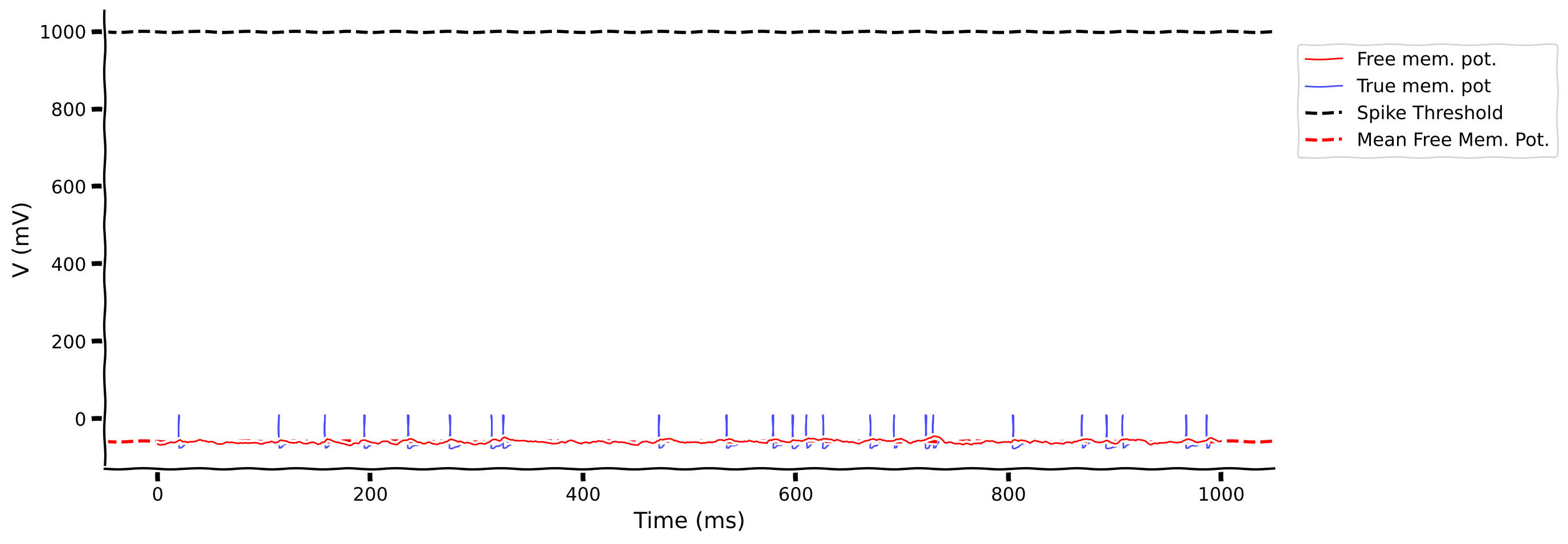
興奮性および抑制性入力の両方に対して、レート10 HzのPoisson_generatorで生成されたシナプス前スパイク列を用いてコンダクタンスベースのLIFニューロンをシミュレーションしましょう。ここでは、80本の興奮性シナプス前スパイク列と20本の抑制性スパイク列を選びます。

以前に、 $CV_{\rm ISI}$ が出力スパイクパターンの不規則性を記述できることを学びました。ここでは新たに、**自由膜電位（FMP）**というニューロン膜の指標を導入します。FMPはスパイク閾値を取り除いたときの膜電位です。

これは完全に人工的なものですが、この量を計算することで入力の強さを把握できます。特にFMPの平均と標準偏差（std.）に注目します。演習では、FMPとスパイク閾値付きの膜電位を可視化できます。

# Get default parameters
pars = default_pars(T=1000.)

# Add parameters
pars['gE_bar'] = 2.4    # [nS]
pars['VE'] = 0.         # [mV] excitatory reversal potential
pars['tau_syn_E'] = 2.  # [ms]
pars['gI_bar'] = 2.4    # [nS]
pars['VI'] = -80.       # [mV] inhibitory reversal potential
pars['tau_syn_I'] = 5.  # [ms]

# Generate presynaptic spike trains
pre_spike_train_ex = Poisson_generator(pars, rate=10, n=80)
pre_spike_train_in = Poisson_generator(pars, rate=10, n=20)

# Simulate conductance-based LIF model
v, rec_spikes, gE, gI = run_LIF_cond(pars, 0, pre_spike_train_ex,
                                     pre_spike_train_in)

# Show spikes more clearly by setting voltage high
dt, range_t = pars['dt'], pars['range_t']
if rec_spikes.size:
  sp_num = (rec_spikes / dt).astype(int) - 1
  v[sp_num] = 10   # draw nicer spikes

####################################################################
## TODO for students: measure the free membrane potential
# In order to measure the free membrane potential, first,
# you should prevent the firing of the LIF neuron
# How to prevent a LIF neuron from firing? Increase the threshold pars['V_th'].
raise NotImplementedError("Student exercise: change threshold and calculate FMP")
####################################################################

# Change the threshold
pars['V_th'] = ...

# Calculate FMP
v_fmp, _, _, _ = run_LIF_cond(pars, ..., ..., ...)

my_illus_LIFSYN(pars, v_fmp, v)

解答を見る$

出力例:

# @title Submit your feedback
content_review(f"{feedback_prefix}_Measure_the_mean_free_membrane_potential_Exercise")

インタラクティブデモ1.2: 異なる興奮性/抑制性入力によるコンダクタンスベースLIFエクスプローラー

以下では、興奮性と抑制性入力の比率を変化させることで、発火率とスパイク時間の規則性（出力テキスト参照）がどのように変わるかを調べられます。

興奮性および抑制性入力の両方を変えるために、それらの発火率を変化させます。ただし、必要に応じてこれらの接続の強さや数を変えてもかまいません。

自由膜電位の平均（赤点線）とスパイク閾値（黒点線）との位置関係に特に注目してください。

FMPの平均とスパイク時間の不規則性（ $CV_{\rm ISI}$ ）の間に関係はありますか？FMPの平均がスパイク閾値を超えた場合と下回った場合で何が起こりますか？

# @markdown Make sure you execute this cell to enable the widget!

my_layout.width = '450px'
@widgets.interact(
    inh_rate=widgets.FloatSlider(20., min=10., max=60., step=5.,
                                 layout=my_layout),
    exc_rate=widgets.FloatSlider(10., min=2., max=20., step=2.,
                                 layout=my_layout)
)


def EI_isi_regularity(exc_rate, inh_rate):

  pars = default_pars(T=1000.)
  # Add parameters
  pars['gE_bar'] = 3.     # [nS]
  pars['VE'] = 0.         # [mV] excitatory reversal potential
  pars['tau_syn_E'] = 2.  # [ms]
  pars['gI_bar'] = 3.     # [nS]
  pars['VI'] = -80.       # [mV] inhibitory reversal potential
  pars['tau_syn_I'] = 5.  # [ms]

  pre_spike_train_ex = Poisson_generator(pars, rate=exc_rate, n=80)
  pre_spike_train_in = Poisson_generator(pars, rate=inh_rate, n=20)  # 4:1

  # Lets first simulate a neuron with identical input but with no spike
  # threshold by setting the threshold to a very high value
  # so that we can look at the free membrane potential
  pars['V_th'] = 1e3
  v_fmp, rec_spikes, gE, gI = run_LIF_cond(pars, 0, pre_spike_train_ex,
                                           pre_spike_train_in)

  # Now simulate a LIP with a regular spike threshold
  pars['V_th'] = -55.
  v, rec_spikes, gE, gI = run_LIF_cond(pars, 0, pre_spike_train_ex,
                                       pre_spike_train_in)
  dt, range_t = pars['dt'], pars['range_t']
  if rec_spikes.size:
      sp_num = (rec_spikes / dt).astype(int) - 1
      v[sp_num] = 10  # draw nicer spikes

  spike_rate = 1e3 * len(rec_spikes) / pars['T']

  cv_isi = 0.
  if len(rec_spikes) > 3:
    isi = np.diff(rec_spikes)
    cv_isi = np.std(isi) / np.mean(isi)

  print('\n')
  plt.figure(figsize=(15, 10))
  plt.subplot(211)
  plt.text(500, -35, f'Spike rate = {spike_rate:.3f} (sp/s), Mean of Free Mem Pot = {np.mean(v_fmp):.3f}',
           fontsize=16, fontweight='bold', horizontalalignment='center',
           verticalalignment='bottom')
  plt.text(500, -38.5, f'CV ISI = {cv_isi:.3f}, STD of Free Mem Pot = {np.std(v_fmp):.3f}',
           fontsize=16, fontweight='bold', horizontalalignment='center',
           verticalalignment='bottom')

  plt.plot(pars['range_t'], v_fmp, 'r', lw=1.,
           label='Free mem. pot.', zorder=2)
  plt.plot(pars['range_t'], v, 'b', lw=1.,
           label='mem. pot with spk thr', zorder=1, alpha=0.7)
  plt.axhline(pars['V_th'], 0, 1, color='k', lw=1., ls='--',
              label='Spike Threshold', zorder=1)
  plt.axhline(np.mean(v_fmp),0, 1, color='r', lw=1., ls='--',
              label='Mean Free Mem. Pot.', zorder=1)
  plt.ylim(-76, -39)
  plt.xlabel('Time (ms)')
  plt.ylabel('V (mV)')
  plt.legend(loc=[1.02, 0.68])

  plt.subplot(223)
  plt.plot(pars['range_t'][::3], gE[::3], 'r', lw=1)
  plt.xlabel('Time (ms)')
  plt.ylabel(r'$g_E$ (nS)')

  plt.subplot(224)
  plt.plot(pars['range_t'][::3], gI[::3], 'b', lw=1)
  plt.xlabel('Time (ms)')
  plt.ylabel(r'$g_I$ (nS)')

  plt.tight_layout()
  plt.show()

解答を見る$

# @title Submit your feedback
content_review(f"{feedback_prefix}_LIF_Explorer_Interactive_Demo_and_Discussion")

考えてみよう！1.2: 興奮性と抑制性のバランス

スパイクパターンの変動性をどれくらい増やせますか？ニューロンがポアソン型スパイクで応答する条件は何でしょうか？（ポアソン型スパイクを注入していることに注意してください。答えは興奮性と抑制性入力スパイクレートの比率に関して考えてください。）
興奮性と抑制性のバランスに関連して：興奮性と抑制性のバランスの定義の一つは、興奮性と抑制性の入力レートが増加しても自由膜電位の平均が一定に保たれることです。ニューロンをバランス状態に保ちながら興奮性と抑制性のレートを変化させると、ニューロンの発火率はどうなると思いますか？詳細はKuhn, Aertsen, and Rotter (2004)を参照してください。

解答を見る$

# @title Submit your feedback
content_review(f"{feedback_prefix}_Excitatory_Inhibitory_balance_Discussion")

セクション2: 短期シナプス可塑性

チュートリアル開始からここまでの推定時間：45分

前述の通り、シナプスは固定重みでモデル化しました。ここからは、入力条件によって重みが変化するシナプスを探ります。

短期可塑性（STP）は、シナプス効力がシナプス前活動の履歴を反映して時間とともに変化する現象です。STPには、シナプス効力に逆の効果を持つ2種類が実験的に観察されています。これらは短期抑制（STD）と短期促進（STF）として知られています。

STPの数学モデル（詳細はこちら $）は、伝達に利用可能な限られたシナプス資源プール（$ R$）の概念に基づいています。例えば、シナプス前終末のシナプス小胞の総量などです。シナプス前資源の量はスパイクの最近の履歴に応じて動的に変化します。

シナプス前スパイクの後、(i) 利用可能プールのうち利用される割合 $u$ （放出確率）がスパイク誘発性カルシウム流入により増加し、(ii) $u$ が消費されてシナプス後コンダクタンスが増加します。スパイク間では、 $u$ は時定数 $\tau_f$ でゼロに減衰し、 $R$ は時定数 $\tau_d$ で1に回復します。まとめると、興奮性（添字 $E$ ）STPの動態は以下の通りです：

\begin{eqnarray}
&& $\frac{du_E}{dt}$ &=& - $\frac{u_E}{\tau_f} + U_0(1-u_E^-)\delta(t-t_{\rm sp})$ \[.5mm]
&& $\frac{dR_E}{dt}$ &=& $\frac{1-R_E}{\tau_d} - u_E^+ R_E^- \delta(t-t_{\rm sp}) \qquad (6)$ \[.5mm]
&& $\frac{dg_E(t)}{dt}$ &=& - $\frac{g_E}{\tau_E} + \bar{g}_E u_E^+ R_E^- \delta(t-t_{\rm sp}) \end{eqnarray}$

ここで、 $U_0$ はスパイクによって $u$ が増加する量を決める定数です。 $u_E^-$ と $R_E^-$ はスパイク直前の値、 $u_E^+$ はスパイク直後の値を示します。 $\bar{g}_E$ は最大興奮性コンダクタンスで、 $g_E(t)$ はすべてのスパイク時刻 $k$ に対して計算され、時定数 $\tau_{E}$ で減衰します。同様に、抑制性STPの動態は添字 $E$ を $I$ に置き換えて得られます。

$u$ と $R$ の動態の相互作用により、 $uR$ の総効果が抑制または促進のどちらに支配されるかが決まります。 $\tau_d \gg \tau_f$ かつ大きな $U_0$ のパラメータ領域では、初期スパイクで $R$ が大きく減少し回復に時間がかかるため、シナプスはSTD優勢です。 $\tau_d \ll \tau_f$ かつ小さな $U_0$ の領域では、スパイクによりシナプス効力が徐々に増加し、シナプスはSTF優勢となります。この現象論的モデルは、多くの皮質領域で観察される抑制および促進シナプスの動態をうまく再現します。

以下に、上記の方程式をオイラー法（昨日学んだ方法）で積分するヘルパー関数dynamic_synを提供します。

# @markdown Execute this cell to get helper function `dynamic_syn`

def dynamic_syn(g_bar, tau_syn, U0, tau_d, tau_f, pre_spike_train, dt):
  """
  Short-term synaptic plasticity

  Args:
    g_bar           : synaptic conductance strength
    tau_syn         : synaptic time constant [ms]
    U0              : synaptic release probability at rest
    tau_d           : synaptic depression time constant of x [ms]
    tau_f           : synaptic facilitation time constantr of u [ms]
    pre_spike_train : total spike train (number) input
                      from presynaptic neuron
    dt              : time step [ms]

  Returns:
    u               : usage of releasable neurotransmitter
    R               : fraction of synaptic neurotransmitter resources available
    g               : postsynaptic conductance

  """

  Lt = len(pre_spike_train)
  # Initialize
  u = np.zeros(Lt)
  R = np.zeros(Lt)
  R[0] = 1.
  g = np.zeros(Lt)

  # simulation
  for it in range(Lt - 1):
    # Compute du
    du = -(dt / tau_f) * u[it] + U0 * (1.0 - u[it]) * pre_spike_train[it + 1]
    u[it + 1] = u[it] + du
    # Compute dR
    dR = (dt / tau_d) * (1.0 - R[it]) - u[it + 1] * R[it] * pre_spike_train[it + 1]
    R[it + 1] = R[it] + dR
    # Compute dg
    dg = -(dt / tau_syn) * g[it] + g_bar * R[it] * u[it + 1] * pre_spike_train[it + 1]
    g[it + 1] = g[it] + dg

  return u, R, g

help(dynamic_syn)

セクション2.1: 短期シナプス抑制（STD）

インタラクティブデモ 2.1: 入力レートによるSTDエクスプローラー

以下は、短期シナプス抑圧（STD）が、入力側のスパイク列の発火率によってどのように変化するか、またシナプスコンダクタンスの振幅 $g$ が各スパイクごとにどのように変化し、定常状態に達するかを示すインタラクティブデモです。

発火率はシナプス効力にどのような影響を与えるでしょうか？
ニューロンが規則的に発火するのではなく、ポアソン的に発火する場合はどうでしょうか？

注意： Poisson=True はポアソン型、Poisson=False は規則的な入力スパイクを意味します。対応するチェックボックスをオン・オフして確認できます。

# @markdown Make sure you execute this cell to enable the widget!

my_layout.width = '450px'
@widgets.interact(
    rate=widgets.FloatSlider(10., min=10., max=100., step=5., layout=my_layout),
    Poisson=widgets.Checkbox(value=False, layout=my_layout)
)

def my_STD_diff_rate(rate, Poisson):
      _ = my_illus_STD(Poisson=Poisson, rate=rate)

解答を見る$

# @title Submit your feedback
content_review(f"{feedback_prefix}_STD_Explorer_with_input_rate_Interactive_Demo_and_Discussion")

かつて、実験者に大脳皮質の興奮性ニューロン間の接続によって生じるPSP振幅の実験値について尋ねたことがあります。彼女は「どの周波数でですか？」と聞き返しました。私は戸惑いましたが、スパイク履歴、つまり入力ニューロンの発火率に依存してPSP振幅が変わることを知れば、彼女の質問の意味がわかるでしょう。

ここでは、シナプスコンダクタンスの1回目と10回目のスパイクに対応する比率が、入力側の発火率の関数としてどのように変化するかを調べます（実験者はしばしば1回目と2回目のPSPの比を取ります）。

計算効率のために、入力スパイクは規則的であると仮定します。この仮定により、複数回の試行を行う必要がなくなります。

# @markdown STD conductance ratio with different input rate
# Regular firing rate
input_rate = np.arange(5., 40.1, 5.)
g_1 = np.zeros(len(input_rate))  # record the the PSP at 1st spike
g_2 = np.zeros(len(input_rate))  # record the the PSP at 10th spike

for ii in range(len(input_rate)):
   g_1[ii], g_2[ii] = my_illus_STD(Poisson=False, rate=input_rate[ii],
                                   plot_out=False, U0=0.5, tau_d=100., tau_f=50)

plt.figure(figsize=(11, 4.5))

plt.subplot(121)
plt.plot(input_rate, g_1, 'm-o', label='1st Spike')
plt.plot(input_rate, g_2, 'c-o', label='10th Spike')
plt.xlabel('Rate [Hz]')
plt.ylabel('Conductance [nS]')
plt.legend()

plt.subplot(122)
plt.plot(input_rate, g_2 / g_1, 'b-o')
plt.xlabel('Rate [Hz]')
plt.ylabel(r'Conductance ratio $g_{10}/g_{1}$')\

plt.tight_layout()
plt.show()

入力レートを上げると、1回目と10回目のスパイクの比率は増加します。これは10回目のスパイクのコンダクタンスが小さくなるためです。これは、同じ量の電流を使ってもニューロンへの効果が小さくなるという、シナプス抑圧の明確な証拠です。

セクション 2.2: 短期シナプス促進（STF）

インタラクティブデモ 2.2: 入力レートによるSTFエクスプローラー

以下は短期促進の例のイラストです。シナプス変数 $U_0$ 、tau_d、および tau_f の変化に注目してください。

STDの場合、U0=0.5, tau_d=100., tau_f=50.
STPの場合、U0=0.2, tau_d=100., tau_f=750.

入力レートを変化させるとシナプスコンダクタンスはどのように変わりますか？規則的な入力とポアソン型の入力の場合で何を観察しますか？

# @markdown Make sure you execute this cell to enable the widget!

my_layout.width = '450px'
@widgets.interact(
    rate=widgets.FloatSlider(10., min=4., max=40., step=2., layout=my_layout),
    Poisson=widgets.Checkbox(value=False, layout=my_layout)
)


def my_STD_diff_rate(rate, Poisson):
  _ = my_illus_STD(Poisson=Poisson, rate=rate,
                   U0=0.2, tau_d=100., tau_f=750.)

考えてみよう！ 2.2: 短期シナプス促進と抑圧の比較

ここでは、 $1^{st}$ と $10^{th}$ スパイクに対応するシナプスコンダクタンスの比率が、入力側の発火率の関数としてどのように変化するかを調べます。

なぜ、STFを持つシナプスでは1回目と10回目のスパイクコンダクタンスの比率が単調増加しないのに対し、STDを持つシナプスでは単調減少するのでしょうか？

# @markdown STF conductance ratio with different input rates
# Regular firing rate
input_rate = np.arange(2., 40.1, 2.)
g_1 = np.zeros(len(input_rate))  # record the the PSP at 1st spike
g_2 = np.zeros(len(input_rate))  # record the the PSP at 10th spike

for ii in range(len(input_rate)):
   g_1[ii], g_2[ii] = my_illus_STD(Poisson=False, rate=input_rate[ii],
                                   plot_out=False,
                                   U0=0.2, tau_d=100., tau_f=750.)

plt.figure(figsize=(11, 4.5))

plt.subplot(121)
plt.plot(input_rate, g_1, 'm-o', label='1st Spike')
plt.plot(input_rate, g_2, 'c-o', label='10th Spike')
plt.xlabel('Rate [Hz]')
plt.ylabel('Conductance [nS]')
plt.legend()

plt.subplot(122)
plt.plot(input_rate, g_2 / g_1, 'b-o',)
plt.xlabel('Rate [Hz]')
plt.ylabel(r'Conductance ratio $g_{10}/g_{1}$')

plt.tight_layout()
plt.show()

解答を見る$

# @title Submit your feedback
content_review(f"{feedback_prefix}_STF_Explorer_with_input_rate_Interactive_Demo_and_Discussion")

まとめ

チュートリアルの推定所要時間：1時間10分

おめでとうございます！本日の最後のチュートリアルを終えました。ここでは、コンダクタンスベースのシナプスのモデル化方法と、シナプス重みに短期動的変化を組み込む方法を学びました。

扱った内容は以下の通りです：

静的シナプスと、興奮性および抑制性がニューロン出力に与える影響
平均駆動または変動駆動の状態
シナプスの短期動態（促進と抑圧の両方）

最後に、これらのツールを組み合わせて、入力側の発火履歴の変化がシナプス重みにどのように影響するかを調べました！

生物学的シナプスの理解を深めるために、自分で試してみると面白いことがたくさんあります。いくつかは以下のオプションボックスに記載していますので、時間があればぜひ挑戦してください。

時間があれば、以下のボーナスセクションでSTPを持つコンダクタンスベースのLIFモデルも見てみてください。また、スパイクタイミング依存性シナプス可塑性に関するボーナスチュートリアルも用意されています！

ボーナス

ボーナスセクション1：STPを考慮した導電率ベースのLIFモデル

これまで、シナプス前の発火率がシナプス前資源の利用可能性にどのように影響し、それによってシナプス導電率がどう変わるかだけを見てきました。シナプス導電率が変化している間、シナプス後ニューロンの出力も変わることは容易に想像できます。

それでは、STPをLIFニューロンに入力するシナプスに適用して、何が起こるか見てみましょう。

# @markdown Execute for helper function for conductance-based LIF neuron with STP-synapses

def run_LIF_cond_STP(pars, I_inj, pre_spike_train_ex, pre_spike_train_in):
  """
  conductance-based LIF dynamics

  Args:
    pars               : parameter dictionary
    I_inj              : injected current [pA]
                         The injected current here can be a value or an array
    pre_spike_train_ex : spike train input from presynaptic excitatory neuron (binary)
    pre_spike_train_in : spike train input from presynaptic inhibitory neuron (binary)

  Returns:
    rec_spikes : spike times
    rec_v      : mebrane potential
    gE         : postsynaptic excitatory conductance
    gI         : postsynaptic inhibitory conductance

  """

  # Retrieve parameters
  V_th, V_reset = pars['V_th'], pars['V_reset']
  tau_m, g_L = pars['tau_m'], pars['g_L']
  V_init, V_L = pars['V_init'], pars['E_L']
  gE_bar, gI_bar = pars['gE_bar'], pars['gI_bar']
  U0E, tau_dE, tau_fE = pars['U0_E'], pars['tau_d_E'], pars['tau_f_E']
  U0I, tau_dI, tau_fI = pars['U0_I'], pars['tau_d_I'], pars['tau_f_I']
  VE, VI = pars['VE'], pars['VI']
  tau_syn_E, tau_syn_I = pars['tau_syn_E'], pars['tau_syn_I']
  tref = pars['tref']

  dt, range_t = pars['dt'], pars['range_t']
  Lt = range_t.size

  nE = pre_spike_train_ex.shape[0]
  nI = pre_spike_train_in.shape[0]

  # compute conductance Excitatory synapses
  uE = np.zeros((nE, Lt))
  RE = np.zeros((nE, Lt))
  gE = np.zeros((nE, Lt))
  for ie in range(nE):
    u, R, g = dynamic_syn(gE_bar, tau_syn_E, U0E, tau_dE, tau_fE,
                          pre_spike_train_ex[ie, :], dt)

    uE[ie, :], RE[ie, :], gE[ie, :] = u, R, g

  gE_total = gE.sum(axis=0)

  # compute conductance Inhibitory synapses
  uI = np.zeros((nI, Lt))
  RI = np.zeros((nI, Lt))
  gI = np.zeros((nI, Lt))
  for ii in range(nI):
    u, R, g = dynamic_syn(gI_bar, tau_syn_I, U0I, tau_dI, tau_fI,
                          pre_spike_train_in[ii, :], dt)

    uI[ii, :], RI[ii, :], gI[ii, :] = u, R, g

  gI_total = gI.sum(axis=0)

  # Initialize
  v = np.zeros(Lt)
  v[0] = V_init
  Iinj = I_inj * np.ones(Lt)  # ensure I has length Lt

  # simulation
  rec_spikes = []  # recording spike times
  tr = 0.
  for it in range(Lt - 1):
    if tr > 0:
      v[it] = V_reset
      tr = tr - 1
    elif v[it] >= V_th:  # reset voltage and record spike event
      rec_spikes.append(it)
      v[it] = V_reset
      tr = tref / dt

    # calculate the increment of the membrane potential
    dv = (dt / tau_m) * (-(v[it] - V_L) \
                         - (gE_total[it + 1] / g_L) * (v[it] - VE) \
                         - (gI_total[it + 1] / g_L) * (v[it] - VI) + Iinj[it] / g_L)

    # update membrane potential
    v[it+1] = v[it] + dv

  rec_spikes = np.array(rec_spikes) * dt

  return v, rec_spikes, uE, RE, gE, RI, RI, gI


help(run_LIF_cond_STP)

ボーナスインタラクティブデモ：STP付きLIFエクスプローラー

ここでは、興奮性および抑制性シナプスの両方が短期抑制を示すと仮定しています。シナプスの性質を変更して、スパイクパターンの変動性がどのように変わるかを調べてみてください。
このデモでは、tau_d = 500*tau_ratio (ms) および tau_f = 300*tau_ratio (ms) としています。

このニューロンの出力を、前のチュートリアルでシナプスが静的と仮定した場合に観察したものと比較してください。

注：各ケースの実行には少し時間がかかります

# @markdown Make sure you execute this cell to enable the widget!
my_layout.width = '450px'
@widgets.interact(
    tau_ratio=widgets.FloatSlider(0.5, min=.2, max=1.,
                                  step=.2, layout=my_layout),
)


def LIF_STP(tau_ratio):
  pars = default_pars(T=1000)
  pars['gE_bar'] = 1.2 * 4  # [nS]
  pars['VE'] = 0.           # [mV]
  pars['tau_syn_E'] = 5.    # [ms]
  pars['gI_bar'] = 1.6 * 4  # [nS]
  pars['VI'] = -80.         # [ms]
  pars['tau_syn_I'] = 10.   # [ms]

  # here we assume that both Exc and Inh synapses have synaptic depression
  pars['U0_E'] = 0.45
  pars['tau_d_E'] = 500. * tau_ratio  # [ms]
  pars['tau_f_E'] = 300. * tau_ratio  # [ms]

  pars['U0_I'] = 0.45
  pars['tau_d_I'] = 500. * tau_ratio  # [ms]
  pars['tau_f_I'] = 300. * tau_ratio  # [ms]

  pre_spike_train_ex = Poisson_generator(pars, rate=15, n=80)
  pre_spike_train_in = Poisson_generator(pars, rate=15, n=20)  # 4:1

  v, rec_spikes, uE, RE, gE, uI, RI, gI = run_LIF_cond_STP(pars, 0,
                                                           pre_spike_train_ex,
                                                           pre_spike_train_in)

  t_plot_range = pars['range_t'] > 200

  plt.figure(figsize=(11, 7))
  plt.subplot(211)
  plot_volt_trace(pars, v, rec_spikes, show=False)

  plt.subplot(223)
  plt.plot(pars['range_t'][t_plot_range], gE.sum(axis=0)[t_plot_range], 'r')
  plt.xlabel('Time (ms)')
  plt.ylabel(r'$g_E$ (nS)')

  plt.subplot(224)
  plt.plot(pars['range_t'][t_plot_range], gI.sum(axis=0)[t_plot_range], 'b')
  plt.xlabel('Time (ms)')
  plt.ylabel(r'$g_I$ (nS)')

  plt.tight_layout()
  plt.show()

tau_ratio を変化させると、tau_f と tau_d が増加します。つまり、tau_ratio を増やすことでシナプス抑制が強くなります。この効果は興奮性および抑制性の導電率の両方に同様に現れます。
これは、300～400ms以降にニューロンの発火率が明確に低下することで確認できます。

初めのうちはあまり変化が見られません。なぜならシナプス抑制が目に見えるようになるまでに時間がかかるためです。

興味深いことに、興奮性および抑制性の導電率が共に抑制されているにもかかわらず、出力発火率は依然として低下しています。

これには2つの説明があります：

興奮性は開始時の値から抑制性よりも大きく抑制されている。
シナプス導電率が抑制されたため、膜電位の変動幅が小さくなった。

どちらがより可能性が高い理由でしょうか？

# @title Submit your feedback
content_review(f"{feedback_prefix}_LIF_with_STP_Bonus_Interactive_Demo")

シナプスにSTPがある場合、ニューロンはより高い不規則性を示すでしょうか？

STP付きLIFニューロンをシミュレーションした後、異なる tau_ratio で $CV_{\rm ISI}$ を計算してみてください（ヒント：run_LIF_cond_STP が不規則性の理解に役立ちます）。

シナプスの短期動態の機能的意義

上記で見たように、発火率が定常的であれば、シナプス導電率はすぐに定常点に達します。一方、発火率が一時的に変化すると、シナプス導電率も変動します――たとえその変化が単一のスパイク間隔の長さであっても。入力スパイクが規則的かつ周期的であれば、単一ニューロンでもこうした小さな変化を観察できます。入力スパイクがポアソン分布的であれば、複数のニューロンで平均を取る必要があるかもしれません。

シナプスの短期動態を利用して実装できる他の機能を考え、それらを実装してみてください。