チュートリアル 2: 入力相関の効果

第2週目, 4日目: 生物学的ニューロンモデル

Neuromatch Academyによる

コンテンツ作成者: Qinglong Gu, Songtin Li, John Murray, Richard Naud, Arvind Kumar

コンテンツレビュアー: Maryam Vaziri-Pashkam, Ella Batty, Lorenzo Fontolan, Richard Gao, Matthew Krause, Spiros Chavlis, Michael Waskom

ポストプロダクションチーム: Gagana B, Spiros Chavlis

チュートリアルの目的

推定所要時間: 50分

このチュートリアルでは、リーキー積分発火（LIF）ニューロンモデル（チュートリアル1参照）を用いて、入力の相関が出力特性にどのように変換されるか（相関の伝達）を調べます。具体的には、以下のコードを数行書きます:

相関のあるガウス白色雑音（GWN）を2つのニューロンに注入する
2つのニューロンのスパイク活動間の相関を測定する
入力の統計量（平均と標準偏差）によって相関の伝達がどのように変わるかを調べる

# @title Tutorial slides
# @markdown These are the slides for the videos in all tutorials today
from IPython.display import IFrame
link_id = "8djsm"
print(f"If you want to download the slides: https://osf.io/download/{link_id}/")
IFrame(src=f"https://mfr.ca-1.osf.io/render?url=https://osf.io/{link_id}/?direct%26mode=render%26action=download%26mode=render", width=854, height=480)

セットアップ

# @title Install and import feedback gadget


from vibecheck import DatatopsContentReviewContainer
def content_review(notebook_section: str):
    return DatatopsContentReviewContainer(
        "",  # No text prompt
        notebook_section,
        {
            "url": "https://pmyvdlilci.execute-api.us-east-1.amazonaws.com/klab",
            "name": "neuromatch_cn",
            "user_key": "y1x3mpx5",
        },
    ).render()


feedback_prefix = "W2D3_T2"

# Imports
import matplotlib.pyplot as plt
import numpy as np
import time

# @title Figure Settings
import logging
logging.getLogger('matplotlib.font_manager').disabled = True

import ipywidgets as widgets  # interactive display
%config InlineBackend.figure_format = 'retina'
# use NMA plot style
plt.style.use("https://raw.githubusercontent.com/NeuromatchAcademy/course-content/main/nma.mplstyle")
my_layout = widgets.Layout()

# @title Plotting Functions

def example_plot_myCC():
  pars = default_pars(T=50000, dt=.1)

  c = np.arange(10) * 0.1
  r12 = np.zeros(10)
  for i in range(10):
    I1gL, I2gL = correlate_input(pars, mu=20.0, sig=7.5, c=c[i])
    r12[i] = my_CC(I1gL, I2gL)

  plt.figure()
  plt.plot(c, r12, 'bo', alpha=0.7, label='Simulation', zorder=2)
  plt.plot([-0.05, 0.95], [-0.05, 0.95], 'k--', label='y=x',
           dashes=(2, 2), zorder=1)
  plt.xlabel('True CC')
  plt.ylabel('Sample CC')
  plt.legend(loc='best')
  plt.show()


def my_raster_Poisson(range_t, spike_train, n):
  """
  Ffunction generates and plots the raster of the Poisson spike train

  Args:
    range_t     : time sequence
    spike_train : binary spike trains, with shape (N, Lt)
    n           : number of Poisson trains plot

  Returns:
    Raster plot of the spike train
  """

  # find the number of all the spike trains
  N = spike_train.shape[0]

  # n should smaller than N:
  if n > N:
    print('The number n exceeds the size of spike trains')
    print('The number n is set to be the size of spike trains')
    n = N

  # plot rater
  plt.figure()
  i = 0
  while i < n:
    if spike_train[i, :].sum() > 0.:
      t_sp = range_t[spike_train[i, :] > 0.5]  # spike times
      plt.plot(t_sp, i * np.ones(len(t_sp)), 'k|', ms=10, markeredgewidth=2)
    i += 1
  plt.xlim([range_t[0], range_t[-1]])
  plt.ylim([-0.5, n + 0.5])
  plt.xlabel('Time (ms)', fontsize=12)
  plt.ylabel('Neuron ID', fontsize=12)
  plt.show()

def plot_c_r_LIF(c, r, mycolor, mylabel):
  z = np.polyfit(c, r, deg=1)
  c_range = np.array([c.min() - 0.05, c.max() + 0.05])
  plt.plot(c, r, 'o', color=mycolor, alpha=0.7, label=mylabel, zorder=2)
  plt.plot(c_range, z[0] * c_range + z[1], color=mycolor, zorder=1)

# @title Helper Functions
def default_pars(**kwargs):
  pars = {}

  ### typical neuron parameters###
  pars['V_th'] = -55.     # spike threshold [mV]
  pars['V_reset'] = -75.  # reset potential [mV]
  pars['tau_m'] = 10.     # membrane time constant [ms]
  pars['g_L'] = 10.       # leak conductance [nS]
  pars['V_init'] = -75.   # initial potential [mV]
  pars['V_L'] = -75.      # leak reversal potential [mV]
  pars['tref'] = 2.       # refractory time (ms)

  ### simulation parameters ###
  pars['T'] = 400. # Total duration of simulation [ms]
  pars['dt'] = .1  # Simulation time step [ms]

  ### external parameters if any ###
  for k in kwargs:
    pars[k] = kwargs[k]

  pars['range_t'] = np.arange(0, pars['T'], pars['dt'])  # Vector of discretized
                                                         # time points [ms]
  return pars


def run_LIF(pars, Iinj):
  """
  Simulate the LIF dynamics with external input current

  Args:
    pars       : parameter dictionary
    Iinj       : input current [pA]. The injected current here can be a value or an array

  Returns:
    rec_spikes : spike times
    rec_v      : mebrane potential
  """

  # Set parameters
  V_th, V_reset = pars['V_th'], pars['V_reset']
  tau_m, g_L = pars['tau_m'], pars['g_L']
  V_init, V_L = pars['V_init'], pars['V_L']
  dt, range_t = pars['dt'], pars['range_t']
  Lt = range_t.size
  tref = pars['tref']

  # Initialize voltage and current
  v = np.zeros(Lt)
  v[0] = V_init
  Iinj = Iinj * np.ones(Lt)
  tr = 0.

  # simulate the LIF dynamics
  rec_spikes = []   # record spike times
  for it in range(Lt - 1):
    if tr > 0:
      v[it] = V_reset
      tr = tr - 1
    elif v[it] >= V_th:  # reset voltage and record spike event
      rec_spikes.append(it)
      v[it] = V_reset
      tr = tref / dt

    # calculate the increment of the membrane potential
    dv = (-(v[it] - V_L) + Iinj[it] / g_L) * (dt / tau_m)

    # update the membrane potential
    v[it + 1] = v[it] + dv

  rec_spikes = np.array(rec_spikes) * dt

  return v, rec_spikes


def my_GWN(pars, sig, myseed=False):
  """
  Function that calculates Gaussian white noise inputs

  Args:
    pars       : parameter dictionary
    mu         : noise baseline (mean)
    sig        : noise amplitute (standard deviation)
    myseed     : random seed. int or boolean
                 the same seed will give the same random number sequence

  Returns:
    I          : Gaussian white noise input
  """

  # Retrieve simulation parameters
  dt, range_t = pars['dt'], pars['range_t']
  Lt = range_t.size

  # Set random seed. You can fix the seed of the random number generator so
  # that the results are reliable however, when you want to generate multiple
  # realization make sure that you change the seed for each new realization
  if myseed:
      np.random.seed(seed=myseed)
  else:
      np.random.seed()

  # generate GWN
  # we divide here by 1000 to convert units to sec.
  I_GWN = sig * np.random.randn(Lt) * np.sqrt(pars['tau_m'] / dt)

  return I_GWN


def LIF_output_cc(pars, mu, sig, c, bin_size, n_trials=20):
  """ Simulates two LIF neurons with correlated input and computes output correlation

  Args:
  pars       : parameter dictionary
  mu         : noise baseline (mean)
  sig        : noise amplitute (standard deviation)
  c          : correlation coefficient ~[0, 1]
  bin_size   : bin size used for time series
  n_trials   : total simulation trials

  Returns:
  r          : output corr. coe.
  sp_rate    : spike rate
  sp1        : spike times of neuron 1 in the last trial
  sp2        : spike times of neuron 2 in the last trial
  """

  r12 = np.zeros(n_trials)
  sp_rate = np.zeros(n_trials)
  for i_trial in range(n_trials):
    I1gL, I2gL = correlate_input(pars, mu, sig, c)
    _, sp1 = run_LIF(pars, pars['g_L'] * I1gL)
    _, sp2 = run_LIF(pars, pars['g_L'] * I2gL)

    my_bin = np.arange(0, pars['T'], bin_size)

    sp1_count, _ = np.histogram(sp1, bins=my_bin)
    sp2_count, _ = np.histogram(sp2, bins=my_bin)

    r12[i_trial] = my_CC(sp1_count[::20], sp2_count[::20])
    sp_rate[i_trial] = len(sp1) / pars['T'] * 1000.

  return r12.mean(), sp_rate.mean(), sp1, sp2

ヘルパー関数には以下が含まれます:

パラメータ辞書: チュートリアル1の $default_pars(**kwargs)$
LIFシミュレータ: チュートリアル1の run_LIF
ガウス白色雑音生成器: チュートリアル1の my_GWN(pars, sig, myseed=False)
ポアソン型スパイク列生成器: Poisson_generator(pars, rate, n, myseed=False)
相関入力を持つ2つのLIFニューロンのシミュレータ: LIF_output_cc(pars, mu, sig, c, bin_size, n_trials=20)

セクション1: 相関（同期性）

ニューロン活動の相関または同期性は、脳活動の任意のリードアウトに対して記述できます。ここではニューロンのスパイク活動に注目します。

最も単純な形では、相関／同期性はニューロンの同時スパイクを指します。すなわち、2つのニューロンが同時にスパイクすると、それらは同期しているまたは相関していると言います。ニューロンは瞬間的な活動で同期することがあり、すなわちある確率で同時にスパイクします。しかし、あるニューロンの時刻 $t$ のスパイクが、遅延を伴って別のニューロンのスパイクと相関することもあります（時間遅延同期）。

同期的ニューロン活動の起源:

共通入力、すなわち2つのニューロンが同じ入力源から入力を受けている。共有入力の相関度合いは出力相関に比例する。
同じ入力源からのプーリング。ニューロンは同じ入力ニューロンを共有しないが、相関のあるニューロンから入力を受けている。
ニューロン同士が（単方向または双方向に）接続されている: これは時間遅延同期のみを生じる。ギャップジャンクションを介した接続もありうる。
ニューロンが類似のパラメータや初期条件を持つ。

同期性の意味

ニューロンが同時にスパイクすると、下流のニューロンにより強い影響を与えられます。脳のシナプスは、前後シナプス活動間の時間的相関（遅延）に敏感であり、これが機能的なニューロンネットワークの形成につながります。これは教師なし学習の基礎となります（これらの概念は今後のチュートリアルで学びます）。

同期性はシステムの次元削減を意味します。さらに、多くの場合、相関はニューロン活動のデコードを妨げることがあります。

# @title Video 1: Input & output correlations
from ipywidgets import widgets
from IPython.display import YouTubeVideo
from IPython.display import IFrame
from IPython.display import display


class PlayVideo(IFrame):
  def __init__(self, id, source, page=1, width=400, height=300, **kwargs):
    self.id = id
    if source == 'Bilibili':
      src = f'https://player.bilibili.com/player.html?bvid={id}&page={page}'
    elif source == 'Osf':
      src = f'https://mfr.ca-1.osf.io/render?url=https://osf.io/download/{id}/?direct%26mode=render'
    super(PlayVideo, self).__init__(src, width, height, **kwargs)


def display_videos(video_ids, W=400, H=300, fs=1):
  tab_contents = []
  for i, video_id in enumerate(video_ids):
    out = widgets.Output()
    with out:
      if video_ids[i][0] == 'Youtube':
        video = YouTubeVideo(id=video_ids[i][1], width=W,
                             height=H, fs=fs, rel=0)
        print(f'Video available at https://youtube.com/watch?v={video.id}')
      else:
        video = PlayVideo(id=video_ids[i][1], source=video_ids[i][0], width=W,
                          height=H, fs=fs, autoplay=False)
        if video_ids[i][0] == 'Bilibili':
          print(f'Video available at https://www.bilibili.com/video/{video.id}')
        elif video_ids[i][0] == 'Osf':
          print(f'Video available at https://osf.io/{video.id}')
      display(video)
    tab_contents.append(out)
  return tab_contents


video_ids = [('Youtube', 'nsAYFBcAkes'), ('Bilibili', 'BV1Bh411o7eV')]
tab_contents = display_videos(video_ids, W=854, H=480)
tabs = widgets.Tab()
tabs.children = tab_contents
for i in range(len(tab_contents)):
  tabs.set_title(i, video_ids[i][0])
display(tabs)

# @title Submit your feedback
content_review(f"{feedback_prefix}_Input_and_Output_correlations_Video")

相関の発生を調べる簡単なモデルは、2つのニューロンに共通入力を注入し、共通入力の割合に応じた出力相関を測定することです。

ここでは、相関入力を受けた2つの非接続LIFニューロンのスパイク列の相関係数を計算して、相関の伝達を調べます。

LIFニューロン $i$ $(i=1,2)$ への入力電流は:

\frac{I_i}{g_L} = \mu_i + \sigma_i (\sqrt{1-c}\xi_i + \sqrt{c}\xi_c) \quad (1)

ここで $\mu_i$ は電流の時間平均です。ガウス白色雑音 $\xi_i$ は各ニューロンで独立ですが、 $\xi_c$ は全ニューロンで共通です。変数 $c$ ( $0\le c\le1$ ) は共通入力と独立入力の割合を制御します。 $\sigma_i$ は総入力の分散を示します。

まず、相関入力を生成します。

# @markdown Execute this cell to get a function `correlate_input` for generating correlated GWN inputs
def correlate_input(pars, mu=20., sig=7.5, c=0.3):
  """
  Args:
    pars       : parameter dictionary
    mu         : noise baseline (mean)
    sig        : noise amplitute (standard deviation)
    c.         : correlation coefficient ~[0, 1]

  Returns:
    I1gL, I2gL : two correlated inputs with corr. coe. c
  """

  # generate Gaussian whute noise xi_1, xi_2, xi_c
  xi_1 = my_GWN(pars, sig)
  xi_2 = my_GWN(pars, sig)
  xi_c = my_GWN(pars, sig)

  # Generate two correlated inputs by Equation. (1)
  I1gL = mu + np.sqrt(1. - c) * xi_1 + np.sqrt(c) * xi_c
  I2gL = mu + np.sqrt(1. - c) * xi_2 + np.sqrt(c) * xi_c

  return I1gL, I2gL

help(correlate_input)

コーディング演習 1A: 相関の計算

2つの入力電流 $I_i$ と $I_j$ の_標本相関係数_は、 $I_i$ と $I_j$ の標本共分散を、 $I_i$ と $I_j$ の標本分散の平方根の積で割ったものとして定義されます。式で表すと:

\begin{align}
$r_{ij}$ &= $\frac{cov(I_i, I_j)}{\sqrt{var(I_i)} \sqrt{var(I_j)}}$ \
$cov(I_i,$ $I_j)$ &= $\sum_{k=1}^L (I_i^k -\bar{I_i})(I_j^k -\bar{I_j})$ \
$var(I_i)$ &= $\sum_{k=1}^L (I_i^k -\bar{I}_i)^2 \end{align}$

ここで $\bar{I_i}$ は標本平均、 $k$ は時間ビン、 $L$ は $I$ の長さを示します。つまり $I_i^k$ は時刻 $k\cdot dt$ の電流 $i$ です。

重要な注意: 上記の式は標本共分散と分散としては正確ではなく、 $L-1$ で割るべきですが、標本相関係数の式ではこの項が打ち消し合うため省略しています。

標本相関係数 は 標本ピアソン相関係数 とも呼ばれます。相関の計算と理解の多様な方法を解説した素晴らしい論文があります: Rodgers and Nicewander 1988。

この演習では、2つの時系列間の標本相関係数を計算する関数 my_CC を作成します。ここでは入力電流の文脈で紹介しましたが、標本相関係数は任意の2つの時系列の相関計算に使えます。後でビン化したスパイク列にも使います。

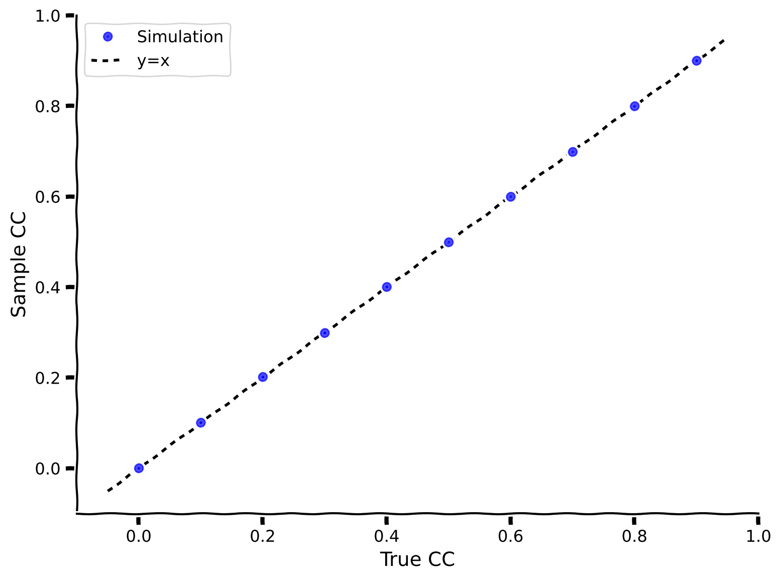
次に、ある相関を持つ電流を生成し（correlate_input を使用）、my_CC で相関係数を計算し、真の相関係数と標本相関係数をプロットして方法の正確さを確認します。

def my_CC(i, j):
  """
  Args:
    i, j  : two time series with the same length

  Returns:
    rij   : correlation coefficient
  """
  ########################################################################
  ## TODO for students: compute rxy, then remove the NotImplementedError #
  # Tip1: array([a1, a2, a3])*array([b1, b2, b3]) = array([a1*b1, a2*b2, a3*b3])
  # Tip2: np.sum(array([a1, a2, a3])) = a1+a2+a3
  # Tip3: square root, np.sqrt()
  # Fill out function and remove
  raise NotImplementedError("Student exercise: compute the sample correlation coefficient")
  ########################################################################

  # Calculate the covariance of i and j
  cov = ...

  # Calculate the variance of i
  var_i = ...

  # Calculate the variance of j
  var_j = ...

  # Calculate the correlation coefficient
  rij = ...

  return rij


example_plot_myCC()

解答を見る$

出力例:

# @title Submit your feedback
content_review(f"{feedback_prefix}_Compute_the_correlation_Exercise")

標本相関係数（my_CCで計算）が真の相関係数と一致しています！

次の演習ではポアソン分布を使ってスパイク列をモデル化します。ポアソン分布をこのように使うのは、統計学の前提条件の数学日で見たことを思い出してください。ポアソンスパイク列は以下の性質を持ちます:

スパイク数の平均と分散の比は1
スパイク間隔は指数分布
スパイク時刻は不規則、すなわち $CV_{ISI}=1$
隣接するスパイク間隔は独立

以下のセルでは、ヘルパー関数 Poisson_generator を提供し、それを使ってポアソンスパイク列を生成します。

# @markdown Execute this cell to get helper function `Poisson_generator`
def Poisson_generator(pars, rate, n, myseed=False):
  """
  Generates poisson trains

  Args:
    pars       : parameter dictionary
    rate       : noise amplitute [Hz]
    n          : number of Poisson trains
    myseed     : random seed. int or boolean

  Returns:
    pre_spike_train : spike train matrix, ith row represents whether
                      there is a spike in ith spike train over time
                      (1 if spike, 0 otherwise)
  """

  # Retrieve simulation parameters
  dt, range_t = pars['dt'], pars['range_t']
  Lt = range_t.size

  # set random seed
  if myseed:
      np.random.seed(seed=myseed)
  else:
      np.random.seed()

  # generate uniformly distributed random variables
  u_rand = np.random.rand(n, Lt)

  # generate Poisson train
  poisson_train = 1. * (u_rand < rate * (dt / 1000.))

  return poisson_train

help(Poisson_generator)

# @markdown Execute this cell to visualize Poisson spike train

pars = default_pars()
pre_spike_train = Poisson_generator(pars, rate=10, n=100, myseed=2020)
my_raster_Poisson(pars['range_t'], pre_spike_train, 100)

コーディング演習 1B: スパイク列間の相関を測定する

2つのニューロンのスパイク時刻を記録した後、どうやって相関係数を推定できますか？

これを求めるには、スパイク時刻をビン化して2つの時系列を得る必要があります。時系列の各データ点は対応する時間ビン内のスパイク数です。np.histogram() を使ってスパイク時刻をビン化できます。

以下のコードを完成させて、スパイク時刻をビン化し、2つのポアソンスパイク列の相関係数を計算してください。ここでの c は真の相関係数です。

# @markdown Execute this cell to get a function for generating correlated Poisson inputs (`generate_corr_Poisson`)


def generate_corr_Poisson(pars, poi_rate, c, myseed=False):
  """
  function to generate correlated Poisson type spike trains
  Args:
    pars       : parameter dictionary
    poi_rate   : rate of the Poisson train
    c.         : correlation coefficient ~[0, 1]

  Returns:
    sp1, sp2   : two correlated spike time trains with corr. coe. c
  """

  range_t = pars['range_t']

  mother_rate = poi_rate / c
  mother_spike_train = Poisson_generator(pars, rate=mother_rate,
                                         n=1, myseed=myseed)[0]
  sp_mother = range_t[mother_spike_train > 0]

  L_sp_mother = len(sp_mother)
  sp_mother_id = np.arange(L_sp_mother)
  L_sp_corr = int(L_sp_mother * c)

  np.random.shuffle(sp_mother_id)
  sp1 = np.sort(sp_mother[sp_mother_id[:L_sp_corr]])

  np.random.shuffle(sp_mother_id)
  sp2 = np.sort(sp_mother[sp_mother_id[:L_sp_corr]])

  return sp1, sp2

print(help(generate_corr_Poisson))

def corr_coeff_pairs(pars, rate, c, trials, bins):
  """
  Calculate the correlation coefficient of two spike trains, for different
  realizations

  Args:
      pars   : parameter dictionary
      rate   : rate of poisson inputs
      c      : correlation coefficient ~ [0, 1]
      trials : number of realizations
      bins   : vector with bins for time discretization

  Returns:
    r12      : correlation coefficient of a pair of inputs
  """

  r12 = np.zeros(trials)

  for i in range(trials):
    ##############################################################
    ## TODO for students
    # Note that you can run multiple realizations and compute their r_12(diff_trials)
    # with the defined function above. The average r_12 over trials can get close to c.
    # Note: change seed to generate different input per trial
    # Fill out function and remove
    raise NotImplementedError("Student exercise: compute the correlation coefficient")
    ##############################################################

    # Generate correlated Poisson inputs
    sp1, sp2 = generate_corr_Poisson(pars, ..., ..., myseed=2020+i)

    # Bin the spike times of the first input
    sp1_count, _ = np.histogram(..., bins=...)

    # Bin the spike times of the second input
    sp2_count, _ = np.histogram(..., bins=...)

    # Calculate the correlation coefficient
    r12[i] = my_CC(..., ...)

  return r12


poi_rate = 20.
c = 0.2  # set true correlation
pars = default_pars(T=10000)

# bin the spike time
bin_size = 20  # [ms]
my_bin = np.arange(0, pars['T'], bin_size)
n_trials = 100  # 100 realizations

r12 = corr_coeff_pairs(pars, rate=poi_rate, c=c, trials=n_trials, bins=my_bin)
print(f'True corr coe = {c:.3f}')
print(f'Simu corr coe = {r12.mean():.3f}')

出力例

True corr coe = 0.200
Simu corr coe = 0.197

解答を見る$

# @title Submit your feedback
content_review(f"{feedback_prefix}_Measure_the_correlation_between_spike_trains_Exercise")

セクション2: 入力相関が出力相関に与える影響の調査

チュートリアル開始からここまでの推定時間: 20分

ここで、上述の2つの手順を組み合わせます。まず相関入力を生成し、次に相関入力 $I_1, I_2$ を2つのニューロンに注入し、出力スパイク時刻を記録します。その後、出力間の相関を測定し、入力相関と出力相関の関係を調べます。

以下では、2つのニューロンに相関のあるGWNを注入します。平均 (gwn_mean)、標準偏差 (gwn_std)、入力相関 ( $c_in$ ) を定義してください。

出力相関の推定を良くするために10回の試行をシミュレートします。以下のセルでこれらの変数の値を変更し（その後次のセルを実行して）出力相関への影響を調べてください。

# Play around with these parameters

pars = default_pars(T=80000, dt=1.)  # get the parameters
c_in = 0.3  # set input correlation value
gwn_mean = 10.
gwn_std = 10.

# @markdown Do not forget to execute this cell to simulate the LIF

bin_size = 10.  # ms
starttime = time.perf_counter()  # time clock
r12_ss, sp_ss, sp1, sp2 = LIF_output_cc(pars, mu=gwn_mean, sig=gwn_std, c=c_in,
                                        bin_size=bin_size, n_trials=10)

# just the time counter
endtime = time.perf_counter()
timecost = (endtime - starttime) / 60.
print(f"Simulation time = {timecost:.2f} min")

print(f"Input correlation = {c_in}")
print(f"Output correlation = {r12_ss}")

plt.figure(figsize=(12, 6))
plt.plot(sp1, np.ones(len(sp1)) * 1, '|', ms=20, label='neuron 1')
plt.plot(sp2, np.ones(len(sp2)) * 1.1, '|', ms=20, label='neuron 2')
plt.xlabel('time (ms)')
plt.ylabel('neuron id.')
plt.xlim(1000, 8000)
plt.ylim(0.9, 1.2)
plt.legend()
plt.show()

考えてみよう! 2: 入力と出力の相関

出力相関は常に入力相関より小さいでしょうか？もしそうなら、なぜですか？
入力と出力の相関には系統的な関係があるべきでしょうか？

次の図でこれらの質問を探求しますが、まずは自分の直感を働かせてみてください！

$c_in$ を変化させて、 $c_in$ と出力相関の関係をプロットします。試行回数によっては時間がかかるかもしれません。

# @markdown Don't forget to execute this cell!

pars = default_pars(T=80000, dt=1.)  # get the parameters
bin_size = 10.
c_in = np.arange(0, 1.0, 0.1)  # set the range for input CC
r12_ss = np.zeros(len(c_in))  # small mu, small sigma

starttime = time.perf_counter() # time clock
for ic in range(len(c_in)):
  r12_ss[ic], sp_ss, sp1, sp2 = LIF_output_cc(pars, mu=10.0, sig=10.,
                                              c=c_in[ic], bin_size=bin_size,
                                              n_trials=10)

endtime = time.perf_counter()
timecost = (endtime - starttime) / 60.
print(f"Simulation time = {timecost:.2f} min")

plot_c_r_LIF(c_in, r12_ss, mycolor='b', mylabel='Output CC')
plt.plot([c_in.min() - 0.05, c_in.max() + 0.05],
         [c_in.min() - 0.05, c_in.max() + 0.05],
         'k--', dashes=(2, 2), label='y=x')

plt.xlabel('Input CC')
plt.ylabel('Output CC')
plt.legend(loc='best', fontsize=16)
plt.show()

解答を見る$

# @title Submit your feedback
content_review(f"{feedback_prefix}_Input_Output_correlation_Discussion")

セクション3: 相関伝達関数

チュートリアル開始からここまでの推定時間: 30分

上記の入力相関と出力相関のプロットは、ニューロンの__相関伝達関数__と呼ばれます。

セクション3.1: ガウス白色雑音（GWN）の平均と標準偏差は相関伝達関数にどう影響するか？

相関伝達関数は線形に見えます。これは、前回のチュートリアルで議論した入力／出力発火率の伝達関数（F-I曲線）ではなく、相関の入力／出力伝達関数と考えられます。

GWNの入力の平均や標準偏差を変えたら、相関伝達関数の傾きはどうなると思いますか？

# @markdown Execute this cell to visualize correlation transfer functions

pars = default_pars(T=80000, dt=1.) # get the parameters
n_trials = 10
bin_size = 10.
c_in = np.arange(0., 1., 0.2)  # set the range for input CC
r12_ss = np.zeros(len(c_in))   # small mu, small sigma
r12_ls = np.zeros(len(c_in))   # large mu, small sigma
r12_sl = np.zeros(len(c_in))   # small mu, large sigma

starttime = time.perf_counter()  # time clock
for ic in range(len(c_in)):
  r12_ss[ic], sp_ss, sp1, sp2 = LIF_output_cc(pars, mu=10.0, sig=10.,
                                              c=c_in[ic], bin_size=bin_size,
                                              n_trials=n_trials)
  r12_ls[ic], sp_ls, sp1, sp2 = LIF_output_cc(pars, mu=18.0, sig=10.,
                                              c=c_in[ic], bin_size=bin_size,
                                              n_trials=n_trials)
  r12_sl[ic], sp_sl, sp1, sp2 = LIF_output_cc(pars, mu=10.0, sig=20.,
                                              c=c_in[ic], bin_size=bin_size,
                                              n_trials=n_trials)
endtime = time.perf_counter()
timecost = (endtime - starttime) / 60.
print(f"Simulation time = {timecost:.2f} min")


plot_c_r_LIF(c_in, r12_ss, mycolor='b', mylabel=r'Small $\mu$, small $\sigma$')
plot_c_r_LIF(c_in, r12_ls, mycolor='y', mylabel=r'Large $\mu$, small $\sigma$')
plot_c_r_LIF(c_in, r12_sl, mycolor='r', mylabel=r'Small $\mu$, large $\sigma$')
plt.plot([c_in.min() - 0.05, c_in.max() + 0.05],
         [c_in.min() - 0.05, c_in.max() + 0.05],
         'k--', dashes=(2, 2), label='y=x')
plt.xlabel('Input CC')
plt.ylabel('Output CC')
plt.legend(loc='best', fontsize=14)
plt.show()

考えてみよう! 3.1: GWNと相関伝達関数

なぜGWNの平均と標準偏差の両方が相関伝達関数の傾きに影響するのでしょうか？

解答を見る$

# @title Submit your feedback
content_review(f"{feedback_prefix}_GWN_and_the_Correlation_Transfer_Function_Discussion")

セクション3.2: なぜ $\mu$ と $\sigma$ を変えるのか？

シナプス電流の平均と分散はポアソン過程の発火率に依存します。平均と分散を推定するためにキャンベルの定理$を使えます:

\begin{align}
$\mu_{\rm syn} = \lambda J \int P(t) dt$ \
$\sigma_{\rm syn} = \lambda J \int P(t)^2 dt \end{align}$

ここで $\lambda$ はポアソン入力の発火率、 $J$ はシナプス後電流の振幅、 $P(t)$ は時間に対するシナプス後電流の形状です。

したがって、 $\mu$ や $\sigma$ を変化させることは入力発火率の変化を模倣しています。発火率を変えると、 $\mu$ と $\sigma$ は同時に変わり、独立ではありません。

ここで $\mu$ と $\sigma$ が相関伝達に影響することがわかったので、入力発火率が相関伝達関数に影響を与えることを意味します。

考えてみよう!: 相関とネットワーク活動

出力相関が入力相関より小さくなる要因は何でしょうか？（色付きの線が黒の破線より下にあることに注目）
出力相関が小さいことはネットワーク全体の相関にどう影響するでしょうか？
ここではGWNを注入して相関の伝達を調べましたが、前回のチュートリアルでGWNは非生理的だと述べました。実際にはニューロンは色付き雑音（ショットノイズやOU過程）を受けています。GWN注入で得られた結果は、2つのLIFに相関スパイク入力を注入した場合に同じか異なるか？

参考文献:

de la Rocha J, Doiron B, Shea-Brown E, Josić K, Reyes A (2007). Correlation between neural spike trains increases with firing rate. Nature 448:802-806. doi: 10.1038/nature06028
Bujan AF, Aertsen A, Kumar A (2015). Role of input correlations in shaping the variability and noise correlations of evoked activity in the neocortex, Journal of Neuroscience 35(22):8611-25. doi: 10.1523/JNEUROSCI.4536-14.2015

解答を見る$

# @title Submit your feedback
content_review(f"{feedback_prefix}_Correlations_and_Network_Activity_Discussion")

まとめ

推定所要時間: 50分

このチュートリアルでは、2つのLIFニューロンの入力相関がどのように出力相関にマッピングされるかを学びました。具体的には:

相関のあるGWNを2つのニューロンに注入し、
2つのニューロンのスパイク活動間の相関を測定し、
入力の統計量（平均と標準偏差）によって相関の伝達がどう変わるかを調べました。

ここではゼロ時間遅延の相関に注目し、相関の推定を瞬時相関に限定しました。時間遅延相関に興味がある場合は、スパイク列の相互相関関数を推定し、主要なピークやピーク下の面積を求めて出力相関を推定すべきです。

興味があれば、今後の課題として取り組んでみてください。

時間があれば、ボーナス動画を見て、時間変動入力に対するニューロン集団の応答について考えてみてください。

ボーナス

ボーナスセクション1: 集団応答

最後に、時間変動入力に対するニューロン集団の発火応答に関する短いボーナス講義動画があります。関連するコーディング演習はありませんので、ぜひ楽しんでください。

# @title Video 2: Response of ensemble of neurons to time-varying input
from ipywidgets import widgets
from IPython.display import YouTubeVideo
from IPython.display import IFrame
from IPython.display import display


class PlayVideo(IFrame):
  def __init__(self, id, source, page=1, width=400, height=300, **kwargs):
    self.id = id
    if source == 'Bilibili':
      src = f'https://player.bilibili.com/player.html?bvid={id}&page={page}'
    elif source == 'Osf':
      src = f'https://mfr.ca-1.osf.io/render?url=https://osf.io/download/{id}/?direct%26mode=render'
    super(PlayVideo, self).__init__(src, width, height, **kwargs)


def display_videos(video_ids, W=400, H=300, fs=1):
  tab_contents = []
  for i, video_id in enumerate(video_ids):
    out = widgets.Output()
    with out:
      if video_ids[i][0] == 'Youtube':
        video = YouTubeVideo(id=video_ids[i][1], width=W,
                             height=H, fs=fs, rel=0)
        print(f'Video available at https://youtube.com/watch?v={video.id}')
      else:
        video = PlayVideo(id=video_ids[i][1], source=video_ids[i][0], width=W,
                          height=H, fs=fs, autoplay=False)
        if video_ids[i][0] == 'Bilibili':
          print(f'Video available at https://www.bilibili.com/video/{video.id}')
        elif video_ids[i][0] == 'Osf':
          print(f'Video available at https://osf.io/{video.id}')
      display(video)
    tab_contents.append(out)
  return tab_contents


video_ids = [('Youtube', '78_dWa4VOIo'), ('Bilibili', 'BV18K4y1x7Pt')]
tab_contents = display_videos(video_ids, W=854, H=480)
tabs = widgets.Tab()
tabs.children = tab_contents
for i in range(len(tab_contents)):
  tabs.set_title(i, video_ids[i][0])
display(tabs)

# @title Submit your feedback
content_review(f"{feedback_prefix}_ Response_of_ensemble_of_neurons_to_time_varying_input_Bonus_Video")

チュートリアル 2: 入力相関の効果

チュートリアルの目的

セットアップ

セクション1: 相関（同期性）

同期的ニューロン活動の起源:

同期性の意味

コーディング演習 1A: 相関の計算

コーディング演習 1B: スパイク列間の相関を測定する

セクション2: 入力相関が出力相関に与える影響の調査

考えてみよう! 2: 入力と出力の相関

セクション3: 相関伝達関数

セクション3.1: ガウス白色雑音（GWN）の平均と標準偏差は相関伝達関数にどう影響するか？

考えてみよう! 3.1: GWNと相関伝達関数

セクション3.2: なぜ μ\muμ と σ\sigmaσ を変えるのか？

考えてみよう!: 相関とネットワーク活動

まとめ

ボーナス

ボーナスセクション1: 集団応答

セクション3.2: なぜ $\mu$ と $\sigma$ を変えるのか？