チュートリアル 1: 漏れ積分発火（LIF）ニューロンモデル

第2週、第4日目: 生物学的ニューロンモデル

Neuromatch Academyによる

コンテンツ作成者: Qinglong Gu, Songtin Li, John Murray, Richard Naud, Arvind Kumar

コンテンツレビュアー: Maryam Vaziri-Pashkam, Ella Batty, Lorenzo Fontolan, Richard Gao, Matthew Krause, Spiros Chavlis, Michael Waskom, Ethan Cheng

制作編集者: Gagana B, Spiros Chavlis

チュートリアルの目的

チュートリアルの推定所要時間: 1時間10分

これは現実的なニューロンモデルの実装に関するシリーズのチュートリアル1です。このチュートリアルでは、漏れ積分発火（LIF）ニューロンモデルを構築し、さまざまなタイプの入力に対するそのダイナミクスを学びます。特に、以下のことを行うためのコードを数行書きます:

• LIFニューロンモデルのシミュレーション

• 直接電流、ガウス白色雑音、ポアソンスパイク列などの外部入力でLIFニューロンを駆動

• さまざまな入力がLIFニューロンの出力（発火率とスパイク時間の不規則性）にどのように影響するかを調べる

ここでは特に、ニューロンが低い発火率かつ不規則にスパイクする条件（入力統計）を特定することに重点を置きます。これはほとんどの場合、大脳新皮質のニューロンが不規則にスパイクするためです。

# @title Tutorial slides
# @markdown These are the slides for the videos in all tutorials today
from IPython.display import IFrame
link_id = "8djsm"
print(f"If you want to download the slides: https://osf.io/download/{link_id}/")
IFrame(src=f"https://mfr.ca-1.osf.io/render?url=https://osf.io/{link_id}/?direct%26mode=render%26action=download%26mode=render", width=854, height=480)

セットアップ

# @title Install and import feedback gadget


from vibecheck import DatatopsContentReviewContainer
def content_review(notebook_section: str):
    return DatatopsContentReviewContainer(
        "",  # No text prompt
        notebook_section,
        {
            "url": "https://pmyvdlilci.execute-api.us-east-1.amazonaws.com/klab",
            "name": "neuromatch_cn",
            "user_key": "y1x3mpx5",
        },
    ).render()


feedback_prefix = "W2D3_T1"

# Imports
import numpy as np
import matplotlib.pyplot as plt

# @title Figure Settings
import logging
logging.getLogger('matplotlib.font_manager').disabled = True

import ipywidgets as widgets  # interactive display
%config InlineBackend.figure_format = 'retina'
# use NMA plot style
plt.style.use("https://raw.githubusercontent.com/NeuromatchAcademy/course-content/main/nma.mplstyle")
my_layout = widgets.Layout()

# @title Plotting Functions

def plot_volt_trace(pars, v, sp):
  """
  Plot trajetory of membrane potential for a single neuron

  Expects:
  pars   : parameter dictionary
  v      : volt trajetory
  sp     : spike train

  Returns:
  figure of the membrane potential trajetory for a single neuron
  """

  V_th = pars['V_th']
  dt, range_t = pars['dt'], pars['range_t']
  if sp.size:
    sp_num = (sp / dt).astype(int) - 1
    v[sp_num] += 20  # draw nicer spikes

  plt.plot(pars['range_t'], v, 'b')
  plt.axhline(V_th, 0, 1, color='k', ls='--')
  plt.xlabel('Time (ms)')
  plt.ylabel('V (mV)')
  plt.legend(['Membrane\npotential', r'Threshold V$_{\mathrm{th}}$'],
             loc=[1.05, 0.75])
  plt.ylim([-80, -40])
  plt.show()


def plot_GWN(pars, I_GWN):
  """
  Args:
    pars  : parameter dictionary
    I_GWN : Gaussian white noise input

  Returns:
    figure of the gaussian white noise input
  """

  plt.figure(figsize=(12, 4))
  plt.subplot(121)
  plt.plot(pars['range_t'][::3], I_GWN[::3], 'b')
  plt.xlabel('Time (ms)')
  plt.ylabel(r'$I_{GWN}$ (pA)')
  plt.subplot(122)
  plot_volt_trace(pars, v, sp)
  plt.tight_layout()
  plt.show()


def my_hists(isi1, isi2, cv1, cv2, sigma1, sigma2):
  """
  Args:
    isi1 : vector with inter-spike intervals
    isi2 : vector with inter-spike intervals
    cv1  : coefficient of variation for isi1
    cv2  : coefficient of variation for isi2

  Returns:
    figure with two histograms, isi1, isi2

  """
  plt.figure(figsize=(11, 4))
  my_bins = np.linspace(10, 30, 20)
  plt.subplot(121)
  plt.hist(isi1, bins=my_bins, color='b', alpha=0.5)
  plt.xlabel('ISI (ms)')
  plt.ylabel('count')
  plt.title(r'$\sigma_{GWN}=$%.1f, CV$_{\mathrm{isi}}$=%.3f' % (sigma1, cv1))

  plt.subplot(122)
  plt.hist(isi2, bins=my_bins, color='b', alpha=0.5)
  plt.xlabel('ISI (ms)')
  plt.ylabel('count')
  plt.title(r'$\sigma_{GWN}=$%.1f, CV$_{\mathrm{isi}}$=%.3f' % (sigma2, cv2))
  plt.tight_layout()
  plt.show()

セクション1: 漏れ積分発火（LIF）モデル

# @title Video 1: Reduced Neuron Models
from ipywidgets import widgets
from IPython.display import YouTubeVideo
from IPython.display import IFrame
from IPython.display import display


class PlayVideo(IFrame):
  def __init__(self, id, source, page=1, width=400, height=300, **kwargs):
    self.id = id
    if source == 'Bilibili':
      src = f'https://player.bilibili.com/player.html?bvid={id}&page={page}'
    elif source == 'Osf':
      src = f'https://mfr.ca-1.osf.io/render?url=https://osf.io/download/{id}/?direct%26mode=render'
    super(PlayVideo, self).__init__(src, width, height, **kwargs)


def display_videos(video_ids, W=400, H=300, fs=1):
  tab_contents = []
  for i, video_id in enumerate(video_ids):
    out = widgets.Output()
    with out:
      if video_ids[i][0] == 'Youtube':
        video = YouTubeVideo(id=video_ids[i][1], width=W,
                             height=H, fs=fs, rel=0)
        print(f'Video available at https://youtube.com/watch?v={video.id}')
      else:
        video = PlayVideo(id=video_ids[i][1], source=video_ids[i][0], width=W,
                          height=H, fs=fs, autoplay=False)
        if video_ids[i][0] == 'Bilibili':
          print(f'Video available at https://www.bilibili.com/video/{video.id}')
        elif video_ids[i][0] == 'Osf':
          print(f'Video available at https://osf.io/{video.id}')
      display(video)
    tab_contents.append(out)
  return tab_contents


video_ids = [('Youtube', 'rSExvwCVRYg'), ('Bilibili', 'BV1m5411h7Jv')]
tab_contents = display_videos(video_ids, W=854, H=480)
tabs = widgets.Tab()
tabs.children = tab_contents
for i in range(len(tab_contents)):
  tabs.set_title(i, video_ids[i][0])
display(tabs)

# @title Submit your feedback
content_review(f"{feedback_prefix}_LIF_model_Video")

このビデオでは、生物学的ニューロンを単純な漏れ積分発火（LIF）ニューロンモデルに還元することを紹介します。

LIFモデルは、Pythonや微積分の事前学習で既に見たことがあるかもしれません！

LIFモデルはニューロンが以下を行うことを捉えています:

• シナプス入力の空間的・時間的積分
• 電圧が閾値に達するとスパイクを発生
• 活動電位中は不応期になる
• 漏れのある膜を持つ

LIFモデルは入力の空間的・時間的積分が線形であると仮定しています。また、スパイク閾値近くの膜電位の動態は実際のニューロンよりLIFニューロンの方が遅いです。

コーディング演習1: LIFニューロンをシミュレートするPythonコード

ここでLIFニューロンの方程式を計算し、LIFニューロンの動態をシミュレートするPythonコードを書きます。昨日の線形システムで見たオイラー法を使ってこの方程式を数値積分します:

ここで$V$は膜電位、$g_L$は漏れコンダクタンス、$E_L$は静止電位、$I$は外部入力電流、$\tau_m$は膜時定数です。

以下のセルはLIFニューロンモデルのパラメータとシミュレーションスキームを格納する辞書を初期化します。pars=default_pars(T=simulation_time, dt=time_step)でパラメータを取得できます。simulation_timeとtime_stepは単位がmsです。さらに、pars['New_param'] = valueで新しいパラメータを追加できます。

# @markdown Execute this code to initialize the default parameters

def default_pars(**kwargs):
  pars = {}

  # typical neuron parameters#
  pars['V_th'] = -55.     # spike threshold [mV]
  pars['V_reset'] = -75.  # reset potential [mV]
  pars['tau_m'] = 10.     # membrane time constant [ms]
  pars['g_L'] = 10.       # leak conductance [nS]
  pars['V_init'] = -75.   # initial potential [mV]
  pars['E_L'] = -75.      # leak reversal potential [mV]
  pars['tref'] = 2.       # refractory time (ms)

  # simulation parameters #
  pars['T'] = 400.  # Total duration of simulation [ms]
  pars['dt'] = .1   # Simulation time step [ms]

  # external parameters if any #
  for k in kwargs:
    pars[k] = kwargs[k]

  pars['range_t'] = np.arange(0, pars['T'], pars['dt'])  # Vector of discretized time points [ms]

  return pars


pars = default_pars()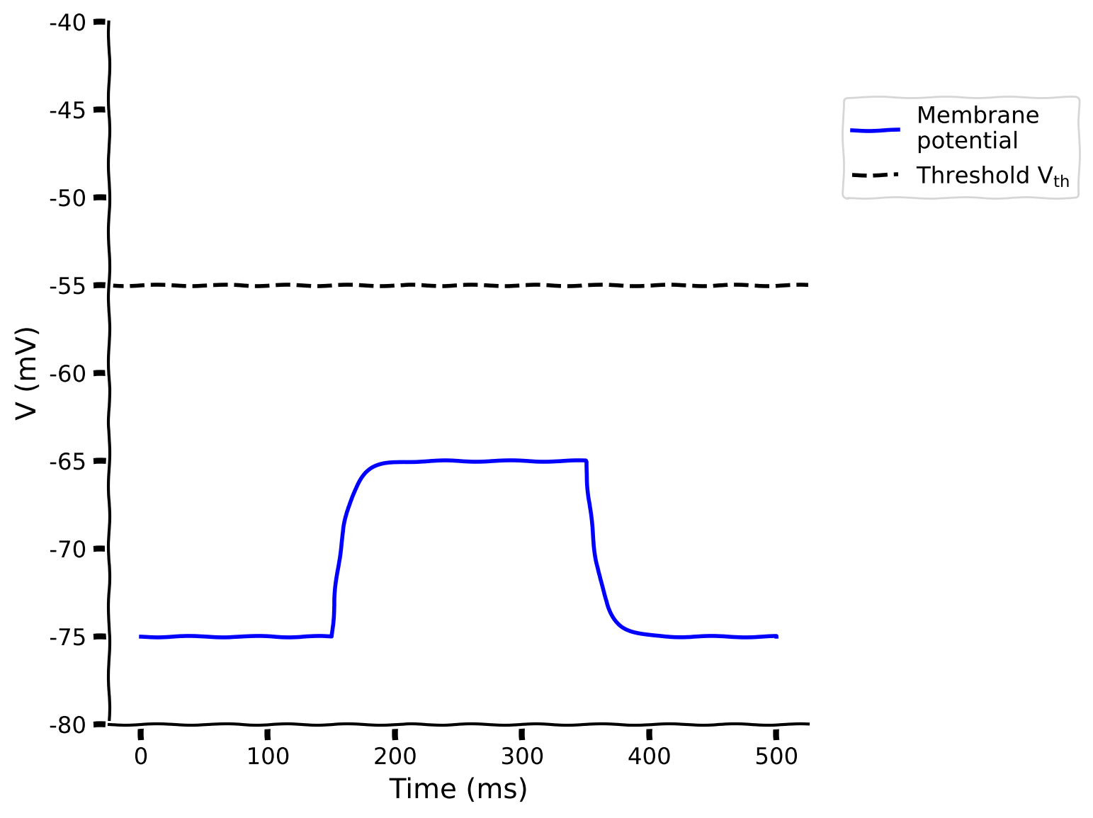
print(pars)

以下の関数を完成させて、外部電流入力を受けるLIFニューロンをシミュレートしてください。辞書parsと入力電流Iinjを与えると、膜電位(v)とスパイク列(sp)を得るためにv, sp = run_LIF(pars, Iinj)を使えます。

def run_LIF(pars, Iinj, stop=False):
  """
  Simulate the LIF dynamics with external input current

  Args:
    pars       : parameter dictionary
    Iinj       : input current [pA]. The injected current here can be a value
                 or an array
    stop       : boolean. If True, use a current pulse

  Returns:
    rec_v      : membrane potential
    rec_sp     : spike times
  """

  # Set parameters
  V_th, V_reset = pars['V_th'], pars['V_reset']
  tau_m, g_L = pars['tau_m'], pars['g_L']
  V_init, E_L = pars['V_init'], pars['E_L']
  dt, range_t = pars['dt'], pars['range_t']
  Lt = range_t.size
  tref = pars['tref']

  # Initialize voltage
  v = np.zeros(Lt)
  v[0] = V_init

  # Set current time course
  Iinj = Iinj * np.ones(Lt)

  # If current pulse, set beginning and end to 0
  if stop:
    Iinj[:int(len(Iinj) / 2) - 1000] = 0
    Iinj[int(len(Iinj) / 2) + 1000:] = 0

  # Loop over time
  rec_spikes = []  # record spike times
  tr = 0.  # the count for refractory duration

  for it in range(Lt - 1):

    if tr > 0:  # check if in refractory period
      v[it] = V_reset  # set voltage to reset
      tr = tr - 1 # reduce running counter of refractory period

    elif v[it] >= V_th:  # if voltage over threshold
      rec_spikes.append(it)  # record spike event
      v[it] = V_reset  # reset voltage
      tr = tref / dt  # set refractory time

    ########################################################################
    ## TODO for students: compute the membrane potential v, spike train sp #
    # Fill out function and remove
    raise NotImplementedError('Student Exercise: calculate the dv/dt and the update step!')
    ########################################################################

    # Calculate the increment of the membrane potential
    dv = ...

    # Update the membrane potential
    v[it + 1] = ...

  # Get spike times in ms
  rec_spikes = np.array(rec_spikes) * dt

  return v, rec_spikes


# Get parameters
pars = default_pars(T=500)

# Simulate LIF model
v, sp = run_LIF(pars, Iinj=100, stop=True)

# Visualize
plot_volt_trace(pars, v, sp)

解答を見る$

出力例:

# @title Submit your feedback
content_review(f"{feedback_prefix}_LIF_model_Exercise")

セクション2: LIFモデルの異なるタイプの入力電流に対する応答

チュートリアル開始からここまでの推定所要時間: 20分

以下のセクションでは、直接電流と白色雑音を注入してLIFニューロンの応答を学びます。

# @title Video 2: Response of the LIF neuron to different inputs
from ipywidgets import widgets
from IPython.display import YouTubeVideo
from IPython.display import IFrame
from IPython.display import display


class PlayVideo(IFrame):
  def __init__(self, id, source, page=1, width=400, height=300, **kwargs):
    self.id = id
    if source == 'Bilibili':
      src = f'https://player.bilibili.com/player.html?bvid={id}&page={page}'
    elif source == 'Osf':
      src = f'https://mfr.ca-1.osf.io/render?url=https://osf.io/download/{id}/?direct%26mode=render'
    super(PlayVideo, self).__init__(src, width, height, **kwargs)


def display_videos(video_ids, W=400, H=300, fs=1):
  tab_contents = []
  for i, video_id in enumerate(video_ids):
    out = widgets.Output()
    with out:
      if video_ids[i][0] == 'Youtube':
        video = YouTubeVideo(id=video_ids[i][1], width=W,
                             height=H, fs=fs, rel=0)
        print(f'Video available at https://youtube.com/watch?v={video.id}')
      else:
        video = PlayVideo(id=video_ids[i][1], source=video_ids[i][0], width=W,
                          height=H, fs=fs, autoplay=False)
        if video_ids[i][0] == 'Bilibili':
          print(f'Video available at https://www.bilibili.com/video/{video.id}')
        elif video_ids[i][0] == 'Osf':
          print(f'Video available at https://osf.io/{video.id}')
      display(video)
    tab_contents.append(out)
  return tab_contents


video_ids = [('Youtube', 'preNGdab7Kk'), ('Bilibili', 'BV1Li4y137wS')]
tab_contents = display_videos(video_ids, W=854, H=480)
tabs = widgets.Tab()
tabs.children = tab_contents
for i in range(len(tab_contents)):
  tabs.set_title(i, video_ids[i][0])
display(tabs)

# @title Submit your feedback
content_review(f"{feedback_prefix}_Response_LIF_model_Video")

セクション2.1: 直接電流（DC）

チュートリアル開始からここまでの推定所要時間: 30分

インタラクティブデモ2.1: DC入力振幅のパラメータ探索

これはDC入力（定常電流）の振幅を変えたときのLIFニューロンの挙動の変化を示すインタラクティブデモです。LIFニューロンの膜電位をプロットします。ニューロンがスパイクを発生するのが見えるかもしれませんが、これはあくまで見た目のスパイクで、LIFニューロンではニューロンが閾値に達した時刻だけを記録して、シナプス後ニューロンにスパイクを伝えます。

閾値に達するのに必要なDCの大きさ（レオベース電流）はどのくらいでしょうか？膜時定数はニューロンの発火頻度にどのように影響するでしょうか？

# @markdown Make sure you execute this cell to enable the widget!
my_layout.width = '450px'
@widgets.interact(
    I_dc=widgets.FloatSlider(50., min=0., max=300., step=10.,
                             layout=my_layout),
    tau_m=widgets.FloatSlider(10., min=2., max=20., step=2.,
                              layout=my_layout)
)

def diff_DC(I_dc=200., tau_m=10.):
  pars = default_pars(T=100.)
  pars['tau_m'] = tau_m
  v, sp = run_LIF(pars, Iinj=I_dc)
  plot_volt_trace(pars, v, sp)
  plt.show()

解答を見る$

# @title Submit your feedback
content_review(f"{feedback_prefix}_Parameter_exploration_of_DC_input_amplitude_Interactive_Demo_and_Discussion")

セクション2.2: ガウス白色雑音（GWN）電流

チュートリアル開始からここまでの推定所要時間: 38分

神経活動は_in vivo_ではノイズが多いため、ニューロンは通常複雑で時間変動する入力を受けています。

これを模倣するために、平均0（$\mu=0$）で標準偏差$\sigma$を持つガウス白色雑音$\xi(t)$をLIFニューロンに入力したときの応答を調べます。

GWNは平均0なので、ニューロンが受ける入力の変動のみを表します。したがって、平均値$\mu$を非ゼロにしてDC入力と等しくすることで、平均入力を持つ修正ガウス白色雑音を定義できます。以下のセルは非ゼロ平均$\mu$を持つ修正ガウス白色雑音電流を定義しています。

インタラクティブデモ2.2: ノイズ入力に対するLIFニューロンエクスプローラー

ガウス白色雑音（GWN）の平均はDCの振幅です。実際、$\sigma=0$のときGWNは単なるDCです。

ここで問題となるのは、GWNの$\sigma$がニューロンのスパイク挙動にどのように影響するかです。例えば以下のことを知りたいかもしれません。

1. ニューロンがスパイクするのに必要な最小入力（すなわち$\mu$）は$\sigma$の増加に伴いどう変わるか
2. スパイクの規則性は$\sigma$の増加に伴いどう変わるか

これらの直感を得るために、以下のインタラクティブデモを使って、異なる平均$\mu$と変動幅$\sigma$のノイズ入力に対するLIFニューロンの挙動の変化を示します。ノイズ入力電流はヘルパー関数my_GWN(pars, mu, sig, myseed=False)で生成します。乱数シードを固定（例:myseed=2020）すると毎回同じ結果が得られます。次にrun_LIF関数でLIFモデルをシミュレートします。

# @markdown Execute to enable helper function `my_GWN`

def my_GWN(pars, mu, sig, myseed=False):
  """
  Function that generates Gaussian white noise input

  Args:
    pars       : parameter dictionary
    mu         : noise baseline (mean)
    sig        : noise amplitute (standard deviation)
    myseed     : random seed. int or boolean
                 the same seed will give the same
                 random number sequence

  Returns:
    I          : Gaussian white noise input
  """

  # Retrieve simulation parameters
  dt, range_t = pars['dt'], pars['range_t']
  Lt = range_t.size

  # Set random seed
  if myseed:
      np.random.seed(seed=myseed)
  else:
      np.random.seed()

  # Generate GWN
  # we divide here by 1000 to convert units to sec.
  I_gwn = mu + sig * np.random.randn(Lt) / np.sqrt(dt / 1000.)

  return I_gwn

help(my_GWN)

# @markdown Make sure you execute this cell to enable the widget!

my_layout.width = '450px'
@widgets.interact(
    mu_gwn=widgets.FloatSlider(200., min=100., max=300., step=5.,
                               layout=my_layout),
    sig_gwn=widgets.FloatSlider(2.5, min=0., max=5., step=.5,
                                layout=my_layout)
)


def diff_GWN_to_LIF(mu_gwn, sig_gwn):
  pars = default_pars(T=100.)
  I_GWN = my_GWN(pars, mu=mu_gwn, sig=sig_gwn)
  v, sp = run_LIF(pars, Iinj=I_GWN)
  plt.figure(figsize=(12, 4))
  plt.subplot(121)
  plt.plot(pars['range_t'][::3], I_GWN[::3], 'b')
  plt.xlabel('Time (ms)')
  plt.ylabel(r'$I_{GWN}$ (pA)')
  plt.subplot(122)
  plot_volt_trace(pars, v, sp)
  plt.tight_layout()
  plt.show()

解答を見る$

# @title Submit your feedback
content_review(f"{feedback_prefix}_Gaussian_White_Noise_Interactive_Demo_and_Discussion")

考えてみよう！2.2：GWNがスパイクに与える影響の解析

• 入力の平均値（$\mu$）や入力の変動（$\sigma$）を増やすと、スパイク数はどう変化するでしょうか？スパイク数はどのくらい増やせるでしょうか？また、GWNの平均値・標準偏差やDC値とスパイク数の関係はどのようなものでしょうか？

• 先ほど見たように、DCを注入するとニューロンは規則的（時計のように）にスパイクしますが、GWNを注入するとこの規則性は減少します。GWNのパラメータを変えることで、ニューロンのスパイクの不規則性はどの程度まで高められるでしょうか？

これらの疑問の答えは次のセクションで見ていきますが、まずは議論してみましょう！

# @title Submit your feedback
content_review(f"{feedback_prefix}_Analyzing_GWN_effects_on_spiking_Discussion")

セクション3：発火率とスパイク時間の不規則性

チュートリアル開始からここまでの推定所要時間：48分

出力の発火率をGWNの平均値やDC値の関数としてプロットしたものは、ニューロンの入力-出力伝達関数（単にF-I曲線）と呼ばれます。

スパイクの規則性は、**スパイク間隔（ISI）の変動係数（CV）**で定量化できます：

ポアソン列は高い不規則性の例であり、$\textbf{CV}_{\textbf{ISI}} \textbf{= 1}$となります。一方、時計のように規則的な過程では、$\textbf{CV}_{\textbf{ISI}} \textbf{= 0}$となり、これはstd(ISI)=0であるためです。

インタラクティブデモ3A：異なるsig_gwnにおけるF-Iエクスプローラー

GWNの$\sigma$を増やすと、LIFニューロンのF-I曲線はどのように変化するでしょうか？F-I曲線は確率的になり、試行ごとに結果が異なることは予想できますが、DCを用いたF-I曲線と比べて他にどんな変化があるでしょうか？

以下は、変動の大きさ$\sigma$が異なる場合のLIFニューロンのF-I曲線の変化を示すインタラクティブデモです。

# @markdown Make sure you execute this cell to enable the widget!

my_layout.width = '450px'
@widgets.interact(
    sig_gwn=widgets.FloatSlider(3.0, min=0., max=6., step=0.5,
                                layout=my_layout)
)


def diff_std_affect_fI(sig_gwn):
  pars = default_pars(T=1000.)
  I_mean = np.arange(100., 400., 10.)
  spk_count = np.zeros(len(I_mean))
  spk_count_dc = np.zeros(len(I_mean))

  for idx in range(len(I_mean)):
      I_GWN = my_GWN(pars, mu=I_mean[idx], sig=sig_gwn, myseed=2020)
      v, rec_spikes = run_LIF(pars, Iinj=I_GWN)
      v_dc, rec_sp_dc = run_LIF(pars, Iinj=I_mean[idx])
      spk_count[idx] = len(rec_spikes)
      spk_count_dc[idx] = len(rec_sp_dc)

  # Plot the F-I curve i.e. Output firing rate as a function of input mean.
  plt.figure()
  plt.plot(I_mean, spk_count, 'k',
           label=r'$\sigma_{\mathrm{GWN}}=%.2f$' % sig_gwn)
  plt.plot(I_mean, spk_count_dc, 'k--', alpha=0.5, lw=4, dashes=(2, 2),
           label='DC input')
  plt.ylabel('Spike count')
  plt.xlabel('Average injected current (pA)')
  plt.legend(loc='best')
  plt.show()

解答を見る$

# @title Submit your feedback
content_review(f"{feedback_prefix}_F_I_explorer_Interactive_Demo_and_Discussion")

コーディング演習3：$CV_{ISI}$の計算

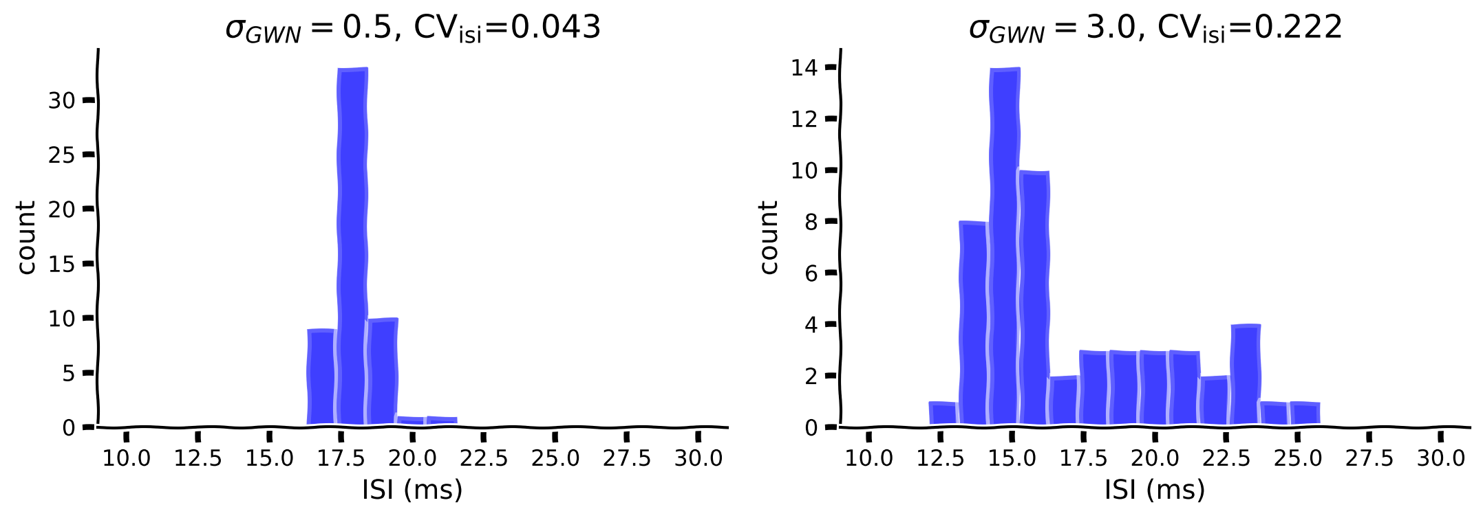
上記のように、変動の振幅（$\sigma$）を増やすとF-I曲線は滑らかになります。さらに、変動はスパイクの不規則性も変化させます。$\mu=250$で$\sigma=0.5$と$\sigma=3$の場合の影響を調べてみましょう。

以下のコードを完成させてISIを計算し、ISIのヒストグラムをプロットし、$CV_{ISI}$を計算してください。ISIの計算にはnp.diffを使えます。

def isi_cv_LIF(spike_times):
  """
  Calculates the interspike intervals (isi) and
  the coefficient of variation (cv) for a given spike_train

  Args:
    spike_times : (n, ) vector with the spike times (ndarray)

  Returns:
    isi         : (n-1,) vector with the inter-spike intervals (ms)
    cv          : coefficient of variation of isi (float)

  """
  ########################################################################
  ## TODO for students: compute the membrane potential v, spike train sp #
  # Fill out function and remove
  raise NotImplementedError('Student Exercise: calculate the isi and the cv!')
  ########################################################################
  if len(spike_times) >= 2:
    # Compute isi
    isi = ...
    # Compute cv
    cv = ...
  else:
    isi = np.nan
    cv = np.nan

  return isi, cv


# Set parameters
pars = default_pars(T=1000.)
mu_gwn = 250
sig_gwn1 = 0.5
sig_gwn2 = 3.0

# Run LIF model for sigma = 0.5
I_GWN1 = my_GWN(pars, mu=mu_gwn, sig=sig_gwn1, myseed=2020)
_, sp1 = run_LIF(pars, Iinj=I_GWN1)

# Run LIF model for sigma = 3
I_GWN2 = my_GWN(pars, mu=mu_gwn, sig=sig_gwn2, myseed=2020)
_, sp2 = run_LIF(pars, Iinj=I_GWN2)

# Compute ISIs/CV
isi1, cv1 = isi_cv_LIF(sp1)
isi2, cv2 = isi_cv_LIF(sp2)

# Visualize
my_hists(isi1, isi2, cv1, cv2, sig_gwn1, sig_gwn2)

解答を見る$

出力例:

# @title Submit your feedback
content_review(f"{feedback_prefix}_Compute_CV_ISI_Exercise")

インタラクティブデモ3B：異なるsig_gwnにおけるスパイク不規則性エクスプローラー

上の図から、スパイク間隔（ISI）のCVはGWNの$\sigma$に依存することがわかります。では、GWNの平均値はCV$_{\rm ISI}$に影響を与えるでしょうか？もしそうなら、どのように影響するでしょうか？また、CV$_{\rm ISI}$を増加させる$\sigma$の効果は$\mu$に依存するでしょうか？

以下のインタラクティブデモでは、異なる平均注入電流（$\mu$）に対して変動の大きさ$\sigma$がCVにどのように影響するかを調べます。

1. 注入電流の標準偏差はF-I曲線にどのような質的変化をもたらしますか？
2. なぜGWNの平均値を増やすとCV$_{\rm ISI}$が減少するのでしょうか？
3. スパイク数（または発火率）とCV$_{\rm ISI}$をプロットすると、両者の間に関係はあるでしょうか？自分で試してみましょう。

# @markdown Make sure you execute this cell to enable the widget!

my_layout.width = '450px'
@widgets.interact(
    sig_gwn=widgets.FloatSlider(0.0, min=0., max=10.,
                                step=0.5, layout=my_layout)
)


def diff_std_affect_fI(sig_gwn):
  pars = default_pars(T=1000.)
  I_mean = np.arange(100., 400., 20)
  spk_count = np.zeros(len(I_mean))
  cv_isi = np.empty(len(I_mean))

  for idx in range(len(I_mean)):
    I_GWN = my_GWN(pars, mu=I_mean[idx], sig=sig_gwn)
    v, rec_spikes = run_LIF(pars, Iinj=I_GWN)
    spk_count[idx] = len(rec_spikes)
    if len(rec_spikes) > 3:
      isi = np.diff(rec_spikes)
      cv_isi[idx] = np.std(isi) / np.mean(isi)

  # Plot the F-I curve i.e. Output firing rate as a function of input mean.
  plt.figure()
  plt.plot(I_mean[spk_count > 5], cv_isi[spk_count > 5], 'bo', alpha=0.5)
  plt.xlabel('Average injected current (pA)')
  plt.ylabel(r'Spike irregularity ($\mathrm{CV}_\mathrm{ISI}$)')
  plt.ylim(-0.1, 1.5)
  plt.grid(True)
  plt.show()

解答を見る$

# @title Submit your feedback
content_review(f"{feedback_prefix}_Spike_Irregularity_Interactive_Demo_and_Discussion")

まとめ

チュートリアルの推定所要時間：1時間10分

おめでとうございます！LIF（リーキー積分発火）ニューロンモデルを一から構築し、様々な入力に対する動的応答を学びました。

• LIFニューロンモデルのシミュレーション

• 直流電流やガウスホワイトノイズなどの外部入力による駆動

• 入力の違いがLIFニューロンの出力（発火率やスパイク時間の不規則性）に与える影響の検討

特に、実際の皮質ニューロンを模倣するために低発火率かつ不規則な発火状態に注目しました。次のチュートリアルでは、ニューロンの入力統計がスパイク統計にどのように影響するかを見ていきます。

時間に余裕があれば、以下のボーナスセクションで異なるタイプのノイズ入力や積分発火モデルの拡張について学んでみてください。

ボーナス

ボーナスセクション1：オーンシュタイン・ウーレンベック過程

ニューロンがスパイク入力を受けると、シナプス電流はショットノイズとなります。これは一種のカラー（有色）ノイズであり、ノイズのスペクトルはシナプスカーネルの時定数によって決まります。つまり、ニューロンはガウスホワイトノイズ（GWN）ではなくカラー（有色）ノイズによって駆動されます。

カラー（有色）ノイズはオーンシュタイン・ウーレンベック（OU）過程でモデル化できます。これはフィルタリングされたホワイトノイズです。

次に、入力電流が時間的に相関を持ち、オーンシュタイン・ウーレンベック過程$\eta(t)$としてモデル化される場合を考えます。これは時定数$\tau_{\eta}$を持つ低域通過フィルタをかけたGWNです：

ヒント： 上記のOU過程は以下の性質を持ちます。

および自己共分散

これらはコードの検証に使えます。

# @markdown Execute this cell to get helper function `my_OU`


def my_OU(pars, mu, sig, myseed=False):
  """
  Function that produces Ornstein-Uhlenbeck input

  Args:
    pars       : parameter dictionary
    sig        : noise amplitute
    myseed     : random seed. int or boolean

  Returns:
    I_ou       : Ornstein-Uhlenbeck input current
  """

  # Retrieve simulation parameters
  dt, range_t = pars['dt'], pars['range_t']
  Lt = range_t.size
  tau_ou = pars['tau_ou']  # [ms]

  # set random seed
  if myseed:
    np.random.seed(seed=myseed)
  else:
    np.random.seed()

  # Initialize
  noise = np.random.randn(Lt)
  I_ou = np.zeros(Lt)
  I_ou[0] = noise[0] * sig

  # generate OU
  for it in range(Lt-1):
    I_ou[it+1] = I_ou[it] + (dt / tau_ou) * (mu - I_ou[it]) + np.sqrt(2 * dt / tau_ou) * sig * noise[it + 1]

  return I_ou


help(my_OU)

ボーナスインタラクティブデモ1：OU入力を用いたLIFエクスプローラー

以下では、OU過程の統計に従うノイズ電流に対してニューロンがどのように応答するかを調べます。

• OUタイプの入力はニューロンの応答性をどのように変えるでしょうか？
• OU過程の時定数を増減させると、スパイクパターンや発火率はどう変わると思いますか？

# @markdown Remember to enable the widget by running the cell!

my_layout.width = '450px'
@widgets.interact(
  tau_ou=widgets.FloatSlider(10.0, min=5., max=20.,
                             step=2.5, layout=my_layout),
  sig_ou=widgets.FloatSlider(10.0, min=5., max=40.,
                             step=2.5, layout=my_layout),
  mu_ou=widgets.FloatSlider(190.0, min=180., max=220.,
                            step=2.5, layout=my_layout)
)


def LIF_with_OU(tau_ou=10., sig_ou=40., mu_ou=200.):
  pars = default_pars(T=1000.)
  pars['tau_ou'] = tau_ou  # [ms]

  I_ou = my_OU(pars, mu_ou, sig_ou)
  v, sp = run_LIF(pars, Iinj=I_ou)

  plt.figure(figsize=(12, 4))
  plt.subplot(121)
  plt.plot(pars['range_t'], I_ou, 'b', lw=1.0)
  plt.xlabel('Time (ms)')
  plt.ylabel(r'$I_{\mathrm{OU}}$ (pA)')
  plt.subplot(122)
  plot_volt_trace(pars, v, sp)
  plt.tight_layout()
  plt.show()

解答を見る$

# @title Submit your feedback
content_review(f"{feedback_prefix}_LIF_explorer_with_OU_input_Bonus_Interactive_Demo_and_Discussion")

ボーナスセクション2：一般化積分発火モデル

LIFモデルは実際のニューロンの唯一の抽象化ではありません。より現実的なニューロンモデルについて学びたい場合は、ボーナスビデオをご覧ください。

# @title Video 3 (Bonus): Extensions to Integrate-and-Fire models
from ipywidgets import widgets
from IPython.display import YouTubeVideo
from IPython.display import IFrame
from IPython.display import display


class PlayVideo(IFrame):
  def __init__(self, id, source, page=1, width=400, height=300, **kwargs):
    self.id = id
    if source == 'Bilibili':
      src = f'https://player.bilibili.com/player.html?bvid={id}&page={page}'
    elif source == 'Osf':
      src = f'https://mfr.ca-1.osf.io/render?url=https://osf.io/download/{id}/?direct%26mode=render'
    super(PlayVideo, self).__init__(src, width, height, **kwargs)


def display_videos(video_ids, W=400, H=300, fs=1):
  tab_contents = []
  for i, video_id in enumerate(video_ids):
    out = widgets.Output()
    with out:
      if video_ids[i][0] == 'Youtube':
        video = YouTubeVideo(id=video_ids[i][1], width=W,
                             height=H, fs=fs, rel=0)
        print(f'Video available at https://youtube.com/watch?v={video.id}')
      else:
        video = PlayVideo(id=video_ids[i][1], source=video_ids[i][0], width=W,
                          height=H, fs=fs, autoplay=False)
        if video_ids[i][0] == 'Bilibili':
          print(f'Video available at https://www.bilibili.com/video/{video.id}')
        elif video_ids[i][0] == 'Osf':
          print(f'Video available at https://osf.io/{video.id}')
      display(video)
    tab_contents.append(out)
  return tab_contents


video_ids = [('Youtube', 'G0b6wLhuQxE'), ('Bilibili', 'BV1c54y1B7d7')]
tab_contents = display_videos(video_ids, W=854, H=480)
tabs = widgets.Tab()
tabs.children = tab_contents
for i in range(len(tab_contents)):
  tabs.set_title(i, video_ids[i][0])
display(tabs)

# @title Submit your feedback
content_review(f"{feedback_prefix}_Extension_to_Integrate_and_Fire_Bonus_Video")