チュートリアル 4: 自己回帰モデル

第2週、第3日目：線形システム

Neuromatch Academyによる

コンテンツ作成者: Bing Wen Brunton, Biraj Pandey

コンテンツレビュアー: Norma Kuhn, John Butler, Matthew Krause, Ella Batty, Richard Gao, Michael Waskom

ポストプロダクションチーム: Gagana B, Spiros Chavlis

チュートリアルの目的

推定所要時間：30分

このチュートリアルの目的は、これまでのチュートリアルで開発したモデリングツールと直感を使って、_データにフィットさせる_ことです。コンセプトは前回のチュートリアルを逆にすることです。つまり、既知の基礎過程から合成データ点を生成するのではなく、時間で測定されたデータ点が与えられたときに、その基礎過程を学習するにはどうすればよいか、ということです。

このチュートリアルは2つのセクションに分かれています。

セクション1では、チュートリアル3のOU過程の係数をデータの回帰を用いて解く方法を説明します。次に、セクション2ではこの自己回帰フレームワークを高次の自己回帰モデルに一般化し、猿がタイプライターで打ったデータにフィットさせてみます。

# @title Tutorial slides
# @markdown These are the slides for the videos in all tutorials today
from IPython.display import IFrame
link_id = "snv4m"
print(f"If you want to download the slides: https://osf.io/download/{link_id}/")
IFrame(src=f"https://mfr.ca-1.osf.io/render?url=https://osf.io/{link_id}/?direct%26mode=render%26action=download%26mode=render", width=854, height=480)

セットアップ

# @title Install and import feedback gadget


from vibecheck import DatatopsContentReviewContainer
def content_review(notebook_section: str):
    return DatatopsContentReviewContainer(
        "",  # No text prompt
        notebook_section,
        {
            "url": "https://pmyvdlilci.execute-api.us-east-1.amazonaws.com/klab",
            "name": "neuromatch_cn",
            "user_key": "y1x3mpx5",
        },
    ).render()


feedback_prefix = "W2D2_T4"

# Imports
import numpy as np
import matplotlib.pyplot as plt

# @title Figure settings
import logging
logging.getLogger('matplotlib.font_manager').disabled = True
import ipywidgets as widgets  # interactive display
%config InlineBackend.figure_format = 'retina'
plt.style.use("https://raw.githubusercontent.com/NeuromatchAcademy/course-content/main/nma.mplstyle")

# @title Plotting Functions

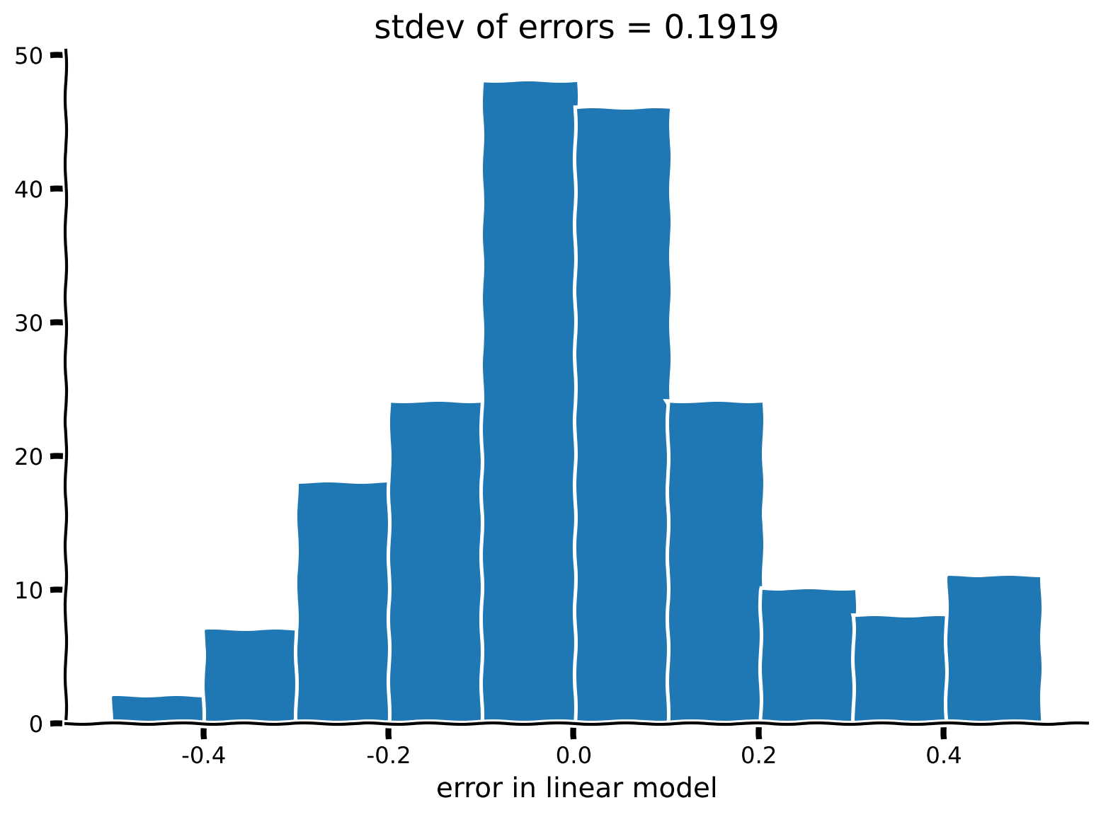
def plot_residual_histogram(res):
  """Helper function for Exercise 4A"""
  plt.figure()
  plt.hist(res)
  plt.xlabel('error in linear model')
  plt.title(f'stdev of errors = {res.std():.4f}')
  plt.show()


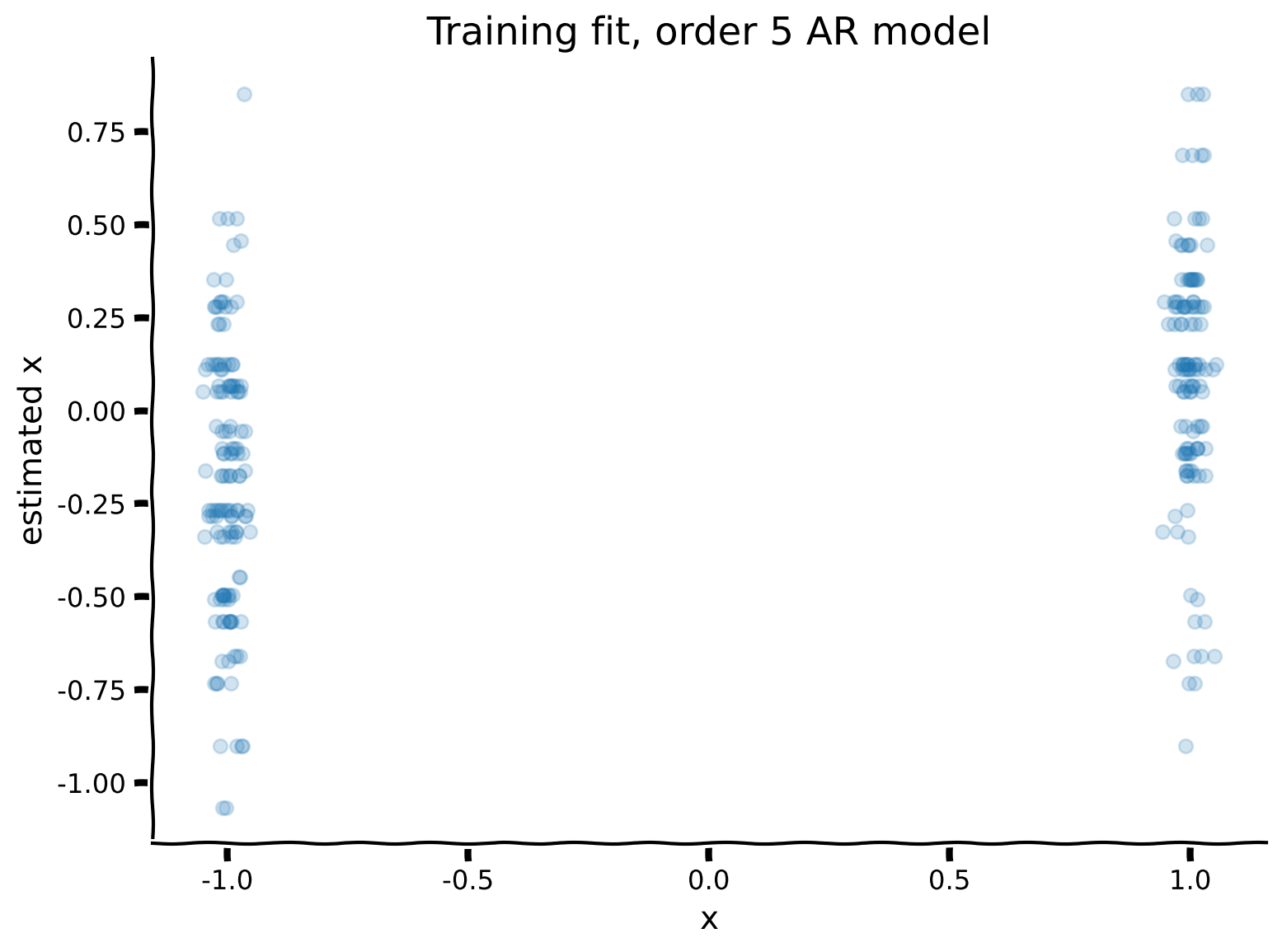
def plot_training_fit(x1, x2, p):
  """Helper function for Exercise 4B"""
  plt.figure()
  plt.scatter(x2 + np.random.standard_normal(len(x2))*0.02,
              np.dot(x1.T, p), alpha=0.2)
  plt.title(f'Training fit, order {r} AR model')
  plt.xlabel('x')
  plt.ylabel('estimated x')
  plt.show()

# @title Helper Functions

def ddm(T, x0, xinfty, lam, sig):
  '''
  Samples a trajectory of a drift-diffusion model.

  args:
  T (integer): length of time of the trajectory
  x0 (float): position at time 0
  xinfty (float): equilibrium position
  lam (float): process param
  sig: standard deviation of the normal distribution

  returns:
  t (numpy array of floats): time steps from 0 to T sampled every 1 unit
  x (numpy array of floats): position at every time step
  '''
  t = np.arange(0, T, 1.)
  x = np.zeros_like(t)
  x[0] = x0

  for k in range(len(t)-1):
      x[k+1] = xinfty + lam * (x[k] - xinfty) + sig * np.random.standard_normal(size=1)

  return t, x

def build_time_delay_matrices(x, r):
    """
    Builds x1 and x2 for regression

    Args:
    x (numpy array of floats): data to be auto regressed
    r (scalar): order of Autoregression model

    Returns:
    (numpy array of floats) : to predict "x2"
    (numpy array of floats) : predictors of size [r,n-r], "x1"

    """
    # construct the time-delayed data matrices for order-r AR model
    x1 = np.ones(len(x)-r)
    x1 = np.vstack((x1, x[0:-r]))
    xprime = x
    for i in range(r-1):
        xprime = np.roll(xprime, -1)
        x1 = np.vstack((x1, xprime[0:-r]))

    x2 = x[r:]

    return x1, x2


def AR_prediction(x_test, p):
    """
    Returns the prediction for test data "x_test" with the regression
    coefficients p

    Args:
    x_test (numpy array of floats): test data to be predicted
    p (numpy array of floats): regression coefficients of size [r] after
    solving the autoregression (order r) problem on train data

    Returns:
    (numpy array of floats): Predictions for test data. +1 if positive and -1
    if negative.
    """
    x1, x2 = build_time_delay_matrices(x_test, len(p)-1)

    # Evaluating the AR_model function fit returns a number.
    # We take the sign (- or +) of this number as the model's guess.
    return np.sign(np.dot(x1.T, p))

def error_rate(x_test, p):
    """
    Returns the error of the Autoregression model. Error is the number of
    mismatched predictions divided by total number of test points.

    Args:
    x_test (numpy array of floats): data to be predicted
    p (numpy array of floats): regression coefficients of size [r] after
    solving the autoregression (order r) problem on train data

    Returns:
    (float): Error (percentage).
    """
    x1, x2 = build_time_delay_matrices(x_test, len(p)-1)

    return np.count_nonzero(x2 - AR_prediction(x_test, p)) / len(x2)

セクション1: OU過程へのデータフィッティング

# @title Video 1: Autoregressive models
from ipywidgets import widgets
from IPython.display import YouTubeVideo
from IPython.display import IFrame
from IPython.display import display


class PlayVideo(IFrame):
  def __init__(self, id, source, page=1, width=400, height=300, **kwargs):
    self.id = id
    if source == 'Bilibili':
      src = f'https://player.bilibili.com/player.html?bvid={id}&page={page}'
    elif source == 'Osf':
      src = f'https://mfr.ca-1.osf.io/render?url=https://osf.io/download/{id}/?direct%26mode=render'
    super(PlayVideo, self).__init__(src, width, height, **kwargs)


def display_videos(video_ids, W=400, H=300, fs=1):
  tab_contents = []
  for i, video_id in enumerate(video_ids):
    out = widgets.Output()
    with out:
      if video_ids[i][0] == 'Youtube':
        video = YouTubeVideo(id=video_ids[i][1], width=W,
                             height=H, fs=fs, rel=0)
        print(f'Video available at https://youtube.com/watch?v={video.id}')
      else:
        video = PlayVideo(id=video_ids[i][1], source=video_ids[i][0], width=W,
                          height=H, fs=fs, autoplay=False)
        if video_ids[i][0] == 'Bilibili':
          print(f'Video available at https://www.bilibili.com/video/{video.id}')
        elif video_ids[i][0] == 'Osf':
          print(f'Video available at https://osf.io/{video.id}')
      display(video)
    tab_contents.append(out)
  return tab_contents


video_ids = [('Youtube', 'VdiVSTPbJ7I'), ('Bilibili', 'BV1fK4y1s7AQ')]
tab_contents = display_videos(video_ids, W=854, H=480)
tabs = widgets.Tab()
tabs.children = tab_contents
for i in range(len(tab_contents)):
  tabs.set_title(i, video_ids[i][0])
display(tabs)

# @title Submit your feedback
content_review(f"{feedback_prefix}_Autoregressive_models_Video")

この仕組みを理解するために、前回のドリフト拡散（OU）過程の例を続けましょう。我々の過程は以下の形をしていました：

x_{k+1} = x_{\infty} + \lambda(x_k - x_{\infty}) + \sigma \eta

ここで、 $\eta$ は標準正規分布からサンプリングされます。

簡単のために、 $x_\infty = 0$ と設定します。以下にこの過程の軌跡を再度プロットしましょう。パラメータに注目してください。後で重要になります。

# @markdown Execute to simulate the drift diffusion model
np.random.seed(2020) # set random seed

# parameters
T = 200
x0 = 10
xinfty = 0
lam = 0.9
sig = 0.2

# drift-diffusion model from tutorial 3
t, x = ddm(T, x0, xinfty, lam, sig)

plt.figure()
plt.title('$x_0=%d, x_{\infty}=%d, \lambda=%0.1f, \sigma=%0.1f$' % (x0, xinfty, lam, sig))
plt.plot(t, x, 'k.')
plt.xlabel('time')
plt.ylabel('position x')
plt.show()

もしこれらの位置 $x$ が時間とともに変化するデータとして与えられたら、システムの動力学 $\lambda$ をどうやって取り出すでしょうか？

このシステムが次の形を取ることは既にわかっています：

x_{k+1} = \lambda x_k + \eta \,,

ここで $\eta$ は正規分布のノイズです。したがって、我々のアプローチは $\lambda$ を回帰問題として解くことです。

確認のために、時間的に隣接するすべての点のペア（ $x_{k+1}$ 対 $x_k$ ）をプロットして、線形関係があるかどうかを見てみましょう。

# @markdown Execute to visualize X(k) vs. X(k+1)
# make a scatter plot of every data point in x
# at time k versus time k+1
plt.figure()
plt.scatter(x[0:-2], x[1:-1], color='k')
plt.plot([0, 10], [0, 10], 'k--', label='$x_{k+1} = x_k$ line')
plt.xlabel('$x_k$')
plt.ylabel('$x_{k+1}$')
plt.legend()
plt.show()

やった！直線になりました！これは、_データを生成した動力学_が線形である証拠です。これでこの課題を回帰問題として再定式化できます。

$\mathbf{x_1} = x_{0:T-1}$ と $\mathbf{x_2} = x_{1:T}$ を時間的に1ステップずらしたデータのベクトルとします。すると回帰問題は次のようになります：

\mathbf{x}_2 = \lambda \mathbf{x}_1

このモデルは自己回帰モデルで、auto は「自己」を意味します。つまり、過去の時系列自身に対する回帰です。上の式は過去の_1ステップ_だけに依存しているので、これは_一次_自己回帰モデルと呼べます。

では、以下で回帰問題を設定し、 $\lambda$ を解いてみましょう。データと回帰直線をプロットして一致を確認します。

# @markdown Execute to solve for lambda through autoregression
# build the two data vectors from x
x1 = x[0:-2]
x1 = x1[:, np.newaxis]**[0, 1]

x2 = x[1:-1]

# solve for an estimate of lambda as a linear regression problem
p, res, rnk, s = np.linalg.lstsq(x1, x2, rcond=None)

# here we've artificially added a vector of 1's to the x1 array,
# so that our linear regression problem has an intercept term to fit.
# we expect this coefficient to be close to 0.
# the second coefficient in the regression is the linear term:
# that's the one we're after!
lam_hat = p[1]

# plot the data points
fig = plt.figure()
plt.scatter(x[0:-2], x[1:-1], color='k')
plt.xlabel('$x_k$')
plt.ylabel('$x_{k+1}$')

# plot the 45 degree line
plt.plot([0, 10], [0, 10], 'k--', label='$x_{k+1} = x_k$ line')


# plot the regression line on top
xx = np.linspace(-sig*10, max(x), 100)
yy = p[0] + lam_hat * xx
plt.plot(xx, yy, 'r', linewidth=2, label='regression line')

mytitle = 'True $\lambda$ = {lam:.4f}, Estimate $\lambda$ = {lam_hat:.4f}'
plt.title(mytitle.format(lam=lam, lam_hat=lam_hat))
plt.legend()
plt.show()

すごいですね！これで任意のデータ点 $x_k$ が与えられたときに $x_{k+1}$ を予測する方法ができました。残差をプロットして、この1ステップ予測の精度を見てみましょう。

コーディング演習1: 自己回帰モデルの残差

動画内では演習4Aとして言及されています

自己回帰モデルの残差のヒストグラムをプロットしてください。残差は_データ_ $\mathbf{x_2}$ と_モデル_の予測の差です。この残差の標準偏差と、この合成データセットを生成した方程式について何か気づきますか？

##############################################################################
## Insert your code here take to compute the residual (error)
raise NotImplementedError('student exercise: compute the residual error')
##############################################################################
# compute the predicted values using the autoregressive model (lam_hat), and
# the residual is the difference between x2 and the prediction
res = ...

# Visualize
plot_residual_histogram(res)

解答を見る$

出力例:

# @title Submit your feedback
content_review(f"{feedback_prefix}_Residuals_of_the_autoregressive_model_Exercise")

セクション2: 高次自己回帰モデル

チュートリアル開始からここまでの推定所要時間：15分

# @title Video 2: Monkey at a typewriter
from ipywidgets import widgets
from IPython.display import YouTubeVideo
from IPython.display import IFrame
from IPython.display import display


class PlayVideo(IFrame):
  def __init__(self, id, source, page=1, width=400, height=300, **kwargs):
    self.id = id
    if source == 'Bilibili':
      src = f'https://player.bilibili.com/player.html?bvid={id}&page={page}'
    elif source == 'Osf':
      src = f'https://mfr.ca-1.osf.io/render?url=https://osf.io/download/{id}/?direct%26mode=render'
    super(PlayVideo, self).__init__(src, width, height, **kwargs)


def display_videos(video_ids, W=400, H=300, fs=1):
  tab_contents = []
  for i, video_id in enumerate(video_ids):
    out = widgets.Output()
    with out:
      if video_ids[i][0] == 'Youtube':
        video = YouTubeVideo(id=video_ids[i][1], width=W,
                             height=H, fs=fs, rel=0)
        print(f'Video available at https://youtube.com/watch?v={video.id}')
      else:
        video = PlayVideo(id=video_ids[i][1], source=video_ids[i][0], width=W,
                          height=H, fs=fs, autoplay=False)
        if video_ids[i][0] == 'Bilibili':
          print(f'Video available at https://www.bilibili.com/video/{video.id}')
        elif video_ids[i][0] == 'Osf':
          print(f'Video available at https://osf.io/{video.id}')
      display(video)
    tab_contents.append(out)
  return tab_contents


video_ids = [('Youtube', 'f2z0eopWB8Y'), ('Bilibili', 'BV1si4y1V7Ru')]
tab_contents = display_videos(video_ids, W=854, H=480)
tabs = widgets.Tab()
tabs.children = tab_contents
for i in range(len(tab_contents)):
  tabs.set_title(i, video_ids[i][0])
display(tabs)

# @title Submit your feedback
content_review(f"{feedback_prefix}_Monkey_at_a_typewriter_Video")

自己回帰フレームワークが確立できたので、過去の複数のデータ点に依存するモデルへの一般化は簡単です。高次自己回帰モデルは、未来の時点を過去の_複数の点_に基づいてモデル化します。

1次元の場合、次数 $r$ のモデルは次のように書けます：

x_{k+1} = \alpha_0 + \alpha_1 x_k + \alpha_2 x_{k-1} + \alpha_3 x_{k-2} + \dots + \alpha_{r+1} x_{k-r} \, ,

ここで $\alpha$ はデータにフィットさせる $r+1$ 個の係数です。

これらのモデルは時系列の軌跡における履歴依存性を考慮するのに有用です。次のパートでは、そうした時系列の一例を探求し、あなた自身で実験ができます！

具体的には、コインを投げてその結果を書き留めたときに得られる0と1の二値のランダム列を扱います。

違いは、実際にコインを投げる（あるいはコードで生成する）のではなく、あなた自身が0と1をできるだけランダムにタイプして、このベルヌーイ列を生成することです。次に、高次ARモデルを構築して、あなたが生成した数字の時系列の履歴に予測可能なパターンがあるかどうかを調べます。

まずは、単純なパターンの列で試してみて、フレームワークが機能していることを確認しましょう。以下では完全に予測可能な列を生成し、プロットしています。

# this sequence is entirely predictable, so an AR model should work
monkey_at_typewriter = '1010101010101010101010101010101010101010101010101'

# Bonus: this sequence is also predictable, but does an order-1 AR model work?
#monkey_at_typewriter = '100100100100100100100100100100100100100'

# function to turn chars to numpy array,
# coding it this way makes the math easier
# '0' -> -1
# '1' -> +1
def char2array(s):
  m = [int(c) for c in s]
  x = np.array(m)
  return x*2 - 1


x = char2array(monkey_at_typewriter)

plt.figure()
plt.step(x, '.-')
plt.xlabel('time')
plt.ylabel('random variable')
plt.show()

次に、上記のように1次自己回帰の回帰問題を設定し、 $\mathbf{x_1}$ と $\mathbf{x_2}$ を定義して解きます。

# build the two data vectors from x
x1 = x[0:-2]
x1 = x1[:, np.newaxis]**[0, 1]

x2 = x[1:-1]

# solve for an estimate of lambda as a linear regression problem
p, res, rnk, s = np.linalg.lstsq(x1, x2, rcond=None)

# take a look at the resulting regression coefficients
print(f'alpha_0 = {p[0]:.2f}, alpha_1 = {p[1]:.2f}')

考えてみよう！2: 自己回帰パラメータの理解

得られた $\alpha_0$ と $\alpha_1$ の値は妥当でしょうか？対応する自己回帰モデルを書き出し、交互に0と1が現れるパターンをうまく表現できていることを確認してください。

解答を見る$

# @title Submit your feedback
content_review(f"{feedback_prefix}_Understanding_autoregressive_parameters_Discussion")

真にランダムな数列には構造がなく、ARモデルや他のモデルで予測できるべきではありません。

しかし、人間はランダムな数列を生成するのが非常に苦手です！（他の動物も同様です…）

高次ARモデルの応用例として、人間がランダムに生成しようとした0と1の列をモデル化してみましょう。具体的には、私の9歳の猿（子供）がタイプライター（私のノートパソコン）に座って、できるだけランダムに数字を入力しました。その数字はコード内にあり、ここで時系列としてプロットします。

もし数字に本当に構造がなければ、モデルの誤差率は0.5（ランダム推測と同じ）になるはずです。どれくらい良くできるか見てみましょう！

# data generated by 9-yr-old JAB:
# we will be using this sequence to train the data
monkey_at_typewriter = '10010101001101000111001010110001100101000101101001010010101010001101101001101000011110100011011010010011001101000011101001110000011111011101000011110000111101001010101000111100000011111000001010100110101001011010010100101101000110010001100011100011100011100010110010111000101'

# we will be using this sequence to test the data
test_monkey = '00100101100001101001100111100101011100101011101001010101000010110101001010100011110'

x = char2array(monkey_at_typewriter)
test = char2array(test_monkey)

## testing: machine generated randint should be entirely unpredictable
## uncomment the lines below to try random numbers instead
# np.random.seed(2020) # set random seed
# x = char2array(np.random.randint(2, size=500))
# test = char2array(np.random.randint(2, size=500))

plt.figure()
plt.step(x, '.-')
plt.xlabel('time')
plt.ylabel('random variable')
plt.show()

コーディング演習2: ARモデルのフィッティング

動画内では演習4Bとして言及されています

データベクトル $x$ に対して5次（ $r=5$ ）のARモデルをフィットさせてください。補助関数 AR_model を用意しています。

その後、観測値と学習済みモデルの予測をプロットします。これは、直前の5つの数字の列を使って次の数字を予測することを意味します。

また、回帰モデルの出力は連続値（実数）ですが、データはスカラー（+1/-1）なので、連続値の符号（正なら+1、負なら-1）を予測値として使い、データと比較可能にします。誤差率は予測と実際の不一致数を予測総数で割ったものです。

# @markdown Execute this cell to get helper function `AR_model`

def AR_model(x, r):
    """
    Solves Autoregression problem of order (r) for x

    Args:
    x (numpy array of floats): data to be auto regressed
    r (scalar): order of Autoregression model

    Returns:
    (numpy array of floats) : to predict "x2"
    (numpy array of floats) : predictors of size [r,n-r], "x1"
    (numpy array of floats): coefficients of length [r] for prediction after
    solving the regression problem "p"
    """
    x1, x2 = build_time_delay_matrices(x, r)

    # solve for an estimate of lambda as a linear regression problem
    p, res, rnk, s = np.linalg.lstsq(x1.T, x2, rcond=None)

    return x1, x2, p

help(AR_model)

##############################################################################
## TODO: Insert your code here for fitting the AR model
raise NotImplementedError('student exercise: fit AR model')
##############################################################################
# define the model order, and use AR_model() to generate the model and prediction
r = ...
x1, x2, p = AR_model(...)

# Plot the Training data fit
# Note that this adds a small amount of jitter to horizontal axis for visualization purposes
plot_training_fit(x1, x2, p)

解答を見る$

出力例:

# @title Submit your feedback
content_review(f"{feedback_prefix}_Fitting_AR_models_Exercise")

モデルが見たことのないテストデータに対してどのように動作するか見てみましょう！

# @markdown Execute to see model performance on test data

x1_test, x2_test = build_time_delay_matrices(test, r)
plt.figure()
plt.scatter(x2_test+np.random.standard_normal(len(x2_test))*0.02,
            np.dot(x1_test.T, p), alpha=0.5)
mytitle = f'Testing fit, order {r} AR model, err = {error_rate(test, p):.3f}'
plt.title(mytitle)
plt.xlabel('test x')
plt.ylabel('estimated x')
plt.show()

悪くないですね！誤差は0.5（ランダム推測の誤差）より小さくなっています。

次に、異なる次数のARモデルを系統的に試し、それぞれのテスト誤差をプロットしましょう。

覚えておいてください：モデルはテストデータを見たことがなく、ランダム推測は誤差0.5を出します。

# @markdown Execute to visualize errors for different orders

# range of r's to try
r = np.arange(1, 21)
err = np.ones_like(r) * 1.0

for i, rr in enumerate(r):
  # fitting the model on training data
  x1, x2, p = AR_model(x, rr)
  # computing and storing the test error
  test_error = error_rate(test, p)
  err[i] = test_error


plt.figure()
plt.plot(r, err, '.-')
plt.plot([1, r[-1]], [0.5, 0.5], 'r--', label='random chance')
plt.xlabel('Order r of AR model')
plt.ylabel('Test error')
plt.xticks(np.arange(0,25,5))
plt.legend()
plt.show()

テスト誤差に最適なポイントがあることに気づきます！6次のARモデルが非常に良い結果を出し、それ以上の次数ではモデルが訓練データに過剰適合し、テストデータでの性能が落ちます。

まとめると：

「自分がこんなに予測可能だなんて信じられない！」 - JAB

まとめ

推定所要時間：30分

このチュートリアルで学んだこと：

線形動的システムのパラメータ学習は、データからの回帰問題として定式化できること。
時系列の履歴依存性は、回帰フレームワークにおける重回帰問題として組み込めること。
人間はランダム（予測不可能）な列を生成するのが苦手であること。ぜひ自分で試してみてください！