![]()

チュートリアル 3: 決定論と確率論の組み合わせ
第2週、第3日目: 線形システム
Neuromatch Academy 提供
コンテンツ作成者: Bing Wen Brunton, Alice Schwarze, Biraj Pandey
コンテンツレビュアー: Norma Kuhn, John Butler, Matthew Krause, Ella Batty, Richard Gao, Michael Waskom
制作編集者: Gagana B, Spiros Chavlis
チュートリアルの目標
チュートリアルの推定所要時間: 45分
時間依存のプロセスは世界を支配しています。
これまでに、軌道が (1) 完全に予測可能で決定論的である場合、または (2) ランダムなプロセスによって支配される場合のシステムの挙動に慣れてきましたが、どちらも神経科学を説明するには不十分であることがわかりました。代わりに、私たちはしばしば、いくつかの力学はわかっているが、同時にランダムな側面もあるプロセスに直面します。これを確率性を含む動的システムと呼びます。
このチュートリアルでは、決定論的プロセスと確率的プロセスの両方が動的システムの一部となる仕組みについての知識を深め、直感を養うために以下を行います:
- ランダムウォークのシミュレーション
- オーンシュタイン・ウーレンベック(OU)過程の平均と分散の調査
- 平衡状態におけるOU過程の挙動の定量化
# @title Tutorial slides
# @markdown These are the slides for the videos in all tutorials today
from IPython.display import IFrame
link_id = "snv4m"
print(f"If you want to download the slides: https://osf.io/download/{link_id}/")
IFrame(src=f"https://mfr.ca-1.osf.io/render?url=https://osf.io/{link_id}/?direct%26mode=render%26action=download%26mode=render", width=854, height=480)
セットアップ
# @title Install and import feedback gadget


from vibecheck import DatatopsContentReviewContainer
def content_review(notebook_section: str):
    return DatatopsContentReviewContainer(
        "",  # No text prompt
        notebook_section,
        {
            "url": "https://pmyvdlilci.execute-api.us-east-1.amazonaws.com/klab",
            "name": "neuromatch_cn",
            "user_key": "y1x3mpx5",
        },
    ).render()


feedback_prefix = "W2D2_T3"
# Imports
import numpy as np
import matplotlib.pyplot as plt# @title Figure Settings
import logging
logging.getLogger('matplotlib.font_manager').disabled = True
import ipywidgets as widgets # interactive display
%config InlineBackend.figure_format = 'retina'
plt.style.use("https://raw.githubusercontent.com/NeuromatchAcademy/course-content/main/nma.mplstyle")# @title Plotting Functions
def plot_random_walk_sims(sims, nsims=10):
"""Helper for exercise 3A"""
plt.figure()
plt.plot(sim[:nsims, :].T)
plt.xlabel('time')
plt.ylabel('position x')
plt.show()
def plot_mean_var_by_timestep(mu, var):
"""Helper function for exercise 3A.2"""
fig, (ah1, ah2) = plt.subplots(2)
# plot mean of distribution as a function of time
ah1.plot(mu)
ah1.set(ylabel='mean')
ah1.set_ylim([-5, 5])
# plot variance of distribution as a function of time
ah2.plot(var)
ah2.set(xlabel='time')
ah2.set(ylabel='variance')
plt.show()
def plot_ddm(t, x, xinfty, lam, x0):
plt.figure()
plt.plot(t, xinfty * (1 - lam**t) + x0 * lam**t, 'r',
label='deterministic solution')
plt.plot(t, x, 'k.', label='simulation') # simulated data pts
plt.xlabel('t')
plt.ylabel('x')
plt.legend()
plt.show()
def var_comparison_plot(empirical, analytical):
plt.figure()
plt.plot(empirical, analytical, '.', markersize=15)
plt.xlabel('empirical equilibrium variance')
plt.ylabel('analytic equilibrium variance')
plt.plot(np.arange(8), np.arange(8), 'k', label='45 deg line')
plt.legend()
plt.grid(True)
plt.show()
def plot_dynamics(x, t, lam, xinfty=0):
""" Plot the dynamics """
plt.figure()
plt.title('$\lambda=%0.1f$' % lam, fontsize=16)
x0 = x[0]
plt.plot(t, xinfty + (x0 - xinfty) * lam**t, 'r', label='analytic solution')
plt.plot(t, x, 'k.', label='simulation') # simulated data pts
plt.ylim(0, x0+1)
plt.xlabel('t')
plt.ylabel('x')
plt.legend()
plt.show()セクション1:ランダムウォーク
# @title Video 1: E. coli and Random Walks
from ipywidgets import widgets
from IPython.display import YouTubeVideo
from IPython.display import IFrame
from IPython.display import display


class PlayVideo(IFrame):
  def __init__(self, id, source, page=1, width=400, height=300, **kwargs):
    self.id = id
    if source == 'Bilibili':
      src = f'https://player.bilibili.com/player.html?bvid={id}&page={page}'
    elif source == 'Osf':
      src = f'https://mfr.ca-1.osf.io/render?url=https://osf.io/download/{id}/?direct%26mode=render'
    super(PlayVideo, self).__init__(src, width, height, **kwargs)


def display_videos(video_ids, W=400, H=300, fs=1):
  tab_contents = []
  for i, video_id in enumerate(video_ids):
    out = widgets.Output()
    with out:
      if video_ids[i][0] == 'Youtube':
        video = YouTubeVideo(id=video_ids[i][1], width=W,
                             height=H, fs=fs, rel=0)
        print(f'Video available at https://youtube.com/watch?v={video.id}')
      else:
        video = PlayVideo(id=video_ids[i][1], source=video_ids[i][0], width=W,
                          height=H, fs=fs, autoplay=False)
        if video_ids[i][0] == 'Bilibili':
          print(f'Video available at https://www.bilibili.com/video/{video.id}')
        elif video_ids[i][0] == 'Osf':
          print(f'Video available at https://osf.io/{video.id}')
      display(video)
    tab_contents.append(out)
  return tab_contents


video_ids = [('Youtube', 'VHwTBCQJjfw'), ('Bilibili', 'BV1LC4y1h7gD')]
tab_contents = display_videos(video_ids, W=854, H=480)
tabs = widgets.Tab()
tabs.children = tab_contents
for i in range(len(tab_contents)):
  tabs.set_title(i, video_ids[i][0])
display(tabs)
# @title Submit your feedback
content_review(f"{feedback_prefix}_Ecoli_and_Random_Walks_Video")まずは、人生が時に目的もなくさまよう様子を見てみましょう。最も単純でよく研究されている生物システムの一つに、基質上のにおいの勾配をたどって食物源を探すことができる大腸菌(E. coli)があります。ハエや犬、目隠しをした人間などのより大きな生物も、意思決定の指針として同じ戦略を使うことがあります。
ここでは、食物のにおいがない場合に大腸菌がどうするかを考えます。どこに向かえばよいかわからないときの最善の戦略は何でしょうか?もちろん、ランダムに動き回ることです!
ランダムウォークとはまさにそれで、各時間ステップでコインを投げるようなランダムな過程を用いて進行方向を決めます。この過程はブラウン運動と密接に関連しているため、時にその用語が使われることもあります。
まずは一次元ランダムウォークから始めましょう。細菌は位置からスタートします。各時間ステップでコインを投げ(非常に小さなタンパク質製のコインです)、左に、右にのいずれかに等確率で進みます。例えば、時間ステップ1でコインの結果が右なら、その時点の位置はとなります。このようにして、時間ステップでの位置は次のように表されます。
この過程を以下でシミュレーションし、細菌の位置を時間ステップの関数としてプロットします。
# @markdown Execute to simulate and visualize a random walk
# parameters of simulation
T = 100
t = np.arange(T)
x = np.zeros_like(t)
np.random.seed(2020) # set random seed

# initial position
x[0] = 0

# step forward in time
for k in range(len(t)-1):
    # choose randomly between -1 and 1 (coin flip)
    this_step = np.random.choice([-1,1])

    # make the step
    x[k+1] = x[k] + this_step

# plot this trajectory
plt.figure()
plt.step(t, x)
plt.xlabel('time')
plt.ylabel('position x')
plt.show()
コーディング演習1A:ランダムウォークのシミュレーション
動画内では演習3Aとして言及されています
前のプロットでは、細菌が各時点で1の大きさのステップを踏むと仮定しました。今度は異なる大きさのステップを踏ませてみましょう!
ステップが平均、標準偏差の正規分布に従うランダムウォークをコード化します。1つの軌跡を順に実行するのではなく、多数の軌跡を効率的にシミュレートできるようにコードを書きます。これらをまとめて、本のランダムウォークをそれぞれ時点で生成する関数random_walk_simulatorを作成します。
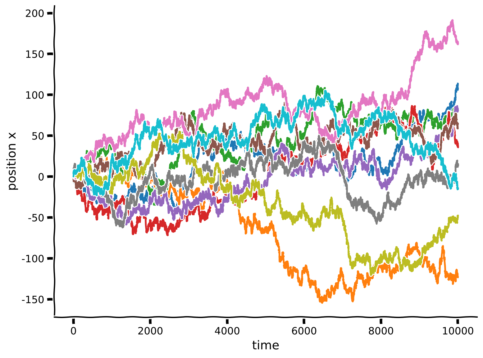
10000ステップのランダムウォークを10本プロットします。
def random_walk_simulator(N, T, mu=0, sigma=1):
  '''Simulate N random walks for T time points. At each time point, the step
      is drawn from a Gaussian distribution with mean mu and standard deviation
      sigma.

  Args:
    T (integer) : Duration of simulation in time steps
    N (integer) : Number of random walks
    mu (float) : mean of step distribution
    sigma (float) : standard deviation of step distribution

  Returns:
    (numpy array) : NxT array in which each row corresponds to trajectory
  '''

  ###############################################################################
  ## TODO: Code the simulated random steps to take
  ## Hints: you can generate all the random steps in one go in an N x T matrix
  raise NotImplementedError('Complete random_walk_simulator_function')
  ###############################################################################
  # generate all the random steps for all steps in all simulations in one go
  # produces a N x T array
  steps = np.random.normal(..., ..., size=(..., ...))

  # compute the cumulative sum of all the steps over the time axis
  sim = np.cumsum(steps, axis=1)

  return sim


np.random.seed(2020) # set random seed

# simulate 1000 random walks for 10000 time steps
sim = random_walk_simulator(1000, 10000,  mu=0, sigma=1)

# take a peek at the first 10 simulations
plot_random_walk_sims(sim, nsims=10)出力例:
# @title Submit your feedback
content_review(f"{feedback_prefix}_Random_Walk_simulation_Exercise")
軌跡はそれぞれ少しずつ異なって見えますが、いくつか一般的な観察ができます。最初はほとんどの軌跡が に非常に近く、これは細菌がスタートした位置です。時間が経つにつれて、いくつかの軌跡は出発点からどんどん離れていきます。しかし、多くの軌跡は の出発点の近くにとどまっています。
次のセルでは、先ほど生成したすべての軌跡を解析し、異なる時間点での細菌の位置の分布を見てみましょう。
# @markdown Execute to visualize distribution of bacteria positions
fig = plt.figure()
# look at the distribution of positions at different times
for i, t in enumerate([1000, 2500, 10000]):

  # get mean and standard deviation of distribution at time t
  mu = sim[:, t-1].mean()
  sig2 = sim[:, t-1].std()

  # make a plot label
  mytitle = '$t=${time:d} ($\mu=${mu:.2f}, $\sigma=${var:.2f})'

  # plot histogram
  plt.hist(sim[:,t-1],
           color=['blue','orange','black'][i],
           # make sure the histograms have the same bins!
           bins=np.arange(-300, 300, 20),
           # make histograms a little see-through
           alpha=0.6,
           # draw second histogram behind the first one
           zorder=3-i,
           label=mytitle.format(time=t, mu=mu, var=sig2))

  plt.xlabel('position x')

  # plot range
  plt.xlim([-500, 250])

  # add legend
  plt.legend(loc=2)

# add title
plt.title(r'Distribution of trajectory positions at time $t$')
plt.show()
シミュレーションの開始時点では、位置の分布は の周りに鋭くピークを持っています。時間が経つにつれて分布は広がりますが、その中心は に近いままです。言い換えれば、分布の平均は時間に依存しませんが、分布の分散と標準偏差は時間とともにスケールします。このような過程は拡散過程と呼ばれます。
コーディング演習 1B: ランダムウォークの平均と分散
細菌のランダムウォークの平均と分散を時間の関数として計算し、プロットしてください。
# Simulate random walks
np.random.seed(2020) # set random seed
sim = random_walk_simulator(5000, 1000, mu=0, sigma=1)

##############################################################################
# TODO: Insert your code here to compute the mean and variance of trajectory positions
# at every time point:
raise NotImplementedError("Student exercise: need to compute mean and variance")
##############################################################################

# Compute mean
mu = ...

# Compute variance
var = ...

# Visualize
plot_mean_var_by_timestep(mu, var)出力例:
# @title Submit your feedback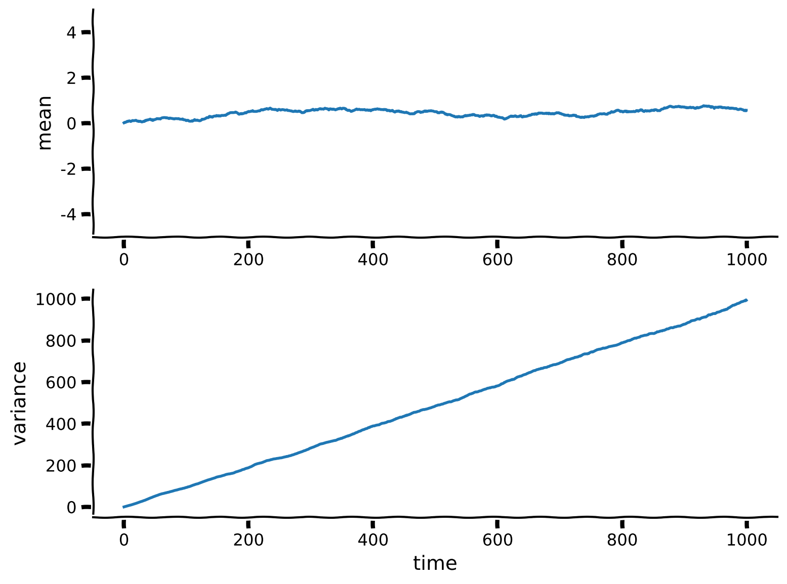
content_review(f"{feedback_prefix}_Random_Walk_and_variance_Exercise")の期待値は非常に長い時間のランダムウォークでもほぼ0のままです。すごいですね!
一方で分散は明らかに時間とともに増加しています。実際、分散は時間に比例して増加しているようです!
インタラクティブデモ 1: パラメータ選択の影響
細菌のランダムウォークのステップを選ぶ際のガウス分布のパラメータ と は、平均と分散にどのような影響を与えるでしょうか?
# @markdown Make sure you execute this cell to enable the widget!

@widgets.interact
def plot_gaussian(mean=(-0.5, 0.5, .02), std=(.5, 10, .5)):
  sim = random_walk_simulator(5000, 1000, mu=mean, sigma=std)
  # compute the mean and variance of trajectory positions at every time point
  mu = np.mean(sim, axis=0)
  var = np.var(sim, axis=0)
  # make a figure
  fig, (ah1, ah2) = plt.subplots(2)
  # plot mean of distribution as a function of time
  ah1.plot(mu)
  ah1.set(ylabel='mean')
  # plot variance of distribution as a function of time
  ah2.plot(var)
  ah2.set(xlabel='time')
  ah2.set(ylabel='variance')
plt.show()# @title Submit your feedback
content_review(f"{feedback_prefix}_Influence_of_Parameter_Choice_Interactive_Demo_and_Discussion")セクション2: オーンシュタイン-ウーレンベック(OU)過程
チュートリアル開始からここまでの推定所要時間: 14分
# @title Video 2: Combining Deterministic & Stochastic Processes
from ipywidgets import widgets
from IPython.display import YouTubeVideo
from IPython.display import IFrame
from IPython.display import display


class PlayVideo(IFrame):
  def __init__(self, id, source, page=1, width=400, height=300, **kwargs):
    self.id = id
    if source == 'Bilibili':
      src = f'https://player.bilibili.com/player.html?bvid={id}&page={page}'
    elif source == 'Osf':
      src = f'https://mfr.ca-1.osf.io/render?url=https://osf.io/download/{id}/?direct%26mode=render'
    super(PlayVideo, self).__init__(src, width, height, **kwargs)


def display_videos(video_ids, W=400, H=300, fs=1):
  tab_contents = []
  for i, video_id in enumerate(video_ids):
    out = widgets.Output()
    with out:
      if video_ids[i][0] == 'Youtube':
        video = YouTubeVideo(id=video_ids[i][1], width=W,
                             height=H, fs=fs, rel=0)
        print(f'Video available at https://youtube.com/watch?v={video.id}')
      else:
        video = PlayVideo(id=video_ids[i][1], source=video_ids[i][0], width=W,
                          height=H, fs=fs, autoplay=False)
        if video_ids[i][0] == 'Bilibili':
          print(f'Video available at https://www.bilibili.com/video/{video.id}')
        elif video_ids[i][0] == 'Osf':
          print(f'Video available at https://osf.io/{video.id}')
      display(video)
    tab_contents.append(out)
  return tab_contents


video_ids = [('Youtube', 'pDNfs5p38fI'), ('Bilibili', 'BV1o5411Y7N2')]
tab_contents = display_videos(video_ids, W=854, H=480)
tabs = widgets.Tab()
tabs.children = tab_contents
for i in range(len(tab_contents)):
  tabs.set_title(i, video_ids[i][0])
display(tabs)
# @title Submit your feedback
content_review(f"{feedback_prefix}_Combining_Deterministic_and_Stochastic_Processes_Video")先ほど調べたランダムウォーク過程は拡散的で、可能な軌跡の分布は時間とともに広がり、分散が増加します。それでも、少なくとも一次元では平均は初期値(上の例では0)に近いままです。
ここでの目標は、このモデルを基にして**ドリフト-拡散モデル(DDM)**を構築することです。DDMは記憶のための一般的なモデルであり、私たちが知っているように、記憶とはしばしば値を不完全に保持する試みです。意思決定と記憶は明日のテーマなので、ここではそのようなシステムの振る舞いの数学的基礎を築き、直感を養います!
このようなモデルを構築するために、ランダムウォークモデルとチュートリアル1で最初に学んだ微分方程式を組み合わせましょう。これらのモデルは連続時間で と書かれていましたが、ここでは同じシステムの離散版を考え、次のように書きます。
,
この解は次のように書けます。
,
ここで は時刻 における の値です。
では、チュートリアル1の最初の微分方程式の離散版の解をシミュレートしてプロットしてみましょう。以下のコードを実行してください。
# parameters
lam = 0.9
T = 100  # total Time duration in steps
x0 = 4.  # initial condition of x at time 0

# initialize variables
t = np.arange(0, T, 1.)
x = np.zeros_like(t)
x[0] = x0

# Step through in time
for k in range(len(t)-1):
  x[k+1] = lam * x[k]

# plot x as it evolves in time
plot_dynamics(x, t, lam)
この過程は位置 に向かって減衰することに注意してください。別のパラメータ を加えることで、任意の位置に減衰させることができます。減衰の速度は と の差に比例します。新しいシステムは
これを考慮して解析解を少し修正する必要があります:
この過程の動態を下でシミュレートしてプロットしましょう。 から始まり に向かって減衰する様子が見られるはずです。
# parameters
lam = 0.9  # decay rate
T = 100  # total Time duration in steps
x0 = 4.  # initial condition of x at time 0
xinfty = 1.  # x drifts towards this value in long time

# initialize variables
t = np.arange(0, T, 1.)
x = np.zeros_like(t)
x[0] = x0

# Step through in time
for k in range(len(t)-1):
  x[k+1] = xinfty + lam * (x[k] - xinfty)

# plot x as it evolves in time
plot_dynamics(x, t, lam, xinfty)
これで基本的な決定論的差分方程式に拡散過程を加える準備ができました!Pythonの世界で楽しい時間です。
用語として、この種の過程は一般にドリフト-拡散モデルまたはオーンシュタイン-ウーレンベック(OU)過程と呼ばれます。このモデルは に向かう_ドリフト_項とランダムに歩く_拡散_項の組み合わせです。連続確率微分方程式として書かれることもありますが、ここではチュートリアルの連続性を保つために離散版を扱います。離散版のOU過程は次の形をしています:
ここで は標準正規分布()からサンプリングされます。
コーディング演習2: ドリフト-拡散モデル
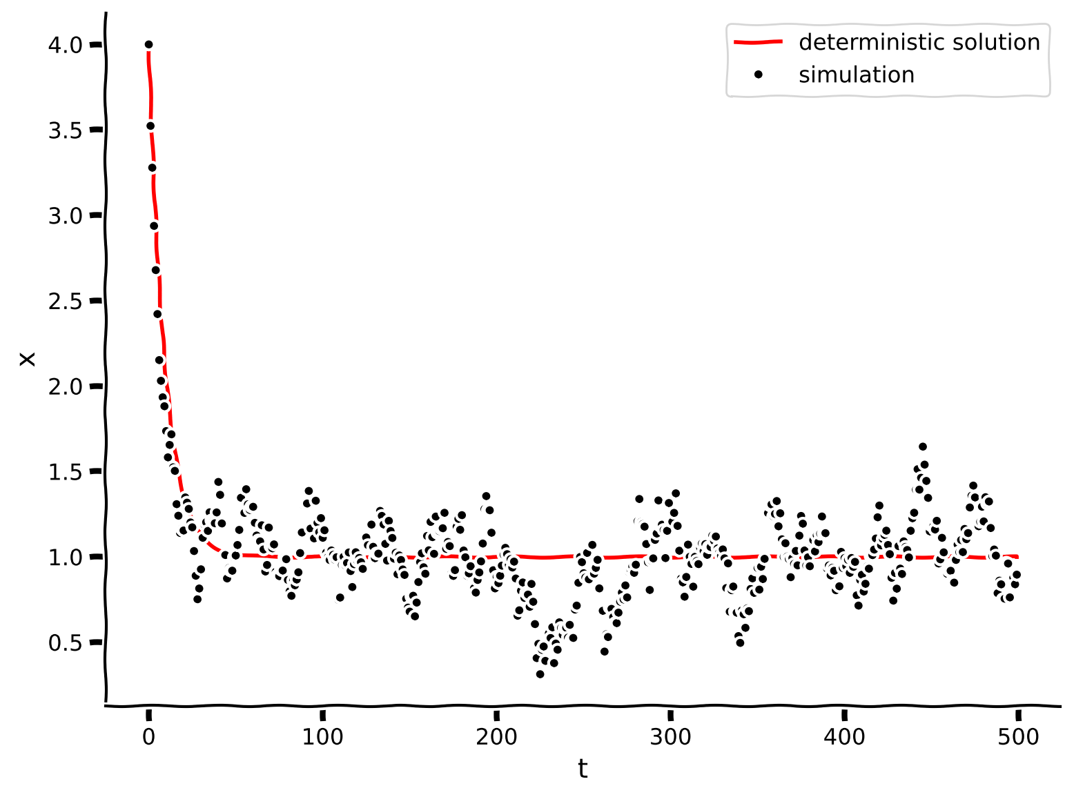
以下のコードを修正して、時間の各ステップに_決定論的_な部分(ヒント: 上のコードと全く同じ)と、標準偏差 (コード内では sig)を持つ正規分布から引かれる_ランダムで拡散的_な部分を加えてください。この過程の動態をプロットします。
def simulate_ddm(lam, sig, x0, xinfty, T):
  """
  Simulate the drift-diffusion model with given parameters and initial condition.
  Args:
    lam (scalar): decay rate
    sig (scalar): standard deviation of normal distribution
    x0 (scalar): initial condition (x at time 0)
    xinfty (scalar): drift towards convergence in the limit
    T (scalar): total duration of the simulation (in steps)

  Returns:
    ndarray, ndarray: `x` for all simulation steps and the time `t` at each step
  """

  # initialize variables
  t = np.arange(0, T, 1.)
  x = np.zeros_like(t)
  x[0] = x0

  # Step through in time
  for k in range(len(t)-1):
    ##############################################################################
    ## TODO: Insert your code below then remove
    raise NotImplementedError("Student exercise: need to implement simulation")
    ##############################################################################
    # update x at time k+1 with a deterministic and a stochastic component
    # hint: the deterministic component will be like above, and
    #   the stochastic component is drawn from a scaled normal distribution
    x[k+1] = ...

  return t, x


lam = 0.9  # decay rate
sig = 0.1  # standard deviation of diffusive process
T = 500  # total Time duration in steps
x0 = 4.  # initial condition of x at time 0
xinfty = 1.  # x drifts towards this value in long time

# Plot x as it evolves in time
np.random.seed(2020)
t, x = simulate_ddm(lam, sig, x0, xinfty, T)
plot_ddm(t, x, xinfty, lam, x0)出力例:
# @title Submit your feedback
content_review(f"{feedback_prefix}_DriftDiffusion_model_Exercise")
考えてみよう!2: ドリフト-拡散シミュレーションの観察
シミュレーションの振る舞いを観察して説明してください。決定論的解と比べてどうですか?刺激の初めと終わりでどのように振る舞いますか?
# @title Submit your feedback
content_review(f"{feedback_prefix}_DriftDiffusion_Simulation_Observations_Discussion")
セクション3: OU過程の分散
チュートリアル開始からここまでの推定所要時間: 35分
# @title Video 3: Balance of Variances
from ipywidgets import widgets
from IPython.display import YouTubeVideo
from IPython.display import IFrame
from IPython.display import display


class PlayVideo(IFrame):
  def __init__(self, id, source, page=1, width=400, height=300, **kwargs):
    self.id = id
    if source == 'Bilibili':
      src = f'https://player.bilibili.com/player.html?bvid={id}&page={page}'
    elif source == 'Osf':
      src = f'https://mfr.ca-1.osf.io/render?url=https://osf.io/download/{id}/?direct%26mode=render'
    super(PlayVideo, self).__init__(src, width, height, **kwargs)


def display_videos(video_ids, W=400, H=300, fs=1):
  tab_contents = []
  for i, video_id in enumerate(video_ids):
    out = widgets.Output()
    with out:
      if video_ids[i][0] == 'Youtube':
        video = YouTubeVideo(id=video_ids[i][1], width=W,
                             height=H, fs=fs, rel=0)
        print(f'Video available at https://youtube.com/watch?v={video.id}')
      else:
        video = PlayVideo(id=video_ids[i][1], source=video_ids[i][0], width=W,
                          height=H, fs=fs, autoplay=False)
        if video_ids[i][0] == 'Bilibili':
          print(f'Video available at https://www.bilibili.com/video/{video.id}')
        elif video_ids[i][0] == 'Osf':
          print(f'Video available at https://osf.io/{video.id}')
      display(video)
    tab_contents.append(out)
  return tab_contents


video_ids = [('Youtube', '49A-3kftau0'), ('Bilibili', 'BV15f4y1R7PU')]
tab_contents = display_videos(video_ids, W=854, H=480)
tabs = widgets.Tab()
tabs.children = tab_contents
for i in range(len(tab_contents)):
  tabs.set_title(i, video_ids[i][0])
display(tabs)
# @title Submit your feedback
content_review(f"{feedback_prefix}_Balance_of_Variances_Video")ご覧の通り、過程の平均は支配方程式の決定論的部分の解に従います。ここまでは順調です!
では、分散はどうでしょう?
ランダムウォークとは異なり、 を に「引き戻す」減衰過程があるため、分散は時間が大きくなっても無限に増加しません。代わりに、 から遠ざかると位置が戻され、平衡状態に達します。
このドリフト-拡散システムの平衡分散は
この平衡分散の値は と に依存し、 や には依存しません。
動作が妥当であることを確かめるために、OU方程式の平衡解の経験的分散と理論式を比較してみましょう。
コーディング演習3: 経験的分散の計算
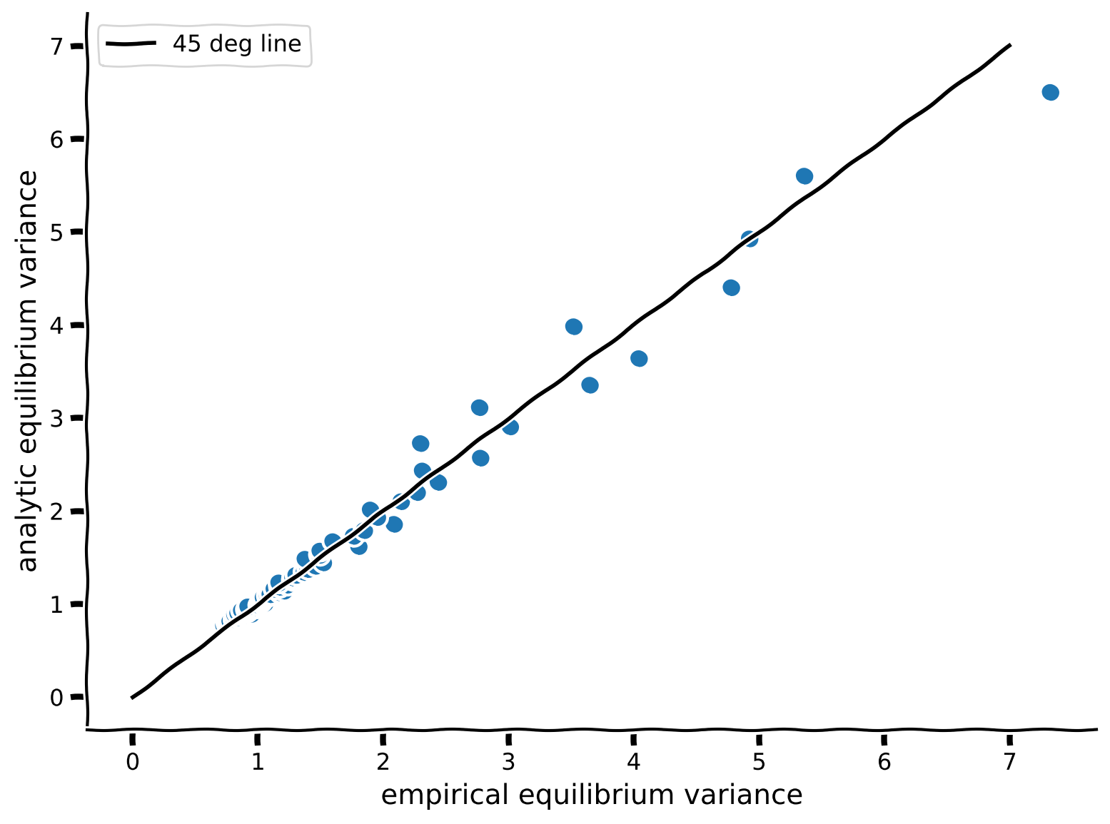
解析的分散 を計算し、経験的分散(ヘルパー関数で既に提供されています)と比較するコードを書いてください。両者はほぼ等しく、45度線()の近くに並ぶはずです。
def ddm(T, x0, xinfty, lam, sig):
  t = np.arange(0, T, 1.)
  x = np.zeros_like(t)
  x[0] = x0

  for k in range(len(t)-1):
    x[k+1] = xinfty + lam * (x[k] - xinfty) + sig * np.random.standard_normal(size=1)

  return t, x


# computes equilibrium variance of ddm
# returns variance
def ddm_eq_var(T, x0, xinfty, lam, sig):
  t, x = ddm(T, x0, xinfty, lam, sig)

  # returns variance of the second half of the simulation
  # this is a hack: assumes system has settled by second half
  return x[-round(T/2):].var()


np.random.seed(2020) # set random seed

# sweep through values for lambda
lambdas = np.arange(0.05, 0.95, 0.01)
empirical_variances = np.zeros_like(lambdas)
analytical_variances = np.zeros_like(lambdas)

sig = 0.87

# compute empirical equilibrium variance
for i, lam in enumerate(lambdas):
  empirical_variances[i] = ddm_eq_var(5000, x0, xinfty, lambdas[i], sig)

##############################################################################
## Insert your code below to calculate the analytical variances
raise NotImplementedError("Student exercise: need to compute variances")
##############################################################################

# Hint: you can also do this in one line outside the loop!
analytical_variances = ...

# Plot the empirical variance vs analytical variance
var_comparison_plot(empirical_variances, analytical_variances)出力例:
# @title Submit your feedback
content_review(f"{feedback_prefix}_Computing_the_variances_empirically_Exercise")
まとめ
チュートリアルの推定所要時間: 45分
このチュートリアルでは、決定論的部分と確率的部分の両方を持つOUシステムを構築し観察しました。平均的には決定論的力学系の解析から期待される振る舞いに似ていることがわかりました。
重要なのは、決定論的部分と確率的部分の相互作用が、純粋に確率的な過程(ランダムウォークのように)で時間とともに分散が増加する傾向を_バランス_させることです。この振る舞いは、短期記憶や意思決定を含む認知機能のモデル化にOUシステムが好まれる理由の一つです。