チュートリアル 2: マルコフ過程

第2週、第3日目：線形システム

Neuromatch Academy 提供

コンテンツ作成者: Bing Wen Brunton, Ellie Stradquist

コンテンツレビュアー: Norma Kuhn, Karolina Stosio, John Butler, Matthew Krause, Ella Batty, Richard Gao, Michael Waskom, Ethan Cheng

制作編集者: Gagana B, Spiros Chavlis

チュートリアルの目的

チュートリアルの推定所要時間：45分

このチュートリアルでは、最初のチュートリアルで紹介した動的システムを別の視点から見ていきます。

チュートリアル1では、動的システムを決定論的プロセスとして学びました。チュートリアル2では、確率的動的システムを扱います。これらのシステムは時に_確率過程_（stochastic）とも呼ばれます。確率的プロセスでは、ランダム性の要素が含まれます。同じ初期条件から観察しても、結果は毎回異なる可能性があります。言い換えれば、確率を含む動的システムは、その振る舞いにランダムな変動を取り入れています。

一部の確率的動的システムでは、微分方程式が時刻 $t$ における $\dot{x}$ と $x$ の関係を表し、_すべての_時刻における $x$ の方向が $x$ の値のみに完全に依存します。別の言い方をすると、時刻 $t$ における状態変数 $x$ の値を知ることが、$\dot{x}$ を決定し、次の時刻の $x$ を決めるために必要な_すべて_の情報となります。

この性質――現在の状態が次の状態への遷移を完全に決定する――がマルコフ過程の定義であり、この性質を満たすシステムはマルコフ性を持つと言えます。

チュートリアル2の目的は、このタイプのマルコフ過程を、状態遷移が確率的である単純な例で考察することです。具体的には：

• マルコフ過程と履歴依存性を理解する。
• 2状態のテレグラフ過程の振る舞いを調べ、その平衡分布がパラメータに依存する様子を理解する。

# @title Tutorial slides
# @markdown These are the slides for the videos in all tutorials today
from IPython.display import IFrame
link_id = "snv4m"
print(f"If you want to download the slides: https://osf.io/download/{link_id}/")
IFrame(src=f"https://mfr.ca-1.osf.io/render?url=https://osf.io/{link_id}/?direct%26mode=render%26action=download%26mode=render", width=854, height=480)

セットアップ

# @title Install and import feedback gadget


from vibecheck import DatatopsContentReviewContainer
def content_review(notebook_section: str):
    return DatatopsContentReviewContainer(
        "",  # No text prompt
        notebook_section,
        {
            "url": "https://pmyvdlilci.execute-api.us-east-1.amazonaws.com/klab",
            "name": "neuromatch_cn",
            "user_key": "y1x3mpx5",
        },
    ).render()


feedback_prefix = "W2D2_T2"

# Imports
import numpy as np
import matplotlib.pyplot as plt

# @title Figure Settings
import logging
logging.getLogger('matplotlib.font_manager').disabled = True
import ipywidgets as widgets  # interactive display
%config InlineBackend.figure_format = 'retina'
plt.style.use("https://raw.githubusercontent.com/NeuromatchAcademy/course-content/main/nma.mplstyle")

# @title Plotting Functions

def plot_switch_simulation(t, x):
  plt.figure()
  plt.plot(t, x)
  plt.title('State-switch simulation')
  plt.xlabel('Time')
  plt.xlim((0, 300)) # zoom in time
  plt.ylabel('State of ion channel 0/1', labelpad=-60)
  plt.yticks([0, 1], ['Closed (0)', 'Open (1)'])
  plt.show()


def plot_interswitch_interval_histogram(inter_switch_intervals):
  plt.figure()
  plt.hist(inter_switch_intervals)
  plt.title('Inter-switch Intervals Distribution')
  plt.ylabel('Interval Count')
  plt.xlabel('time')
  plt.show()


def plot_state_probabilities(time, states):
  plt.figure()
  plt.plot(time, states[:, 0], label='Closed')
  plt.plot(time, states[:, 1], label='Open')
  plt.xlabel('time')
  plt.ylabel('prob(open OR closed)')
  plt.legend()
  plt.show()

セクション1: テレグラフ過程

# @title Video 1: Markov Process
from ipywidgets import widgets
from IPython.display import YouTubeVideo
from IPython.display import IFrame
from IPython.display import display


class PlayVideo(IFrame):
  def __init__(self, id, source, page=1, width=400, height=300, **kwargs):
    self.id = id
    if source == 'Bilibili':
      src = f'https://player.bilibili.com/player.html?bvid={id}&page={page}'
    elif source == 'Osf':
      src = f'https://mfr.ca-1.osf.io/render?url=https://osf.io/download/{id}/?direct%26mode=render'
    super(PlayVideo, self).__init__(src, width, height, **kwargs)


def display_videos(video_ids, W=400, H=300, fs=1):
  tab_contents = []
  for i, video_id in enumerate(video_ids):
    out = widgets.Output()
    with out:
      if video_ids[i][0] == 'Youtube':
        video = YouTubeVideo(id=video_ids[i][1], width=W,
                             height=H, fs=fs, rel=0)
        print(f'Video available at https://youtube.com/watch?v={video.id}')
      else:
        video = PlayVideo(id=video_ids[i][1], source=video_ids[i][0], width=W,
                          height=H, fs=fs, autoplay=False)
        if video_ids[i][0] == 'Bilibili':
          print(f'Video available at https://www.bilibili.com/video/{video.id}')
        elif video_ids[i][0] == 'Osf':
          print(f'Video available at https://osf.io/{video.id}')
      display(video)
    tab_contents.append(out)
  return tab_contents


video_ids = [('Youtube', 'xZO6GbU48ns'), ('Bilibili', 'BV11C4y1h7Eu')]
tab_contents = display_videos(video_ids, W=854, H=480)
tabs = widgets.Tab()
tabs.children = tab_contents
for i in range(len(tab_contents)):
  tabs.set_title(i, video_ids[i][0])
display(tabs)

# @title Submit your feedback
content_review(f"{feedback_prefix}_Markov_Process_Video")

このビデオでは、マルコフ過程の定義と、テレグラフ過程の例としてイオンチャネルの開閉について紹介します。

2つの状態を持ち、それぞれの状態間の切り替えが確率的であるマルコフ過程（テレグラフ過程）を考えましょう。具体的には、ニューロンのイオンチャネルが2つの状態のいずれかにあるとモデル化します：閉じている（0）か開いている（1）か。

イオンチャネルが閉じている場合、状態が開く状態に遷移する確率は $P(0 \rightarrow 1 | x = 0) = \mu_{c2o}$ です。同様に、イオンチャネルが開いている場合、閉じる状態に遷移する確率は $P(1 \rightarrow 0 | x=1) = \mu_{o2c}$ です。

状態変化の過程はポアソン過程としてシミュレートします。ポアソン過程は前提統計学の日$で学びました。ポアソン過程は、イベント間の平均時間が既知であるが、特定のイベントの正確な発生時間は不明な離散イベントをモデル化する方法です。重要な点は以下の通りです：

1. あるイベントが起こる確率は、他のすべてのイベントから独立している。
2. 一定期間内のイベントの平均発生率は一定である。
3. 同時に2つのイベントは発生しない。イオンチャネルは開いているか閉じているかのどちらかであり、同時に両方ではない。

以下のシミュレーションでは、ポアソン過程を用いて、総シミュレーション時間 $T$ のすべての時点 $t$ におけるイオンチャネルの状態をモデル化します。

状態変化のシミュレーションを行う際、状態が切り替わった時刻も追跡します。これらの時刻を使って、状態切り替え間の時間_間隔_の分布を測定できます。

マルコフ過程は前提統計学の日でも簡単に触れました。

以下のセルを実行すると状態変化のシミュレーション過程が表示されます。コード内で乱数シードが設定されているため、再実行しても同じプロットが得られます。この行をコメントアウトすると、実行ごとに異なるシミュレーション結果が得られます。

# @markdown Execute to simulate and plot state changes

# parameters
T = 5000     # total Time duration
dt = 0.001   # timestep of our simulation

# simulate state of our ion channel in time
# the two parameters that govern transitions are
# c2o: closed to open rate
# o2c: open to closed rate
def ion_channel_opening(c2o, o2c, T, dt):
  # initialize variables
  t = np.arange(0, T, dt)
  x = np.zeros_like(t)
  switch_times = []

  # assume we always start in Closed state
  x[0] = 0

  # generate a bunch of random uniformly distributed numbers
  # between zero and unity: [0, 1),
  # one for each dt in our simulation.
  # we will use these random numbers to model the
  # closed/open transitions
  myrand = np.random.random_sample(size=len(t))


  # walk through time steps of the simulation
  for k in range(len(t)-1):
    # switching between closed/open states are
    # Poisson processes
    if x[k] == 0 and myrand[k] < c2o*dt: # remember to scale by dt!
      x[k+1:] = 1
      switch_times.append(k*dt)
    elif x[k] == 1 and myrand[k] < o2c*dt:
      x[k+1:] = 0
      switch_times.append(k*dt)

  return t, x, switch_times


c2o = 0.02
o2c = 0.1
np.random.seed(0) # set random seed
t, x, switch_times = ion_channel_opening(c2o, o2c, T, .1)
plot_switch_simulation(t, x)

コーディング演習1: 状態切り替え間隔の計算

ビデオ中では演習2Aとして言及されています

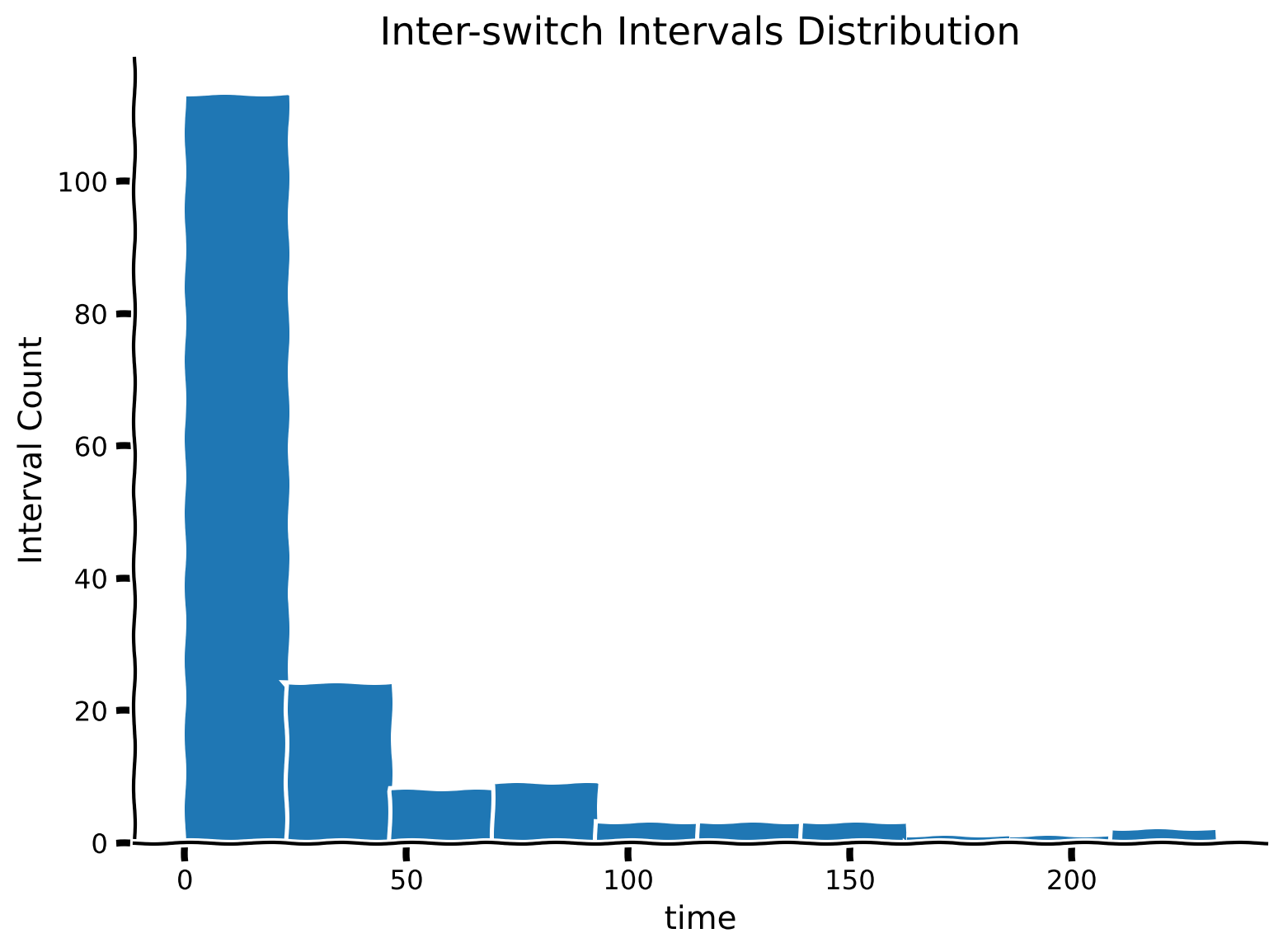
switch_times は状態が切り替わった時刻のリストです。これを使って、各状態切り替え間の時間間隔を計算し、inter_switch_intervals というリストに格納してください。

その後、これらの間隔の分布をプロットします。分布の形状をどのように説明しますか？

##############################################################################
## TODO: Insert your code here to calculate between-state-switch intervals
raise NotImplementedError("Student exercise: need to calculate switch intervals")
##############################################################################

# hint: see np.diff()
inter_switch_intervals = ...

# plot inter-switch intervals
plot_interswitch_interval_histogram(inter_switch_intervals)

解答を見る$

出力例:

# @title Submit your feedback
content_review(f"{feedback_prefix}_Computing_intervals_between_switches_Exercises")

次のセルでは、シミュレーション中にシステムが2つの可能な状態のいずれかに滞在した時間ステップ数の分布を棒グラフで可視化します。

# @markdown Execute cell to visualize distribution of time spent in each state.

states = ['Closed', 'Open']
(unique, counts) = np.unique(x, return_counts=True)

plt.figure()
plt.bar(states, counts)
plt.ylabel('Number of time steps')
plt.xlabel('State of ion channel')
plt.show()

状態は_離散的_であり、イオンチャネルは閉じているか開いているかのどちらかですが、システムの平均状態を一定時間のウィンドウで平均して見ることができます。

閉じている状態を $x=0$、開いている状態を $x=1$ とコード化しているため、$x$ の平均はチャネルが開いている時間の割合として解釈できます。

また、状態 $x$ の累積平均としての開いている割合も見てみましょう。累積平均は、ある時間経過後にシステムが経験した状態変化の平均回数を示します。

# @markdown Execute to visualize cumulative mean of state
plt.figure()
plt.plot(t, np.cumsum(x) / np.arange(1, len(t)+1))
plt.xlabel('time')
plt.ylabel('Cumulative mean of state')
plt.show()

上のプロットでは、チャネルは閉じた状態（$x=0$）から始まりましたが、時間が経つにつれてある平均値に収束していることがわかります。この平均値は遷移確率 $\mu_{c2o}$ と
$\mu_{o2c}$ に関連しています。

インタラクティブデモ1: 遷移確率値と $T$ の変化

以下のインタラクティブデモを使って、状態遷移確率 $\mu_{c2o}$ と $\mu_{o2c}$ の異なる値で状態切り替えシミュレーションを試してください。また、総シミュレーション時間 $T$ の値も変えてみてください。

1. 状態切り替え間隔の分布の全体的な形は変わりますか、それともほぼ同じままですか？
2. システム状態の棒グラフはこれらの値によってどのように変化しますか？

# @markdown Make sure you execute this cell to enable the widget!

@widgets.interact
def plot_inter_switch_intervals(c2o=(0,1, .01), o2c=(0, 1, .01),
                                T=(1000, 10000, 1000)):

  t, x, switch_times = ion_channel_opening(c2o, o2c, T, .1)

  inter_switch_intervals = np.diff(switch_times)

  # plot inter-switch intervals
  plt.hist(inter_switch_intervals)
  plt.title('Inter-switch Intervals Distribution')
  plt.ylabel('Interval Count')
  plt.xlabel('time')
  plt.show()

解答を見る$

# @title Submit your feedback
content_review(f"{feedback_prefix}_Varying_transition_probability_values_and_T_Interactive_Demo_and_Discussion")

セクション2: 分布的視点

チュートリアル開始からここまでの推定所要時間：18分

# @title Video 2: State Transitions
from ipywidgets import widgets
from IPython.display import YouTubeVideo
from IPython.display import IFrame
from IPython.display import display


class PlayVideo(IFrame):
  def __init__(self, id, source, page=1, width=400, height=300, **kwargs):
    self.id = id
    if source == 'Bilibili':
      src = f'https://player.bilibili.com/player.html?bvid={id}&page={page}'
    elif source == 'Osf':
      src = f'https://mfr.ca-1.osf.io/render?url=https://osf.io/download/{id}/?direct%26mode=render'
    super(PlayVideo, self).__init__(src, width, height, **kwargs)


def display_videos(video_ids, W=400, H=300, fs=1):
  tab_contents = []
  for i, video_id in enumerate(video_ids):
    out = widgets.Output()
    with out:
      if video_ids[i][0] == 'Youtube':
        video = YouTubeVideo(id=video_ids[i][1], width=W,
                             height=H, fs=fs, rel=0)
        print(f'Video available at https://youtube.com/watch?v={video.id}')
      else:
        video = PlayVideo(id=video_ids[i][1], source=video_ids[i][0], width=W,
                          height=H, fs=fs, autoplay=False)
        if video_ids[i][0] == 'Bilibili':
          print(f'Video available at https://www.bilibili.com/video/{video.id}')
        elif video_ids[i][0] == 'Osf':
          print(f'Video available at https://osf.io/{video.id}')
      display(video)
    tab_contents.append(out)
  return tab_contents


video_ids = [('Youtube', 'U6YRhLuRhHg'), ('Bilibili', 'BV1uk4y1B7ru')]
tab_contents = display_videos(video_ids, W=854, H=480)
tabs = widgets.Tab()
tabs.children = tab_contents
for i in range(len(tab_contents)):
  tabs.set_title(i, video_ids[i][0])
display(tabs)

このビデオでは、イオンチャネルの開閉というテレグラフ過程を、確率的状態遷移の行列・ベクトル表現という別の形式で紹介します。

注意 このシステムは離散時間ステップで書かれており、$\mathbf{A}$ はステップ $k$ から $k+1$ への状態遷移を表します。これは上記の演習で行った、$\mathbf{A}$ が状態から状態の時間微分への関数を表すものとは異なります。

コーディング演習2: 確率の伝播

ビデオ中では演習2Bとして言及されています

以下のコードを完成させて、イオンチャネルの閉じる/開く確率の時間伝播をシミュレートしてください。変数 $x_kp1$（$k$ 時刻の $x$ プラス1の略）はループ内の各ステップ k で計算されるべきです。ただし、プロットするのは $x$ です。

def simulate_prob_prop(A, x0, dt, T):
  """ Simulate the propagation of probabilities given the transition matrix A,
  with initial state x0, for a duration of T at timestep dt.

  Args:
    A (ndarray): state transition matrix
    x0 (ndarray): state probabilities at time 0
    dt (scalar): timestep of the simulation
    T (scalar): total duration of the simulation

  Returns:
    ndarray, ndarray: `x` for all simulation steps and the time `t` at each step
  """

  # Initialize variables
  t = np.arange(0, T, dt)
  x = x0 # x at time t_0

  # Step through the system in time
  for k in range(len(t)-1):
    ###################################################################
    ## TODO: Insert your code here to compute x_kp1 (x at k plus 1)
    raise NotImplementedError("Student exercise: need to implement simulation")
    ## hint: use np.dot(a, b) function to compute the dot product
    ##       of the transition matrix A and the last state in x
    ## hint 2: use np.vstack to append the latest state to x
    ###################################################################

    # Compute the state of x at time k+1
    x_kp1 = ...

    # Stack (append) this new state onto x to keep track of x through time steps
    x = ...

  return x, t


# Set parameters
T = 500     # total Time duration
dt = 0.1   # timestep of our simulation

# same parameters as above
# c: closed rate
# o: open rate
c = 0.02
o = 0.1
A = np.array([[1 - c*dt, o*dt],
              [c*dt,     1 - o*dt]])

# Initial condition: start as Closed
x0 = np.array([[1, 0]])

# Simulate probabilities propagation
x, t = simulate_prob_prop(A, x0, dt, T)

# Visualize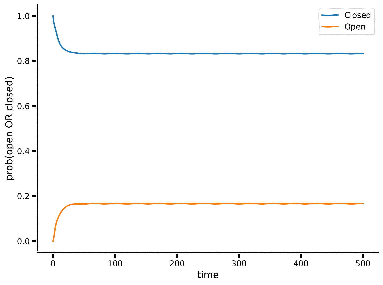
plot_state_probabilities(t, x)

解答を見る$

出力例:

# @title Submit your feedback
content_review(f"{feedback_prefix}_Probability_propagation_Exercise")

ここでは、イオンチャネルの状態変化の確率伝播を時間を通じてシミュレートしました。この方法の利点は、シミュレーションを1回実行するだけで、確率が時間を通じてどのように伝播するかを確認できることです。テレグラフ過程のシミュレーションを何度も繰り返して経験的に観察する必要がありません。

システムは初期に閉じた状態（$x=0$）から始まりましたが、時間が経つにつれて、$\mu$ パラメータの関数として開いている時間の割合を予測できる平衡分布に落ち着きます。上のプロットはこの_平衡への緩和_を示しています。

この方法で $c2o$ の確率を再計算すると、テレグラフ過程のシミュレーション結果と一致することがわかります。

print(f"Probability of state c2o: {(c2o / (c2o + o2c)):.3f}")

セクション3: テレグラフ過程の平衡状態

チュートリアル開始からここまでの推定所要時間：30分

# @title Video 3: Continuous vs. Discrete Time Formulation
from ipywidgets import widgets
from IPython.display import YouTubeVideo
from IPython.display import IFrame
from IPython.display import display


class PlayVideo(IFrame):
  def __init__(self, id, source, page=1, width=400, height=300, **kwargs):
    self.id = id
    if source == 'Bilibili':
      src = f'https://player.bilibili.com/player.html?bvid={id}&page={page}'
    elif source == 'Osf':
      src = f'https://mfr.ca-1.osf.io/render?url=https://osf.io/download/{id}/?direct%26mode=render'
    super(PlayVideo, self).__init__(src, width, height, **kwargs)


def display_videos(video_ids, W=400, H=300, fs=1):
  tab_contents = []
  for i, video_id in enumerate(video_ids):
    out = widgets.Output()
    with out:
      if video_ids[i][0] == 'Youtube':
        video = YouTubeVideo(id=video_ids[i][1], width=W,
                             height=H, fs=fs, rel=0)
        print(f'Video available at https://youtube.com/watch?v={video.id}')
      else:
        video = PlayVideo(id=video_ids[i][1], source=video_ids[i][0], width=W,
                          height=H, fs=fs, autoplay=False)
        if video_ids[i][0] == 'Bilibili':
          print(f'Video available at https://www.bilibili.com/video/{video.id}')
        elif video_ids[i][0] == 'Osf':
          print(f'Video available at https://osf.io/{video.id}')
      display(video)
    tab_contents.append(out)
  return tab_contents


video_ids = [('Youtube', 'csetTTauIh8'), ('Bilibili', 'BV1di4y1g7Yc')]
tab_contents = display_videos(video_ids, W=854, H=480)
tabs = widgets.Tab()
tabs.children = tab_contents
for i in range(len(tab_contents)):
  tabs.set_title(i, video_ids[i][0])
display(tabs)

# @title Submit your feedback
content_review(f"{feedback_prefix}_Continuous_vs_Discrete_time_fromulation_Video")

セクション2で遷移行列 $\mathbf{A}$ による確率伝播をモデル化したので、$\mathbf{A}$ の固有分解とシステムの平衡状態の振る舞いを結びつけましょう。

講義ビデオで紹介したように、$\mathbf{A}$ の固有値はシステムの安定性、特に対応する固有ベクトルの方向に関する情報を与えます。

# compute the eigendecomposition of A
lam, v = np.linalg.eig(A)

# print the 2 eigenvalues
print(f"Eigenvalues: {lam}")

# print the 2 eigenvectors
eigenvector1 = v[:, 0]
eigenvector2 = v[:, 1]
print(f"Eigenvector 1: {eigenvector1}")
print(f"Eigenvector 2: {eigenvector2}")

考えてみよう3: 安定状態の発見

1. これらの固有値のうち、どれが安定（平衡）解に対応していますか？
2. その固有値の固有ベクトルは何ですか？
3. それはセクション2のシミュレーションにおける平衡解をどのように説明していますか？

ヒント: シミュレーションは確率で書かれているため、確率の和は1になります。したがって、固有ベクトルの要素も和が1になるようにスケールすると、シミュレーションの状態確率と直接比較できます。

解答を見る$

# @title Submit your feedback
content_review(f"{feedback_prefix}_Finding_a_stable_state_Discussion")

まとめ

チュートリアルの推定所要時間：45分

このチュートリアルで学んだこと：

• 履歴依存性を持つマルコフ過程の定義。
• 単純な2状態マルコフ過程――テレグラフ過程――の振る舞いは、状態変化のシミュレーションとしても確率分布の伝播としてもシミュレートできること。
• 連続時間または離散時間で表現される動的システムの安定性解析の関係。
• テレグラフ過程の平衡挙動は予測可能であり、チュートリアル1で学んだ決定論的システムと同様に、$\mathbf{A}$ 行列の固有分解を用いて理解できること。