チュートリアル 1: 線形力学系

第2週、第3日目：線形システム

Neuromatch Academyによる

コンテンツ作成者: Bing Wen Brunton, Alice Schwarze

コンテンツレビュアー: Norma Kuhn, Karolina Stosio, John Butler, Matthew Krause, Ella Batty, Richard Gao, Michael Waskom

制作編集者: Gagana B, Spiros Chavlis

チュートリアルの目標

チュートリアルの推定所要時間：1時間

このチュートリアルでは、時間とともに変化するシステム、すなわち時間発展のルールが微分方程式で正確に記述される動的システムの挙動について学びます。

微分方程式は状態変数 $x$ の変化率を表す方程式です。通常、微分方程式の左辺に時間に関する $x$ の微分（ $dx/dt$ ）を用いて変化率を表します：

\frac{dx}{dt} = f(x)

よく使われる記法として、 $\frac{dx}{dt}$ を $\dot{x}$ と書きます。点は「時間に関する微分」を意味します。

本日は、 $f(x)$ が $x$ の線形関数である線形力学に焦点を当てます。チュートリアル1では以下を行います：

$x$ が単一変数の場合のシステムの挙動を探索し理解する
状態ベクトル $\mathbf{x}$ が2つの変数を表す場合を考える

# @title Tutorial slides
# @markdown These are the slides for the videos in all tutorials today
from IPython.display import IFrame
link_id = "snv4m"
print(f"If you want to download the slides: https://osf.io/download/{link_id}/")
IFrame(src=f"https://mfr.ca-1.osf.io/render?url=https://osf.io/{link_id}/?direct%26mode=render%26action=download%26mode=render", width=854, height=480)

セットアップ

# @title Install and import feedback gadget


from vibecheck import DatatopsContentReviewContainer
def content_review(notebook_section: str):
    return DatatopsContentReviewContainer(
        "",  # No text prompt
        notebook_section,
        {
            "url": "https://pmyvdlilci.execute-api.us-east-1.amazonaws.com/klab",
            "name": "neuromatch_cn",
            "user_key": "y1x3mpx5",
        },
    ).render()


feedback_prefix = "W2D2_T1"

# Imports
import numpy as np
import matplotlib.pyplot as plt
from scipy.integrate import solve_ivp  # numerical integration solver

# @title Figure settings
import logging
logging.getLogger('matplotlib.font_manager').disabled = True

import ipywidgets as widgets  # interactive display
%config InlineBackend.figure_format = 'retina'
plt.style.use("https://raw.githubusercontent.com/NeuromatchAcademy/course-content/main/nma.mplstyle")

# @title Plotting Functions
def plot_trajectory(system, params, initial_condition, dt=0.1, T=6,
                    figtitle=None):

  """
  Shows the solution of a linear system with two variables in 3 plots.
  The first plot shows x1 over time. The second plot shows x2 over time.
  The third plot shows x1 and x2 in a phase portrait.

  Args:
    system (function): a function f(x) that computes a derivative from
                        inputs (t, [x1, x2], *params)
    params (list or tuple): list of parameters for function "system"
    initial_condition (list or array): initial condition x0
    dt (float): time step of simulation
    T (float): end time of simulation
    figtitlte (string): title for the figure

  Returns:
    nothing, but it shows a figure
  """

  # time points for which we want to evaluate solutions
  t = np.arange(0, T, dt)

  # Integrate
  # use built-in ode solver
  solution = solve_ivp(system,
                    t_span=(0, T),
                    y0=initial_condition, t_eval=t,
                    args=(params),
                    dense_output=True)
  x = solution.y

  # make a color map to visualize time
  timecolors = np.array([(1 , 0 , 0, i)  for i in t / t[-1]])

  # make a large figure
  fig, (ah1, ah2, ah3) = plt.subplots(1, 3)
  fig.set_size_inches(10, 3)

  # plot x1 as a function of time
  ah1.scatter(t, x[0,], color=timecolors)
  ah1.set_xlabel('time')
  ah1.set_ylabel('x1', labelpad=-5)

  # plot x2 as a function of time
  ah2.scatter(t, x[1], color=timecolors)
  ah2.set_xlabel('time')
  ah2.set_ylabel('x2', labelpad=-5)

  # plot x1 and x2 in a phase portrait
  ah3.scatter(x[0,], x[1,], color=timecolors)
  ah3.set_xlabel('x1')
  ah3.set_ylabel('x2', labelpad=-5)
  #include initial condition is a blue cross
  ah3.plot(x[0,0], x[1,0], 'bx')

  # adjust spacing between subplots
  plt.subplots_adjust(wspace=0.5)

  # add figure title
  if figtitle is not None:
    fig.suptitle(figtitle, size=16)
  plt.show()


def plot_streamplot(A, ax, figtitle=None, show=True):
  """
  Show a stream plot for a linear ordinary differential equation with
  state vector x=[x1,x2] in axis ax.

  Args:
    A (numpy array): 2x2 matrix specifying the dynamical system
    ax (matplotlib.axes): axis to plot
    figtitle (string): title for the figure
    show (boolean): enable plt.show()

  Returns:
    nothing, but shows a figure
  """

  # sample 20 x 20 grid uniformly to get x1 and x2
  grid = np.arange(-20, 21, 1)
  x1, x2 = np.meshgrid(grid, grid)

  # calculate x1dot and x2dot at each grid point
  x1dot = A[0,0] * x1 + A[0,1] * x2
  x2dot = A[1,0] * x1 + A[1,1] * x2

  # make a colormap
  magnitude = np.sqrt(x1dot ** 2 + x2dot ** 2)
  color = 2 * np.log1p(magnitude) #Avoid taking log of zero

  # plot
  plt.sca(ax)
  plt.streamplot(x1, x2, x1dot, x2dot, color=color,
                 linewidth=1, cmap=plt.cm.cividis,
                 density=2, arrowstyle='->', arrowsize=1.5)
  plt.xlabel(r'$x1$')
  plt.ylabel(r'$x2$')

  # figure title
  if figtitle is not None:
    plt.title(figtitle, size=16)

  # include eigenvectors
  if True:
    # get eigenvalues and eigenvectors of A
    lam, v = np.linalg.eig(A)

    # get eigenvectors of A
    eigenvector1 = v[:,0].real
    eigenvector2 = v[:,1].real

    # plot eigenvectors
    plt.arrow(0, 0, 20*eigenvector1[0], 20*eigenvector1[1],
              width=0.5, color='r', head_width=2,
              length_includes_head=True)
    plt.arrow(0, 0, 20*eigenvector2[0], 20*eigenvector2[1],
              width=0.5, color='b', head_width=2,
              length_includes_head=True)
  if show:
    plt.show()


def plot_specific_example_stream_plots(A_options):
  """
  Show a stream plot for each A in A_options

  Args:
    A (list): a list of numpy arrays (each element is A)

  Returns:
    nothing, but shows a figure
  """
  # get stream plots for the four different systems
  plt.figure(figsize=(10, 10))

  for i, A in enumerate(A_options):

    ax = plt.subplot(2, 2, 1+i)
    # get eigenvalues and eigenvectors
    lam, v = np.linalg.eig(A)

    # plot eigenvalues as title
    # (two spaces looks better than one)
    eigstr = ",  ".join([f"{x:.2f}" for x in lam])
    figtitle =f"A with eigenvalues\n"+ '[' + eigstr + ']'
    plot_streamplot(A, ax, figtitle=figtitle, show=False)

    # Remove y_labels on righthand plots
    if i % 2:
      ax.set_ylabel(None)
    if i < 2:
      ax.set_xlabel(None)

    plt.subplots_adjust(wspace=0.3, hspace=0.3)
  plt.show()

セクション1：1次元微分方程式

# @title Video 1: Linear Dynamical Systems
from ipywidgets import widgets
from IPython.display import YouTubeVideo
from IPython.display import IFrame
from IPython.display import display


class PlayVideo(IFrame):
  def __init__(self, id, source, page=1, width=400, height=300, **kwargs):
    self.id = id
    if source == 'Bilibili':
      src = f'https://player.bilibili.com/player.html?bvid={id}&page={page}'
    elif source == 'Osf':
      src = f'https://mfr.ca-1.osf.io/render?url=https://osf.io/download/{id}/?direct%26mode=render'
    super(PlayVideo, self).__init__(src, width, height, **kwargs)


def display_videos(video_ids, W=400, H=300, fs=1):
  tab_contents = []
  for i, video_id in enumerate(video_ids):
    out = widgets.Output()
    with out:
      if video_ids[i][0] == 'Youtube':
        video = YouTubeVideo(id=video_ids[i][1], width=W,
                             height=H, fs=fs, rel=0)
        print(f'Video available at https://youtube.com/watch?v={video.id}')
      else:
        video = PlayVideo(id=video_ids[i][1], source=video_ids[i][0], width=W,
                          height=H, fs=fs, autoplay=False)
        if video_ids[i][0] == 'Bilibili':
          print(f'Video available at https://www.bilibili.com/video/{video.id}')
        elif video_ids[i][0] == 'Osf':
          print(f'Video available at https://osf.io/{video.id}')
      display(video)
    tab_contents.append(out)
  return tab_contents


video_ids = [('Youtube', '87z6OR7-DBI'), ('Bilibili', 'BV1up4y1S7wj')]
tab_contents = display_videos(video_ids, W=854, H=480)
tabs = widgets.Tab()
tabs.children = tab_contents
for i in range(len(tab_contents)):
  tabs.set_title(i, video_ids[i][0])
display(tabs)

# @title Submit your feedback
content_review(f"{feedback_prefix}_Linear_Dynamical_Systems_Video")

このビデオは、時間とともに変化するものの数学としての動的システムの入門であり、神経科学に関連する時間スケールの例も含みます。線形システムの定義と、なぜ線形力学系に丸一日を費やすのかを説明し、1次元の決定論的動的システムの解法、その挙動、安定性基準を解説します。

なお、このセクションはプレコースの微積分デイのチュートリアル2 $と[3](https://compneuro.ne$ uromatch.io/tutorials/W0D4_Calculus/student/W0D4_Tutorial3.html)$の復習です。

ビデオのテキスト要約はこちらをクリック

まず、 $x$ に関する1次元微分方程式

\dot{x} = a x

を思い出しましょう。ここで $a$ はスカラーです。

この微分方程式に従うときの $x$ の時間発展の解は次の形を取ります：

x(t) = x_0\exp(a t)

ここで $x_0$ は初期条件、すなわち時刻0での $x$ の値です。

さらなる直感を得るために、簡単なシミュレーションでこのようなシステムの挙動を探りましょう。常微分方程式は、時間を離散的な時刻 $t_0, t_1, t_2, \dots$ として近似し、 $t_{i+1}=t_i+dt$ としてシミュレートできます。微分の定義から、短時間 $dt$ における小さな変化 $dx$ は次のように得られます：

\begin{eqnarray}
$\dot x$ &=& $\frac{dx}{dt}$ \
dx &=& $\dot x$ , dt
\end{eqnarray}

したがって、各時刻 $t_i$ における $x$ の値 $x(t_i)$ は、前の時刻 $t_{i-1}$ での値 $x(t_{i-1})$ と小さな変化 $dx=\dot x\,dt$ の和として計算されます：

x(t_i)=x(t_{i-1})+\dot x(t_{i-1}) dt

この非常に単純な積分法は前進オイラー積分と呼ばれ、 $dt$ が小さく常微分方程式が単純な場合にうまく機能します。ノイズが多い場合や $x$ が急激に大きく変化する場合（例えば興奮性ニューロンモデルなど）には問題が生じることがあります。その場合は積分法の選択に注意が必要です。しかし、今回の単純なシステムではこの方法で十分です！

コーディング演習1：前進オイラー積分

ビデオ中では演習1Bとして言及されています

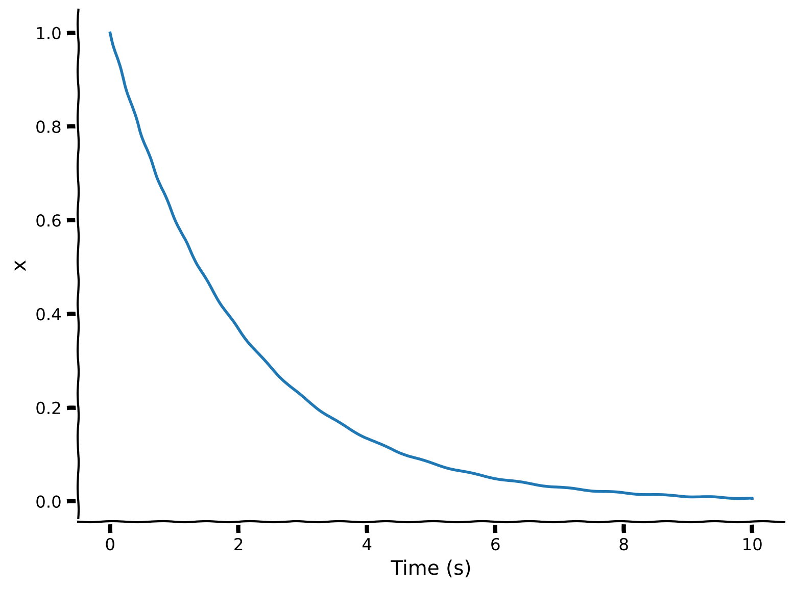
この演習では、微分方程式 $\dot{x} = a x$ の解を前進オイラー積分で計算する関数 integrate_exponential を完成させます。その後、時間に沿った解をプロットします。

def integrate_exponential(a, x0, dt, T):
  """Compute solution of the differential equation xdot=a*x with
  initial condition x0 for a duration T. Use time step dt for numerical
  solution.

  Args:
    a (scalar): parameter of xdot (xdot=a*x)
    x0 (scalar): initial condition (x at time 0)
    dt (scalar): timestep of the simulation
    T (scalar): total duration of the simulation

  Returns:
    ndarray, ndarray: `x` for all simulation steps and the time `t` at each step
  """

  # Initialize variables
  t = np.arange(0, T, dt)
  x = np.zeros_like(t, dtype=complex)
  x[0] = x0 # This is x at time t_0

  # Step through system and integrate in time
  for k in range(1, len(t)):

    ###################################################################
    ## Fill out the following then remove
    raise NotImplementedError("Student exercise: need to implement simulation")
    ###################################################################

    # for each point in time, compute xdot from x[k-1]
    xdot = ...

    # Update x based on x[k-1] and xdot
    x[k] = ...

  return x, t


# Choose parameters
a = -0.5    # parameter in f(x)
T = 10      # total Time duration
dt = 0.001  # timestep of our simulation
x0 = 1.     # initial condition of x at time 0

# Use Euler's method
x, t = integrate_exponential(a, x0, dt, T)

# Visualize
plt.plot(t, x.real)
plt.xlabel('Time (s)')
plt.ylabel('x')
plt.show()

解答を見る$

出力例:

# @title Submit your feedback
content_review(f"{feedback_prefix}_Forward_Euler_Integration_Exercise")

インタラクティブデモ1：前進オイラー積分

$a$ を変えるとどうなりますか？ $a<0$ と $a>0$ の値を試してみてください。
$dt$ は前進オイラー積分のステップサイズです。 $a = -1.5$ にして $dt$ を大きくすると数値解はどうなりますか？

# @markdown Make sure you execute this cell to enable the widget!

T = 10  # total Time duration
x0 = 1.  # initial condition of x at time 0

@widgets.interact(
    a=widgets.FloatSlider(value=-0.5, min=-2.5, max=1.5, step=0.25,
                          description="α", readout_format='.2f'),
    dt=widgets.FloatSlider(value=0.001, min=0.001, max=1.0, step=0.001,
                           description="dt", readout_format='.3f')
    )

def plot_euler_integration(a, dt):
  # Have to do this clunky word around to show small values in slider accurately
  # (from https://github.com/jupyter-widgets/ipywidgets/issues/259)

  x, t = integrate_exponential(a, x0, dt, T)
  plt.plot(t, x.real)  # integrate_exponential returns complex
  plt.xlabel('Time (s)')
  plt.ylabel('x')
  plt.show()

解答を見る$

# @title Submit your feedback
content_review(f"{feedback_prefix}_What_models_Video")

セクション2：振動動力学

チュートリアル開始からの推定所要時間：20分

# @title Video 2: Oscillatory Solutions
from ipywidgets import widgets
from IPython.display import YouTubeVideo
from IPython.display import IFrame
from IPython.display import display


class PlayVideo(IFrame):
  def __init__(self, id, source, page=1, width=400, height=300, **kwargs):
    self.id = id
    if source == 'Bilibili':
      src = f'https://player.bilibili.com/player.html?bvid={id}&page={page}'
    elif source == 'Osf':
      src = f'https://mfr.ca-1.osf.io/render?url=https://osf.io/download/{id}/?direct%26mode=render'
    super(PlayVideo, self).__init__(src, width, height, **kwargs)


def display_videos(video_ids, W=400, H=300, fs=1):
  tab_contents = []
  for i, video_id in enumerate(video_ids):
    out = widgets.Output()
    with out:
      if video_ids[i][0] == 'Youtube':
        video = YouTubeVideo(id=video_ids[i][1], width=W,
                             height=H, fs=fs, rel=0)
        print(f'Video available at https://youtube.com/watch?v={video.id}')
      else:
        video = PlayVideo(id=video_ids[i][1], source=video_ids[i][0], width=W,
                          height=H, fs=fs, autoplay=False)
        if video_ids[i][0] == 'Bilibili':
          print(f'Video available at https://www.bilibili.com/video/{video.id}')
        elif video_ids[i][0] == 'Osf':
          print(f'Video available at https://osf.io/{video.id}')
      display(video)
    tab_contents.append(out)
  return tab_contents


video_ids = [('Youtube', 'vPYQPI4nKT8'), ('Bilibili', 'BV1gZ4y1u7PK')]
tab_contents = display_videos(video_ids, W=854, H=480)
tabs = widgets.Tab()
tabs.children = tab_contents
for i in range(len(tab_contents)):
  tabs.set_title(i, video_ids[i][0])
display(tabs)

# @title Submit your feedback
content_review(f"{feedback_prefix}_Forward_Euler_Integration_Interactive_Demo_Discussion")

次に、 $a$ が複素数で虚数成分がゼロでない場合に何が起こるかを探ります。

インタラクティブデモ2：振動動力学

ビデオ中では演習1Bとして言及されています

以下のデモでは、 $a$ の実部と虚部（つまり $a = ext{実部} + ext{虚部} imes i$ ）を変更できます。

どのような $a$ の値が振動しつつ増大する動力学を生み出しますか？
0.5ヘルツ（周期/時間単位）の安定した振動を生み出すにはどのような $a$ の値が必要ですか？

# @markdown Make sure you execute this cell to enable the widget!

# parameters
T = 5  # total Time duration
dt = 0.0001  # timestep of our simulation
x0 = 1.  # initial condition of x at time 0

@widgets.interact
def plot_euler_integration(real=(-2, 2, .2), imaginary=(-4, 7, .1)):

  a = complex(real, imaginary)
  x, t = integrate_exponential(a, x0, dt, T)
  plt.plot(t, x.real)  # integrate exponential returns complex
  plt.grid(True)
  plt.xlabel('Time (s)')
  plt.ylabel('x')
  plt.show()

解答を見る$

# @title Submit your feedback
content_review(f"{feedback_prefix}_Oscillatory_Dynamics_Interactive_Demo_Discussion")

セクション3：2次元の決定論的線形力学系

チュートリアル開始からの推定所要時間：33分

# @title Video 3: Multi-Dimensional Dynamics
from ipywidgets import widgets
from IPython.display import YouTubeVideo
from IPython.display import IFrame
from IPython.display import display


class PlayVideo(IFrame):
  def __init__(self, id, source, page=1, width=400, height=300, **kwargs):
    self.id = id
    if source == 'Bilibili':
      src = f'https://player.bilibili.com/player.html?bvid={id}&page={page}'
    elif source == 'Osf':
      src = f'https://mfr.ca-1.osf.io/render?url=https://osf.io/download/{id}/?direct%26mode=render'
    super(PlayVideo, self).__init__(src, width, height, **kwargs)


def display_videos(video_ids, W=400, H=300, fs=1):
  tab_contents = []
  for i, video_id in enumerate(video_ids):
    out = widgets.Output()
    with out:
      if video_ids[i][0] == 'Youtube':
        video = YouTubeVideo(id=video_ids[i][1], width=W,
                             height=H, fs=fs, rel=0)
        print(f'Video available at https://youtube.com/watch?v={video.id}')
      else:
        video = PlayVideo(id=video_ids[i][1], source=video_ids[i][0], width=W,
                          height=H, fs=fs, autoplay=False)
        if video_ids[i][0] == 'Bilibili':
          print(f'Video available at https://www.bilibili.com/video/{video.id}')
        elif video_ids[i][0] == 'Osf':
          print(f'Video available at https://osf.io/{video.id}')
      display(video)
    tab_contents.append(out)
  return tab_contents


video_ids = [('Youtube', 'c_GdNS3YH_M'), ('Bilibili', 'BV1pf4y1R7uy')]
tab_contents = display_videos(video_ids, W=854, H=480)
tabs = widgets.Tab()
tabs.children = tab_contents
for i in range(len(tab_contents)):
  tabs.set_title(i, video_ids[i][0])
display(tabs)

# @title Submit your feedback
content_review(f"{feedback_prefix}_MultiDimensional_Dynamics_Video")

このビデオは、ベクトル・行列方程式で表される2次元の決定論的動的システムの入門です。ストリームプロットの説明と、位相図を遷移行列 $A$ の固有値・固有ベクトルと結びつける方法を解説します。

ビデオの関連部分のテキスト要約はこちらをクリック

変数（または_次元_）を1つ追加すると、より多様な挙動が現れます。複数のニューロンなど複雑なシステムの動的挙動をモデル化する際に有用です。2つの線形常微分方程式でこのシステムを表せます：

\begin{eqnarray}
$\dot{x}_1$ &=& { $a}_{11}$ $x_1$ \
$\dot{x}_2$ &=& { $a}_{22}$ $x_2$ \
\end{eqnarray}

これまでは2つの変数（例：ニューロン）が独立していました。面白くするために相互作用項を加えます：

\begin{eqnarray}
$\dot{x}_1$ &=& { $a}_{11}$ $x_1$ + { $a}_{12}$ $x_2$ \
$\dot{x}_2$ &=& { $a}_{21}$ $x_1$ + { $a}_{22}$ $x_2$ \
\end{eqnarray}

この2つの方程式は1つの（ベクトル値の）線形常微分方程式として書けます：

\dot{\mathbf{x}} = \mathbf{A} \mathbf{x}

2次元システムでは、 $\mathbf{x}$ は2要素のベクトル（ $x_1$ と $x_2$ ）、 $\mathbf{A}$ は $2 \times 2$ 行列で、 $\mathbf{A}=\bigg[\begin{array} & a_{11} & a_{12} \\ a_{21} & a_{22} \end{array} \bigg]$ です。

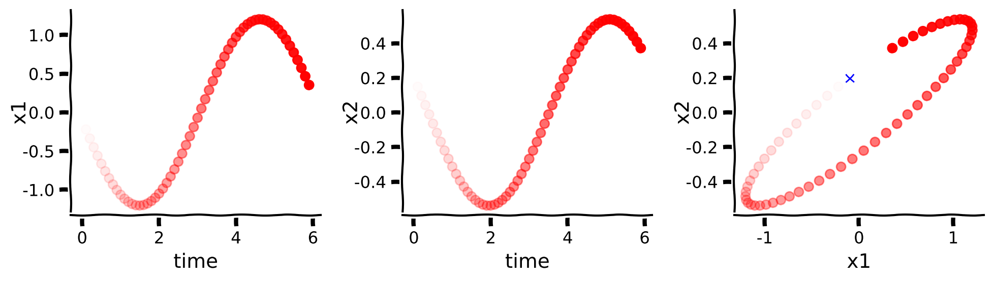
コーディング演習3：2次元の軌道サンプリング

ビデオ中では演習1Cのステップ1と2として言及されています

あるシステムの軌道をシミュレートし、 $x_1$ と $x_2$ が時間とともにどう変化するかをプロットします。例として以下のシステムを使います：

\dot{\mathbf{x}} = \bigg[\begin{array} & 2 & -5 \\ 1 & -2 \end{array} \bigg] \mathbf{x}

scipyの積分器を使うので自分で解く必要はありません。軌道をプロットするヘルパー関数 plot_trajectory があります。この演習では2変数の線形システムのシステム関数を作成します。

def system(t, x, a00, a01, a10, a11):
  '''
  Compute the derivative of the state x at time t for a linear
  differential equation with A matrix [[a00, a01], [a10, a11]].

  Args:
    t (float): time
    x (ndarray): state variable
    a00, a01, a10, a11 (float): parameters of the system

  Returns:
    ndarray: derivative xdot of state variable x at time t
  '''
  #################################################
  ## TODO for students: Compute xdot1 and xdot2 ##
  ## Fill out the following then remove
  raise NotImplementedError("Student exercise: say what they should have done")
  #################################################

  # compute x1dot and x2dot
  x1dot = ...
  x2dot = ...

  return np.array([x1dot, x2dot])


# Set parameters
T = 6 # total time duration
dt = 0.1 # timestep of our simulation
A = np.array([[2, -5],
              [1, -2]])
x0 = [-0.1, 0.2]

# Simulate and plot trajectories
plot_trajectory(system, [A[0, 0], A[0, 1], A[1, 0], A[1, 1]], x0, dt=dt, T=T)

解答を見る$

出力例:

# @title Submit your feedback
content_review(f"{feedback_prefix}_Sample_trajectories_in_2_dimensions_Exercise")

インタラクティブデモ3A：行列Aの変更

前の演習で作成した関数を使い、異なる行列 $A$ の軌道をプロットします。どのような質的に異なる動的挙動が観察されますか？

ヒント: x軸とy軸に注目してください！

# @markdown Make sure you execute this cell to enable the widget!

# parameters
T = 6  # total Time duration
dt = 0.1  # timestep of our simulation
x0 = np.asarray([-0.1, 0.2])  # initial condition of x at time 0

A_option_1 = [[2, -5],[1, -2]]
A_option_2 = [[3,4], [1, 2]]
A_option_3 = [[-1, -1], [0, -0.25]]
A_option_4 = [[3, -2],[2, -2]]

@widgets.interact
def plot_euler_integration(A=widgets.Dropdown(options=[A_option_1,
                                                       A_option_2,
                                                       A_option_3,
                                                       A_option_4,
                                                       None],
                                              value=A_option_1)):
  if A:
    plot_trajectory(system, [A[0][0],A[0][1],A[1][0],A[1][1]], x0, dt=dt, T=T)

解答を見る$

# @title Submit your feedback
content_review(f"{feedback_prefix}_Varying_A_Interactive_Demo_Discussion")

インタラクティブデモ3B：初期条件の変更

特定の $\mathbf{A}$ に対して初期条件を変えてみます：

\dot{\mathbf{x}} = \bigg[\begin{array} & 2 & -5 \\ 1 & -2 \end{array} \bigg] \mathbf{x}

どのような質的に異なる動的挙動が観察されますか？ヒント：x軸とy軸に注目してください！

# @markdown Make sure you execute this cell to enable the widget!

# parameters
T = 6  # total Time duration
dt = 0.1  # timestep of our simulation
x0 = np.asarray([-0.1, 0.2])  # initial condition of x at time 0
A = [[2, -5],[1, -2]]

x0_option_1 = [-.1, 0.2]
x0_option_2 = [10, 10]
x0_option_3 = [-4, 3]

@widgets.interact
def plot_euler_integration(x0 = widgets.Dropdown(options=[x0_option_1,
                                                          x0_option_2,
                                                          x0_option_3,
                                                          None],
                                                 value=x0_option_1)):
  if x0:
    plot_trajectory(system, [A[0][0], A[0][1], A[1][0], A[1][1]], x0, dt=dt, T=T)

解答を見る$

# @title Submit your feedback
content_review(f"{feedback_prefix}_Varying_Initial_Conditions_Interactive_Demo_Discussion")

セクション4：ストリームプロット

チュートリアル開始からの推定所要時間：45分

初期条件ごとに軌道をプロットするのは少し面倒です。

幸い、初期条件の格子点全体がシステムの軌道にどう影響するかを俯瞰するために、ストリームプロット を使えます。

初期条件 ${\bf x}_0=(x_{1_0},x_{2_0})$ を空間内の位置座標と考えます。 $2 \times 2$ 行列 $\bf A$ に対し、ストリームプロットは各位置 $\bf x$ で $\bf Ax$ を示す小さな矢印を計算し、それらをつなげて_流線_を形成します。チュートリアル冒頭で述べたように、 $\dot {\bf x} = \bf Ax$ は $\bf x$ の変化率です。したがって流線はシステムの変化の方向を示します。特定の初期条件 ${\bf x}_0$ に興味がある場合は、ストリームプロット上の対応する位置を見つけてください。その点を通る流線が ${\bf x}(t)$ を示します。

考えてみよう4：固有値と固有ベクトルの解釈

ヘルパー関数を使い、前のインタラクティブデモで調べた各 $A$ のストリームプロットを示します。ストリームプロットには $\bf A$ の固有ベクトルを赤線（第1固有値）と青線（第2固有値）で描いています。

主固有ベクトルの向きに特別な意味は何でしょうか？また、システムの安定性は対応する固有値とどのように関係していますか？（ヒント：線形代数の入門で学んだように、実固有値を持つ行列では、固有ベクトルは $\bf Ax$ が $\bf x$ と平行になる直線を示し、実固有値は $\bf Ax$ が $\bf x$ に対してどれだけ伸縮するかの倍率を示します。）

# @markdown Execute this cell to see stream plots

A_option_1 = np.array([[2, -5], [1, -2]])
A_option_2 = np.array([[3,4], [1, 2]])
A_option_3 = np.array([[-1, -1], [0, -0.25]])
A_option_4 = np.array([[3, -2], [2, -2]])

A_options = [A_option_1, A_option_2, A_option_3, A_option_4]
plot_specific_example_stream_plots(A_options)

解答を見る$

# @title Submit your feedback
content_review(f"{feedback_prefix}_Interpreting_Eigenvalues_and_Eigenvectors_Discussion")

まとめ

チュートリアルの推定所要時間：1時間

このチュートリアルで学んだこと：

微分方程式 $\dot{x} = f(x)$ で指定された動的システムの軌道を前進オイラー積分法でシミュレートする方法
1次元線形動的システム $\dot{x} = a x$ の挙動は $a$ によって決まり、 $a$ は複素数値も取り得る。 $a$ を知ることでシステムの安定性や振動動力学が分かる
高次元線形動的システム $\dot{\mathbf{x}} = \mathbf{A} \mathbf{x}$ の挙動も同様の直感で理解でき、軌道の挙動は $\mathbf{A}$ の固有値・固有ベクトルで要約できる