![]()

ボーナスチュートリアル: デコーディングとエンコーディングをさらに深掘りする
第1週目, 5日目: ディープラーニング
Neuromatch Academyによる
コンテンツ作成者: Jorge A. Menendez, Carsen Stringer
コンテンツレビュアー: Roozbeh Farhoodi, Madineh Sarvestani, Kshitij Dwivedi, Spiros Chavlis, Ella Batty, Michael Waskom
制作編集者: Spiros Chavlis
チュートリアルの目的
このチュートリアルでは、チュートリアル1で扱ったデコーディングモデルをさらに深く掘り下げ、畳み込みニューラルネットワークを神経活動に直接適合させる方法を学びます。
セットアップ
# @title Install and import feedback gadget


from vibecheck import DatatopsContentReviewContainer
def content_review(notebook_section: str):
    return DatatopsContentReviewContainer(
        "",  # No text prompt
        notebook_section,
        {
            "url": "https://pmyvdlilci.execute-api.us-east-1.amazonaws.com/klab",
            "name": "neuromatch_cn",
            "user_key": "y1x3mpx5",
        },
    ).render()


feedback_prefix = "W1D5_T4_Bonus"
# Imports
import os
import numpy as np
import torch
from torch import nn
from torch import optim
import matplotlib as mpl
from matplotlib import pyplot as plt# @title Figure Settings
import logging
logging.getLogger('matplotlib.font_manager').disabled = True
%config InlineBackend.figure_format = 'retina'
plt.style.use("https://raw.githubusercontent.com/NeuromatchAcademy/course-content/main/nma.mplstyle")# @title Plotting Functions
def plot_data_matrix(X, ax):
"""Visualize data matrix of neural responses using a heatmap
Args:
X (torch.Tensor or np.ndarray): matrix of neural responses to visualize
with a heatmap
ax (matplotlib axes): where to plot
"""
cax = ax.imshow(X, cmap=mpl.cm.pink, vmin=np.percentile(X, 1), vmax=np.percentile(X, 99))
cbar = plt.colorbar(cax, ax=ax, label='normalized neural response')
ax.set_aspect('auto')
ax.set_xticks([])
ax.set_yticks([])
def plot_decoded_results(train_loss, test_loss, test_labels,
predicted_test_labels, n_classes):
""" Plot decoding results in the form of network training loss and test predictions
Args:
train_loss (list): training error over iterations
test_labels (torch.Tensor): n_test x 1 tensor with orientations of the
stimuli corresponding to each row of train_data, in radians
predicted_test_labels (torch.Tensor): n_test x 1 tensor with predicted orientations of the
stimuli from decoding neural network
n_classes: number of classes
"""
# Plot results
fig, (ax1, ax2) = plt.subplots(1, 2, figsize=(16, 6))
# Plot the training loss over iterations of GD
ax1.plot(train_loss)
# Plot the testing loss over iterations of GD
ax1.plot(test_loss)
ax1.legend(['train loss', 'test loss'])
# Plot true stimulus orientation vs. predicted class
ax2.plot(stimuli_test.squeeze(), predicted_test_labels, '.')
ax1.set_xlim([0, None])
ax1.set_ylim([0, None])
ax1.set_xlabel('iterations of gradient descent')
ax1.set_ylabel('negative log likelihood')
ax2.set_xlabel('true stimulus orientation ($^o$)')
ax2.set_ylabel('decoded orientation bin')
ax2.set_xticks(np.linspace(0, 360, n_classes + 1))
ax2.set_yticks(np.arange(n_classes))
class_bins = [f'{i * 360 / n_classes: .0f}$^o$ - {(i + 1) * 360 / n_classes: .0f}$^o$' for i in range(n_classes)]
ax2.set_yticklabels(class_bins);
# Draw bin edges as vertical lines
ax2.set_ylim(ax2.get_ylim()) # fix y-axis limits
for i in range(n_classes):
lower = i * 360 / n_classes
upper = (i + 1) * 360 / n_classes
ax2.plot([lower, lower], ax2.get_ylim(), '-', color="0.7",
linewidth=1, zorder=-1)
ax2.plot([upper, upper], ax2.get_ylim(), '-', color="0.7",
linewidth=1, zorder=-1)
plt.tight_layout()
def visualize_weights(W_in_sorted, W_out):
plt.figure(figsize=(10, 4))
plt.subplot(1, 2, 1)
plt.imshow(W_in_sorted, aspect='auto', cmap='bwr', vmin=-1e-2, vmax=1e-2)
plt.colorbar()
plt.xlabel('sorted neurons')
plt.ylabel('hidden units')
plt.title('$W_{in}$')
plt.subplot(1, 2, 2)
plt.imshow(W_out.T, cmap='bwr', vmin=-3, vmax=3)
plt.xticks([])
plt.xlabel('output')
plt.ylabel('hidden units')
plt.colorbar()
plt.title('$W_{out}$')
plt.show()
def visualize_hidden_units(W_in_sorted, h):
plt.figure(figsize=(10, 8))
plt.subplot(2, 2, 1)
plt.imshow(W_in_sorted, aspect='auto', cmap='bwr', vmin=-1e-2, vmax=1e-2)
plt.xlabel('sorted neurons')
plt.ylabel('hidden units')
plt.colorbar()
plt.title('$W_{in}$')
plt.subplot(2, 2, 2)
plt.imshow(h, aspect='auto')
plt.xlabel('stimulus orientation ($^\circ$)')
plt.ylabel('hidden units')
plt.colorbar()
plt.title('$\mathbf{h}$')
plt.subplot(2, 2, 4)
plt.plot(h.T)
plt.xlabel('stimulus orientation ($^\circ$)')
plt.ylabel('hidden unit activity')
plt.title('$\mathbf{h}$ tuning curves')
plt.show()
def plot_weights(weights, channels=[0], colorbar=True):
""" plot convolutional channel weights
Args:
weights: weights of convolutional filters (conv_channels x K x K)
channels: which conv channels to plot
"""
wmax = torch.abs(weights).max()
fig, axs = plt.subplots(1, len(channels), figsize=(12, 2.5))
for i, channel in enumerate(channels):
im = axs[i].imshow(weights[channel,0], vmin=-wmax, vmax=wmax, cmap='bwr')
axs[i].set_title('channel %d'%channel)
if colorbar:
ax = fig.add_axes([1, 0.1, 0.05, 0.8])
plt.colorbar(im, ax=ax)
ax.axis('off')
plt.show()
def plot_tuning(ax, stimuli, respi_train, respi_test, neuron_index, linewidth=2):
"""Plot the tuning curve of a neuron"""
ax.plot(stimuli, respi_train, 'y', linewidth=linewidth) # plot its responses as a function of stimulus orientation
ax.plot(stimuli, respi_test, 'm', linewidth=linewidth) # plot its responses as a function of stimulus orientation
ax.set_title('neuron %i' % neuron_index)
ax.set_xlabel('stimulus orientation ($^o$)')
ax.set_ylabel('neural response')
ax.set_xticks(np.linspace(0, 360, 5))
ax.set_ylim([-0.5, 2.4])
def plot_prediction(ax, y_pred, y_train, y_test, show=False):
""" plot prediction of neural response + test neural response """
ax.plot(y_train, 'y', linewidth=1)
ax.plot(y_test,color='m')
ax.plot(y_pred, 'g', linewidth=3)
ax.set_xlabel('stimulus bin')
ax.set_ylabel('response')
if show:
plt.show()
def plot_training_curves(train_loss, test_loss):
"""
Args:
train_loss (list): training error over iterations
test_loss (list): n_test x 1 tensor with orientations of the
stimuli corresponding to each row of train_data, in radians
predicted_test_labels (torch.Tensor): n_test x 1 tensor with predicted orientations of the
stimuli from decoding neural network
"""
f, ax = plt.subplots()
# Plot the training loss over iterations of GD
ax.plot(train_loss)
# Plot the testing loss over iterations of GD
ax.plot(test_loss, '.', markersize=10)
ax.legend(['train loss', 'test loss'])
ax.set(xlabel="Gradient descent iteration", ylabel="Mean squared error")
plt.show()
def identityLine():
"""
Plot the identity line y=x
"""
ax = plt.gca()
lims = np.array([ax.get_xlim(), ax.get_ylim()])
minval = lims[:, 0].min()
maxval = lims[:, 1].max()
equal_lims = [minval, maxval]
ax.set_xlim(equal_lims)
ax.set_ylim(equal_lims)
line = ax.plot([minval, maxval], [minval, maxval], color="0.7")
line[0].set_zorder(-1)# @title Helper Functions
def load_data(data_name, bin_width=1):
"""Load mouse V1 data from Stringer et al. (2019)
Data from study reported in this preprint:
https://www.biorxiv.org/content/10.1101/679324v2.abstract
These data comprise time-averaged responses of ~20,000 neurons
to ~4,000 stimulus gratings of different orientations, recorded
through Calcium imaging. The responses have been normalized by
spontaneous levels of activity and then z-scored over stimuli, so
expect negative numbers. They have also been binned and averaged
to each degree of orientation.
This function returns the relevant data (neural responses and
stimulus orientations) in a torch.Tensor of data type torch.float32
in order to match the default data type for nn.Parameters in
Google Colab.
This function will actually average responses to stimuli with orientations
falling within bins specified by the bin_width argument. This helps
produce individual neural "responses" with smoother and more
interpretable tuning curves.
Args:
bin_width (float): size of stimulus bins over which to average neural
responses
Returns:
resp (torch.Tensor): n_stimuli x n_neurons matrix of neural responses,
each row contains the responses of each neuron to a given stimulus.
As mentioned above, neural "response" is actually an average over
responses to stimuli with similar angles falling within specified bins.
stimuli: (torch.Tensor): n_stimuli x 1 column vector with orientation
of each stimulus, in degrees. This is actually the mean orientation
of all stimuli in each bin.
"""
with np.load(data_name) as dobj:
data = dict(**dobj)
resp = data['resp']
stimuli = data['stimuli']
if bin_width > 1:
# Bin neural responses and stimuli
bins = np.digitize(stimuli, np.arange(0, 360 + bin_width, bin_width))
stimuli_binned = np.array([stimuli[bins == i].mean() for i in np.unique(bins)])
resp_binned = np.array([resp[bins == i, :].mean(0) for i in np.unique(bins)])
else:
resp_binned = resp
stimuli_binned = stimuli
# Return as torch.Tensor
resp_tensor = torch.tensor(resp_binned, dtype=torch.float32)
stimuli_tensor = torch.tensor(stimuli_binned, dtype=torch.float32).unsqueeze(1) # add singleton dimension to make a column vector
return resp_tensor, stimuli_tensor
def load_data_split(data_name):
"""Load mouse V1 data from Stringer et al. (2019)
Data from study reported in this preprint:
https://www.biorxiv.org/content/10.1101/679324v2.abstract
These data comprise time-averaged responses of ~20,000 neurons
to ~4,000 stimulus gratings of different orientations, recorded
through Calcium imaginge. The responses have been normalized by
spontaneous levels of activity and then z-scored over stimuli, so
expect negative numbers. The responses were split into train and
test and then each set were averaged in bins of 6 degrees.
This function returns the relevant data (neural responses and
stimulus orientations) in a torch.Tensor of data type torch.float32
in order to match the default data type for nn.Parameters in
Google Colab.
It will hold out some of the trials when averaging to allow us to have test
tuning curves.
Args:
data_name (str): filename to load
Returns:
resp_train (torch.Tensor): n_stimuli x n_neurons matrix of neural responses,
each row contains the responses of each neuron to a given stimulus.
As mentioned above, neural "response" is actually an average over
responses to stimuli with similar angles falling within specified bins.
resp_test (torch.Tensor): n_stimuli x n_neurons matrix of neural responses,
each row contains the responses of each neuron to a given stimulus.
As mentioned above, neural "response" is actually an average over
responses to stimuli with similar angles falling within specified bins
stimuli: (torch.Tensor): n_stimuli x 1 column vector with orientation
of each stimulus, in degrees. This is actually the mean orientation
of all stimuli in each bin.
"""
with np.load(data_name) as dobj:
data = dict(**dobj)
resp_train = data['resp_train']
resp_test = data['resp_test']
stimuli = data['stimuli']
# Return as torch.Tensor
resp_train_tensor = torch.tensor(resp_train, dtype=torch.float32)
resp_test_tensor = torch.tensor(resp_test, dtype=torch.float32)
stimuli_tensor = torch.tensor(stimuli, dtype=torch.float32)
return resp_train_tensor, resp_test_tensor, stimuli_tensor
def get_data(n_stim, train_data, train_labels):
""" Return n_stim randomly drawn stimuli/resp pairs
Args:
n_stim (scalar): number of stimuli to draw
resp (torch.Tensor):
train_data (torch.Tensor): n_train x n_neurons tensor with neural
responses to train on
train_labels (torch.Tensor): n_train x 1 tensor with orientations of the
stimuli corresponding to each row of train_data, in radians
Returns:
(torch.Tensor, torch.Tensor): n_stim x n_neurons tensor of neural responses and n_stim x 1 of orientations respectively
"""
n_stimuli = train_labels.shape[0]
istim = np.random.choice(n_stimuli, n_stim)
r = train_data[istim] # neural responses to this stimulus
ori = train_labels[istim] # true stimulus orientation
return r, ori
def stimulus_class(ori, n_classes):
"""Get stimulus class from stimulus orientation
Args:
ori (torch.Tensor): orientations of stimuli to return classes for
n_classes (int): total number of classes
Returns:
torch.Tensor: 1D tensor with the classes for each stimulus
"""
bins = np.linspace(0, 360, n_classes + 1)
return torch.tensor(np.digitize(ori.squeeze(), bins)) - 1 # minus 1 to accommodate Python indexing
def grating(angle, sf=1 / 28, res=0.1, patch=False):
"""Generate oriented grating stimulus
Args:
angle (float): orientation of grating (angle from vertical), in degrees
sf (float): controls spatial frequency of the grating
res (float): resolution of image. Smaller values will make the image
smaller in terms of pixels. res=1.0 corresponds to 640 x 480 pixels.
patch (boolean): set to True to make the grating a localized
patch on the left side of the image. If False, then the
grating occupies the full image.
Returns:
torch.Tensor: (res * 480) x (res * 640) pixel oriented grating image
"""
angle = np.deg2rad(angle) # transform to radians
wpix, hpix = 640, 480 # width and height of image in pixels for res=1.0
xx, yy = np.meshgrid(sf * np.arange(0, wpix * res) / res, sf * np.arange(0, hpix * res) / res)
if patch:
gratings = np.cos(xx * np.cos(angle + .1) + yy * np.sin(angle + .1)) # phase shift to make it better fit within patch
gratings[gratings < 0] = 0
gratings[gratings > 0] = 1
xcent = gratings.shape[1] * .75
ycent = gratings.shape[0] / 2
xxc, yyc = np.meshgrid(np.arange(0, gratings.shape[1]), np.arange(0, gratings.shape[0]))
icirc = ((xxc - xcent) ** 2 + (yyc - ycent) ** 2) ** 0.5 < wpix / 3 / 2 * res
gratings[~icirc] = 0.5
else:
gratings = np.cos(xx * np.cos(angle) + yy * np.sin(angle))
gratings[gratings < 0] = 0
gratings[gratings > 0] = 1
gratings -= 0.5
# Return torch tensor
return torch.tensor(gratings, dtype=torch.float32)
def filters(out_channels=6, K=7):
""" make example filters, some center-surround and gabors
Returns:
filters: out_channels x K x K
"""
grid = np.linspace(-K/2, K/2, K).astype(np.float32)
xx,yy = np.meshgrid(grid, grid, indexing='ij')
# create center-surround filters
sigma = 1.1
gaussian = np.exp(-(xx**2 + yy**2)**0.5/(2*sigma**2))
wide_gaussian = np.exp(-(xx**2 + yy**2)**0.5/(2*(sigma*2)**2))
center_surround = gaussian - 0.5 * wide_gaussian
# create gabor filters
thetas = np.linspace(0, 180, out_channels-2+1)[:-1] * np.pi/180
gabors = np.zeros((len(thetas), K, K), np.float32)
lam = 10
phi = np.pi/2
gaussian = np.exp(-(xx**2 + yy**2)**0.5/(2*(sigma*0.4)**2))
for i,theta in enumerate(thetas):
x = xx*np.cos(theta) + yy*np.sin(theta)
gabors[i] = gaussian * np.cos(2*np.pi*x/lam + phi)
filters = np.concatenate((center_surround[np.newaxis,:,:],
-1*center_surround[np.newaxis,:,:],
gabors),
axis=0)
filters /= np.abs(filters).max(axis=(1,2))[:,np.newaxis,np.newaxis]
filters -= filters.mean(axis=(1,2))[:,np.newaxis,np.newaxis]
# convert to torch
filters = torch.from_numpy(filters)
# add channel axis
filters = filters.unsqueeze(1)
return filters
def regularized_MSE_loss(output, target, weights=None, L2_penalty=0, L1_penalty=0):
"""loss function for MSE
Args:
output (torch.Tensor): output of network
target (torch.Tensor): neural response network is trying to predict
weights (torch.Tensor): fully-connected layer weights of network (net.out_layer.weight)
L2_penalty : scaling factor of sum of squared weights
L1_penalty : scalaing factor for sum of absolute weights
Returns:
(torch.Tensor) mean-squared error with L1 and L2 penalties added
"""
loss_fn = nn.MSELoss()
loss = loss_fn(output, target)
if weights is not None:
L2 = L2_penalty * torch.square(weights).sum()
L1 = L1_penalty * torch.abs(weights).sum()
loss += L1 + L2
return loss#@title Data retrieval and loading
import hashlib
import requests
fname = "W3D4_stringer_oribinned1.npz"
url = "https://osf.io/683xc/download"
expected_md5 = "436599dfd8ebe6019f066c38aed20580"
if not os.path.isfile(fname):
try:
r = requests.get(url)
except requests.ConnectionError:
print("!!! Failed to download data !!!")
else:
if r.status_code != requests.codes.ok:
print("!!! Failed to download data !!!")
elif hashlib.md5(r.content).hexdigest() != expected_md5:
print("!!! Data download appears corrupted !!!")
else:
with open(fname, "wb") as fid:
fid.write(r.content)# @title Set device (GPU or CPU). Execute `set_device()`
# inform the user if the notebook uses GPU or CPU.
def set_device():
"""
Set the device. CUDA if available, CPU otherwise
Args:
None
Returns:
Nothing
"""
device = "cuda" if torch.cuda.is_available() else "cpu"
if device != "cuda":
print("WARNING: For this notebook to perform best, "
"if possible, in the menu under `Runtime` -> "
"`Change runtime type.` select `GPU` ")
else:
print("GPU is enabled in this notebook.")
return deviceset_device 関数を呼び出すことで、GPUが利用可能な場合はGPUを選択できます。利用できない場合はシステムが自動的にCPUを選択します。手動でデバイスを選択する場合は、以下のように呼び出します:
device = torch.device('cpu')
または
device = torch.device('cuda')
Google ColabでGPUを有効にするには、「ランタイム」→「ランタイムのタイプを変更」を選択し、ドロップダウンメニューから「ハードウェアアクセラレータ」の項目で「GPU」を選択します。
# Choose the GPU, if it is available
device = set_device()
セクション1: デコーディング - モデルの調査と性能評価
このセクションでは、チュートリアル1で扱ったデコーディングモデルに戻り、その性能をさらに調査し、次のセクションで改善を行います。まずはデータを再度読み込み、チュートリアル1と同様にモデルを訓練しましょう。
# @markdown Execute this cell to load and visualize data

# Load data
resp_all, stimuli_all = load_data(fname)  # argument to this function specifies bin width
n_stimuli, n_neurons = resp_all.shape

fig, (ax1, ax2) = plt.subplots(1, 2, figsize=(12, 5))

# Visualize data matrix
plot_data_matrix(resp_all[:100, :].T, ax1)  # plot responses of first 100 neurons
ax1.set_xlabel('stimulus')
ax1.set_ylabel('neuron')

# Plot tuning curves of three random neurons
ineurons = np.random.choice(n_neurons, 3, replace=False)  # pick three random neurons
ax2.plot(stimuli_all, resp_all[:, ineurons])
ax2.set_xlabel('stimulus orientation ($^o$)')
ax2.set_ylabel('neural response')
ax2.set_xticks(np.linspace(0, 360, 5))

fig.suptitle(f'{n_neurons} neurons in response to {n_stimuli} stimuli')
plt.tight_layout()
plt.show()
# @markdown Execute this cell to split into training and test sets
# Set random seeds for reproducibility
np.random.seed(4)
torch.manual_seed(4)
# Split data into training set and testing set
n_train = int(0.6 * n_stimuli) # use 60% of all data for training set
ishuffle = torch.randperm(n_stimuli)
itrain = ishuffle[:n_train] # indices of data samples to include in training set
itest = ishuffle[n_train:] # indices of data samples to include in testing set
stimuli_test = stimuli_all[itest]
resp_test = resp_all[itest]
stimuli_train = stimuli_all[itrain]
resp_train = resp_all[itrain]# @markdown Execute this cell to train the network
class DeepNetReLU(nn.Module):
""" network with a single hidden layer h with a RELU """
def __init__(self, n_inputs, n_hidden):
super().__init__() # needed to invoke the properties of the parent class nn.Module
self.in_layer = nn.Linear(n_inputs, n_hidden) # neural activity --> hidden units
self.out_layer = nn.Linear(n_hidden, 1) # hidden units --> output
def forward(self, r):
h = torch.relu(self.in_layer(r)) # h is size (n_inputs, n_hidden)
y = self.out_layer(h) # y is size (n_inputs, 1)
return y
def train(net, loss_fn, train_data, train_labels,
n_epochs=50, learning_rate=1e-4):
"""Run gradient descent to optimize parameters of a given network
Args:
net (nn.Module): PyTorch network whose parameters to optimize
loss_fn: built-in PyTorch loss function to minimize
train_data (torch.Tensor): n_train x n_neurons tensor with neural
responses to train on
train_labels (torch.Tensor): n_train x 1 tensor with orientations of the
stimuli corresponding to each row of train_data
n_epochs (int, optional): number of epochs of gradient descent to run
learning_rate (float, optional): learning rate to use for gradient descent
Returns:
(list): training loss over iterations
"""
# Initialize PyTorch SGD optimizer
optimizer = optim.SGD(net.parameters(), lr=learning_rate)
# Placeholder to save the loss at each iteration
train_loss = []
# Loop over epochs
for i in range(n_epochs):
# compute network output from inputs in train_data
out = net(train_data) # compute network output from inputs in train_data
# evaluate loss function
loss = loss_fn(out, train_labels)
# Clear previous gradients
optimizer.zero_grad()
# Compute gradients
loss.backward()
# Update weights
optimizer.step()
# Store current value of loss
train_loss.append(loss.item()) # .item() needed to transform the tensor output of loss_fn to a scalar
# Track progress
if (i + 1) % (n_epochs // 5) == 0:
print(f'iteration {i + 1}/{n_epochs} | loss: {loss.item():.3f}')
return train_loss
# Set random seeds for reproducibility
np.random.seed(1)
torch.manual_seed(1)
# Initialize network with 10 hidden units
net = DeepNetReLU(n_neurons, 10).to(device)
# Initialize built-in PyTorch MSE loss function
loss_fn = nn.MSELoss().to(device)
# Run gradient descent on data
train_loss = train(net, loss_fn, resp_train.to(device), stimuli_train.to(device))
# Plot the training loss over iterations of GD
plt.plot(train_loss)
plt.xlim([0, None])
plt.ylim([0, None])
plt.xlabel('iterations of gradient descent')
plt.ylabel('mean squared error')
plt.show()セクション1.1: デコーディングモデルの内部を覗く
神経活動を入力として刺激の推定角度を出力するデコーディングモデルを構築しました。動物が角度を判断する必要がある場合、その脳領域はモデルの隠れ層のように機能していると想像できます。視覚野からの神経活動を変換し、判断を出力します。エッジの向きに関する判断は、枝に飛び移る方法、障害物を避ける方法、あるいは物体の種類(例えば食べ物か捕食者か)を決定することを含むかもしれません。
この脳領域は視覚野とどのような結合を持っているでしょうか?実験的にこれを決定するのは非常に難しいかもしれません。そこで、私たちのモデルの構造を見て、その構造が予想される結合のタイプに制約を与えているかどうかを調べてみましょう。
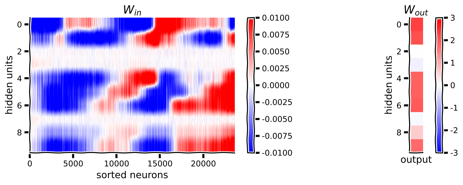
以下では、視覚野のニューロンから隠れユニットへの重み と、隠れユニットから出力の向きへの重み を可視化します。
PyTorchに関する注意:
以下のコードで重要なのは .detach() メソッドです。PyTorchの nn.Module クラスは特別で、その内部の変数は自動微分のために計算グラフで相互にリンクされています(.backward() で勾配を計算するアルゴリズムです)。そのため、nn.Module クラスのパラメータや出力に対して torch の操作以外の処理を行う場合は、まず計算グラフから「切り離す(detach)」必要があります。また、.cpu() メソッドでCPU上に「移す」必要があります。これが .detach() と .cpu() メソッドの役割です。以下のコードではネットワークの重みに対してこれを呼び出しています。さらに、PyTorchのテンソルをNumPy配列に変換するために .numpy() メソッドを使っています。
W_in = net.in_layer.weight.detach().cpu().numpy()  # we can run .detach(), .cpu() and .numpy() to get a numpy array
print(f'shape of W_in: {W_in.shape}')

W_out = net.out_layer.weight.detach().cpu().numpy()  # we can run .detach() .cpu() and .numpy() to get a numpy array
print(f'shape of W_out: {W_out.shape}')

plt.figure(figsize=(10, 4))
plt.subplot(121)
plt.imshow(W_in, aspect='auto', cmap='bwr', vmin=-1e-2, vmax=1e-2)
plt.xlabel('neurons')
plt.ylabel('hidden units')
plt.colorbar()
plt.title('$W_{in}$')

plt.subplot(122)
plt.imshow(W_out.T, cmap='bwr', vmin=-3, vmax=3)
plt.xticks([])
plt.xlabel('output')
plt.ylabel('hidden units')
plt.colorbar()
plt.title('$W_{out}$')

plt.show()
コーディング演習 1.1: 重みの可視化
この重み行列には構造が見えにくいです。より良い可視化方法はあるでしょうか?
おそらくニューロンをそれぞれの好みの向きでソートすると良いでしょう。360個の刺激(360度の角度)× ニューロン数の resp_all 行列を使います。好みの向きはどうやって見つけるでしょうか?
まずはこの resp_all 行列の1列を、ノートブックの最初で行ったように可視化してみましょう。好みの向きを決める前に、このチューニングカーブをどのように処理したいか見えてきますか?
idx = 235
plt.plot(resp_all[:, idx])
plt.ylabel('neural response')
plt.xlabel('stimulus orientation ($^\circ$)')
plt.title(f'neuron {idx}')
plt.show()
このチューニングカーブを見ると、向きごとに多少のノイズがあります。そこでガウシアンフィルターで平滑化し、各ニューロンの最大値の位置(すなわち「好みの向き」)を見つけます。最大値の位置はPythonの .argmax(axis=_) 関数で計算できます(軸を正しく指定してください)。次に、行列のインデックスをソートするには .argsort() 関数を使います。
from scipy.ndimage import gaussian_filter1d

# first let's smooth the tuning curves resp_all to make sure we get
# an accurate peak that isn't just noise
# resp_all is size (n_stimuli, n_neurons)
resp_smoothed = gaussian_filter1d(resp_all, 5, axis=0)
# resp_smoothed is size (n_stimuli, n_neurons)

############################################################################
## TO DO for students
# Fill out function and remove
raise NotImplementedError("Student exercise: find preferred orientation")
############################################################################

## find position of max response for each neuron
## aka preferred orientation for each neuron
preferred_orientation = ...

# Resort W_in matrix by preferred orientation
isort = preferred_orientation.argsort()
W_in_sorted = W_in[:, isort]

# plot resorted W_in matrix
visualize_weights(W_in_sorted, W_out)出力例:
# @title Submit your feedback
content_review(f"{feedback_prefix}_Visualizing_weights_Exercise")
さまざまな刺激に対する隠れユニットの活動をプロットすることで、隠れユニットの理解を深めることができます。隠れユニットの式を思い出してください。
と を使って活動 を直接計算することもできますし、上記のネットワークを修正して .forward() メソッドで h を返すようにすることもできます。ここでは式を使って計算しますが、実際には後者の方法が推奨されます。
W_in = net.in_layer.weight  # size (10, n_neurons)
b_in = net.in_layer.bias.unsqueeze(1)  # size (10, 1)

# Compute hidden unit activity h
h = torch.relu(W_in @ resp_all.T.to(device) + b_in)
h = h.detach().cpu().numpy()  # we can run .detach(), .cpu() and .numpy() to get a numpy array

# Visualize
visualize_hidden_units(W_in_sorted, h)
考えてみよう!1.1: 重みの解釈
モデルが神経活動を隠れ層の活動にどのように変換しているかを可視化しました。これらの行列をどのように解釈すべきでしょうか?以下のような問いを考えてみましょう。
- なぜ一部の隠れユニットに対して の重みがほぼゼロになっているのでしょうか?これらは の重みもほぼゼロに対応していますか?
- 各隠れユニットは、 の中で2つの異なる好みの向きを持つニューロン群に最も強い重みを持っているように見えます。これはなぜだと思いますか?ニューロンのチューニング曲線の構造について何を示唆しているでしょうか?
- 各向きに少なくとも1つの隠れユニットが活性化しているように見えますが、これはすべての向きをデコードするために必要です。もし一部の向きで隠れユニットが活性化しなかったらどうなるでしょうか?
# @title Submit your feedback
content_review(f"{feedback_prefix}_Interpreting_weights_Discussion")
セクション 1.2: テストデータによる一般化性能
勾配降下法は本質的にネットワークのパラメータを与えられた訓練データに適合させるアルゴリズムです。したがって、この訓練データの選択は、最適化されたパラメータが訓練されていない未知のデータに対しても一般化できることを保証するために非常に重要です。例えば今回の場合、訓練されたネットワークがデータセット内の向きだけでなく、任意の刺激の向きから神経応答を正しくデコードできることを確認したいわけです。
これを保証するために、全データセットを訓練セットとテストセットに分割しています。コーディング演習3.2では、訓練セットでパラメータを最適化して深層ネットワークを訓練しました。ここでは、訓練済みネットワークを使ってテストセットの神経応答から刺激の向きをデコードし、最適化されたパラメータの性能を評価します。このテストセットでの良好なデコード性能は、他の任意の刺激向きに対する神経応答でも良好な性能を示すことの指標となります。この手法は機械学習(深層学習に限らず)で一般的に用いられ、交差検証と呼ばれます。
テストデータに対する平均二乗誤差(MSE)を計算し、真の刺激向きに対するデコードされた刺激向きをプロットします。
# @markdown Execute this cell to evaluate and plot test error

out = net(resp_test.to(device))  # decode stimulus orientation for neural responses in testing set
ori = stimuli_test  # true stimulus orientations
test_loss = loss_fn(out.to(device), ori.to(device))  # MSE on testing set (Hint: use loss_fn initialized in previous exercise)

plt.plot(ori, out.detach().cpu(), '.')  # N.B. need to use .detach() to pass network output into plt.plot()
identityLine()  # draw the identity line y=x; deviations from this indicate bad decoding!
plt.title(f'MSE on testing set: {test_loss.item():.2f}')  # N.B. need to use .item() to turn test_loss into a scalar
plt.xlabel('true stimulus orientation ($^o$)')
plt.ylabel('decoded stimulus orientation ($^o$)')
axticks = np.linspace(0, 360, 5)
plt.xticks(axticks)
plt.yticks(axticks)
plt.show()
興味があれば、次のセクションでモデル批判についてさらに考え、損失関数を改善し、正則化を追加する方法について学んでください。
セクション 2: デコーディング - モデルの評価と改善
セクション 2.1: モデル批判
ここで一歩引いて、私たちのモデルがどのように成功または失敗しているのか、そしてどのように改善できるかを考えてみましょう。
# @markdown Execute this cell to plot decoding error

out = net(resp_test.to(device)).to(device)  # decode stimulus orientation for neural responses in testing set
ori = stimuli_test.to(device)  # true stimulus orientations
error = out - ori  # decoding error


plt.plot(ori.detach().cpu(), error.detach().cpu(), '.')   # plot decoding error as a function of true orientation (make sure all arguments to plt.plot() have been detached from PyTorch network!)

# Plotting
plt.xlabel('true stimulus orientation ($^o$)')
plt.ylabel('decoding error ($^o$)')
plt.xticks(np.linspace(0, 360, 5))
plt.yticks(np.linspace(-360, 360, 9))
plt.show()
考えてみよう!2.1: エラー問題の掘り下げ
以下のセルでは、テストセットの各ニューロン応答に対するデコーディング誤差をプロットします。デコーディング誤差は、デコードされた刺激の向きから真の刺激の向きを引いたものとして定義されます。
特に、真の刺激の向きを横軸にしてデコーディング誤差をプロットします。
- ある刺激の向きは他の向きよりもデコードが難しいですか?
- もしそうなら、どのような意味で?これらの刺激のデコードされた向きはよりばらつきが大きいですか、それとも偏りがありますか?
- このばらつきや偏りを説明できますか?これらの刺激の向きは他と何が違うのでしょうか?
- (次の演習で扱います)この問題を避けるためにディープネットワークをどのように修正できるか考えられますか?
# @title Submit your feedback
content_review(f"{feedback_prefix}_Delving_into_error_problems_Discussion")
セクション 2.2: 損失関数の改善
前の演習で示したように、二乗誤差は角度のような円環状の量には適した損失関数ではありません。というのも、非常に近い角度(例えば と )でも、二乗誤差は非常に大きくなってしまう可能性があるからです。
ここでは、この問題を回避するために、損失関数を変更してデコーディング問題を分類問題として扱います。刺激の正確な角度を推定するのではなく、角度を幅 の異なるビンに分けた クラスのいずれかに刺激を分類するデコーダを構築することを目指します。刺激 の真のクラス は次のように定義されます。
刺激の向きから 個の刺激クラスを抽出するヘルパー関数 stimulus_class を用意しています。
神経応答から刺激クラスをデコードするために、次元の確率ベクトル を出力するディープネットワークを使います。ここで、 は刺激がクラス のいずれかに属する確率の推定値です。
ネットワークの出力が確かに確率(すなわち、0から1の間の正の数であり、合計が1になる)となるように、ソフトマックス関数$を用いて隠れ層からの実数値の出力を確率に変換します。ソフトマックス関数を と表すと、ネットワークの数式は以下のようになります。
\begin{align}
&= && [: M ], \
&= && [: C ],
\end{align}
デコードされた刺激クラスは、ネットワークが最も高い確率を割り当てたクラスとなります:
PyTorchでは、torch.softmax() を使ってソフトマックス関数を簡単に実装できます。
実際の確率よりも 対数 確率の方が扱いやすいことが多いです。なぜなら確率は非常に小さい数値になりがちで、コンピュータが表現しづらいためです。そこで、ネットワークの出力としてソフトマックスの対数を用います。
これは PyTorch の nn.LogSoftmax レイヤーを使ってソフトマックスと一緒に実装できます。対数関数の良い点は単調性があることです。つまり、ある確率が別の確率より大きい/小さい場合、その対数も同様に大きい/小さいということです。したがって、
次のセルでは、ReLUを1層持つ隠れ層を持つディープネットワークを構築し、対数確率のベクトルを出力するコードを示します。
# Deep network for classification
class DeepNetSoftmax(nn.Module):
  """Deep Network with one hidden layer, for classification

  Args:
    n_inputs (int): number of input units
    n_hidden (int): number of units in hidden layer
    n_classes (int): number of outputs, i.e. number of classes to output
      probabilities for

  Attributes:
    in_layer (nn.Linear): weights and biases of input layer
    out_layer (nn.Linear): weights and biases of output layer

  """

  def __init__(self, n_inputs, n_hidden, n_classes):
    super().__init__()  # needed to invoke the properties of the parent class nn.Module
    self.in_layer = nn.Linear(n_inputs, n_hidden)  # neural activity --> hidden units
    self.out_layer = nn.Linear(n_hidden, n_classes)  # hidden units --> outputs
    self.logprob = nn.LogSoftmax(dim=1)  # probabilities across columns should sum to 1 (each output row corresponds to a different input)

  def forward(self, r):
    """Predict stimulus orientation bin from neural responses

    Args:
      r (torch.Tensor): n_stimuli x n_inputs tensor with neural responses to n_stimuli

    Returns:
      torch.Tensor: n_stimuli x n_classes tensor with predicted class probabilities

    """
    h = torch.relu(self.in_layer(r))
    logp = self.logprob(self.out_layer(h))
    return logp
損失関数は何にすべきでしょうか?理想的には、ネットワークの出力する確率が真の刺激クラスの確率を高くすることです。これを形式化すると、ネットワークが予測したクラス確率の下で、真の刺激クラス の 対数 確率を最大化したいということになります。
これを最小化すべき損失関数に変換するために、単に -1 をかけます。対数確率を最大化することは、負の対数確率を最小化することと同じです。バッチサイズ の入力に対して合計すると、損失関数は次のようになります。
ディープラーニングの分野では、この損失関数は通常 クロスエントロピー または 負の対数尤度 と呼ばれます。PyTorchの対応する組み込み損失関数は nn.NLLLoss() です(ドキュメントはこちら)。
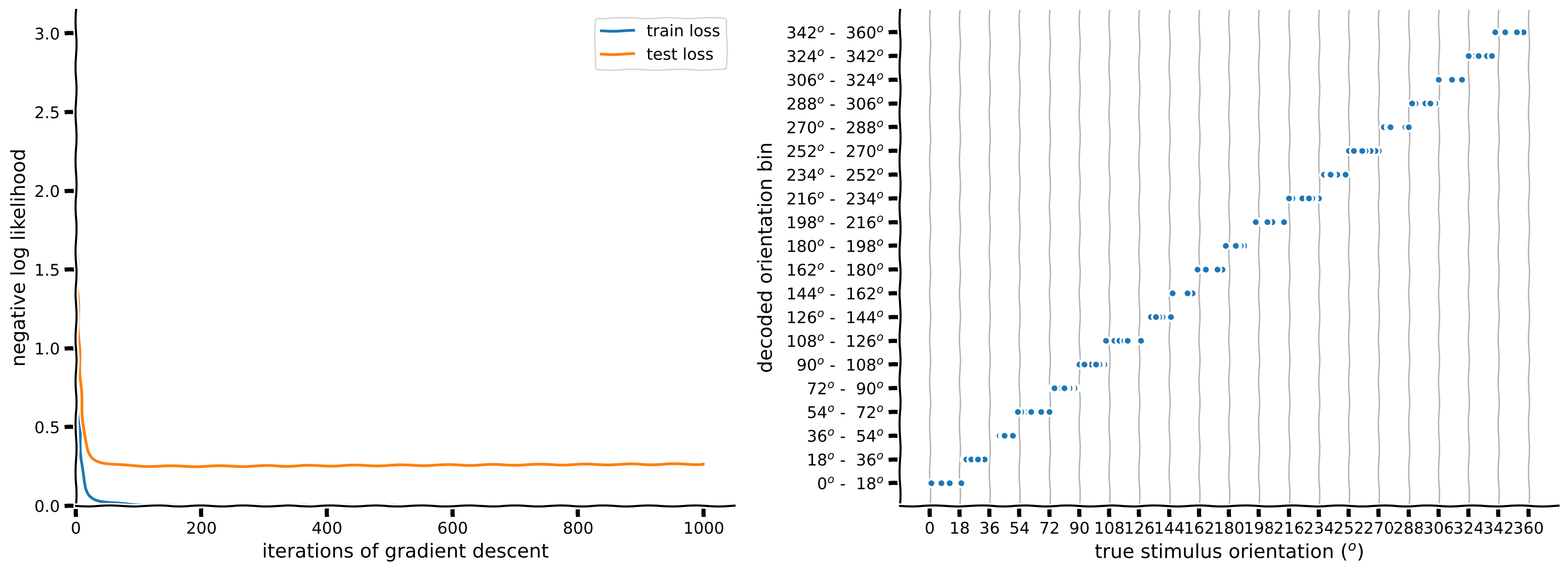
コーディング演習 2.2: 新しい損失関数
次のセルでは、負の対数尤度を最小化することで刺激の向きを分類によってデコードするネットワークの学習とテストのコードのほとんどを用意しています。欠けている部分を埋めてください。
これができたら、プロットされた結果を見てみましょう。損失関数を平均二乗誤差から分類損失に変えることで、問題は解決しましたか?誤りはまだ起こるかもしれませんが、それらの誤りは上記のネットワークが犯していた誤りと比べてどの程度悪いでしょうか?
# @markdown Run this cell to create train function that uses test_data and L1 and L2 terms for next exercise
def train(net, loss_fn, train_data, train_labels,
          n_iter=50, learning_rate=1e-4,
          test_data=None, test_labels=None,
          L2_penalty=0, L1_penalty=0):
  """Run gradient descent to optimize parameters of a given network

  Args:
    net (nn.Module): PyTorch network whose parameters to optimize
    loss_fn: built-in PyTorch loss function to minimize
    train_data (torch.Tensor): n_train x n_neurons tensor with neural
      responses to train on
    train_labels (torch.Tensor): n_train x 1 tensor with orientations of the
      stimuli corresponding to each row of train_data
    n_iter (int, optional): number of iterations of gradient descent to run
    learning_rate (float, optional): learning rate to use for gradient descent
    test_data (torch.Tensor, optional): n_test x n_neurons tensor with neural
      responses to test on
    test_labels (torch.Tensor, optional): n_test x 1 tensor with orientations of
      the stimuli corresponding to each row of test_data
    L2_penalty (float, optional): l2 penalty regularizer coefficient
    L1_penalty (float, optional): l1 penalty regularizer coefficient

  Returns:
    (list): training loss over iterations

  """

  # Initialize PyTorch SGD optimizer
  optimizer = optim.SGD(net.parameters(), lr=learning_rate)

  # Placeholder to save the loss at each iteration
  train_loss = []
  test_loss = []

  # Loop over epochs
  for i in range(n_iter):

    # compute network output from inputs in train_data
    out = net(train_data)  # compute network output from inputs in train_data

    # evaluate loss function
    if L2_penalty==0 and L1_penalty==0:
      # normal loss function
      loss = loss_fn(out, train_labels)
    else:
      # custom loss function from bonus exercise 3.3
      loss = loss_fn(out, train_labels, net.in_layer.weight,
                     L2_penalty, L1_penalty)

    # Clear previous gradients
    optimizer.zero_grad()
    # Compute gradients
    loss.backward()

    # Update weights
    optimizer.step()

    # Store current value of loss
    train_loss.append(loss.item())  # .item() needed to transform the tensor output of loss_fn to a scalar

    # Get loss for test_data, if given (we will use this in the bonus exercise 3.2 and 3.3)
    if test_data is not None:
      out_test = net(test_data)
      # evaluate loss function
      if L2_penalty==0 and L1_penalty==0:
        # normal loss function
        loss_test = loss_fn(out_test, test_labels)
      else:
        # (BONUS code) custom loss function from Bonus exercise 3.3
        loss_test = loss_fn(out_test, test_labels, net.in_layer.weight,
                            L2_penalty, L1_penalty)
      test_loss.append(loss_test.item())  # .item() needed to transform the tensor output of loss_fn to a scalar

    # Track progress
    if (i + 1) % (n_iter // 5) == 0:
      if test_data is None:
        print(f'iteration {i + 1}/{n_iter} | loss: {loss.item():.3f}')
      else:
        print(f'iteration {i + 1}/{n_iter} | loss: {loss.item():.3f} | test_loss: {loss_test.item():.3f}')

  if test_data is None:
    return train_loss
  else:
    return train_loss, test_loss
def decode_orientation(net, n_classes, loss_fn,
train_data, train_labels, test_data, test_labels,
n_iter=1000, L2_penalty=0, L1_penalty=0, device='cpu'):
""" Initialize, train, and test deep network to decode binned orientation from neural responses
Args:
net (nn.Module): deep network to run
n_classes (scalar): number of classes in which to bin orientation
loss_fn (function): loss function to run
train_data (torch.Tensor): n_train x n_neurons tensor with neural
responses to train on
train_labels (torch.Tensor): n_train x 1 tensor with orientations of the
stimuli corresponding to each row of train_data, in radians
test_data (torch.Tensor): n_test x n_neurons tensor with neural
responses to train on
test_labels (torch.Tensor): n_test x 1 tensor with orientations of the
stimuli corresponding to each row of train_data, in radians
n_iter (int, optional): number of iterations to run optimization
L2_penalty (float, optional): l2 penalty regularizer coefficient
L1_penalty (float, optional): l1 penalty regularizer coefficient
Returns:
(list, torch.Tensor): training loss over iterations, n_test x 1 tensor with predicted orientations of the
stimuli from decoding neural network
"""
# Bin stimulus orientations in training set
train_binned_labels = stimulus_class(train_labels, n_classes).to(device)
test_binned_labels = stimulus_class(test_labels, n_classes).to(device)
train_data = train_data.to(device)
test_data = test_data.to(device)
# Run GD on training set data, using learning rate of 0.1
# (add optional arguments test_data and test_binned_labels!)
train_loss, test_loss = train(net.to(device), loss_fn, train_data, train_binned_labels,
learning_rate=0.1, test_data=test_data,
test_labels=test_binned_labels, n_iter=n_iter,
L2_penalty=L2_penalty, L1_penalty=L1_penalty)
# Decode neural responses in testing set data
out = net(test_data).to(device)
out_labels = np.argmax(out.detach().cpu(), axis=1) # predicted classes
frac_correct = (out_labels == test_binned_labels.cpu()).sum() / len(test_binned_labels)
print(f'>>> fraction correct = {frac_correct:.3f}')
return train_loss, test_loss, out_labels
# Set random seeds for reproducibility
np.random.seed(1)
torch.manual_seed(1)
n_classes = 20
############################################################################
## TO DO for students
# Fill out function and remove
raise NotImplementedError("Student exercise: make network and loss")
############################################################################
# Initialize network
net = ... # use M=20 hidden units
# Initialize built-in PyTorch negative log likelihood loss function
loss_fn = ...
# Train network and run it on test images
# this function uses the train function you wrote before
train_loss, test_loss, predicted_test_labels = decode_orientation(net, n_classes, loss_fn.to(device),
resp_train, stimuli_train,
resp_test, stimuli_test,
device=device)
# Plot results
plot_decoded_results(train_loss, test_loss, stimuli_test, predicted_test_labels, n_classes)出力例:
# @title Submit your feedback
content_review(f"{feedback_prefix}_A_new_loss_function_Exercise")
ニューロンから隠れ層への重み は今どのようになっていますか?
W_in = net.in_layer.weight.detach().cpu().numpy() # we can run detach, cpu and numpy to get a numpy array
print(f'shape of W_in: {W_in.shape}')

W_out = net.out_layer.weight.detach().cpu().numpy()

# plot resorted W_in matrix
visualize_weights(W_in[:, isort], W_out)
セクション 2.3: 正則化
# @title Video 1: Regularization
from ipywidgets import widgets
from IPython.display import YouTubeVideo
from IPython.display import IFrame
from IPython.display import display


class PlayVideo(IFrame):
  def __init__(self, id, source, page=1, width=400, height=300, **kwargs):
    self.id = id
    if source == 'Bilibili':
      src = f'https://player.bilibili.com/player.html?bvid={id}&page={page}'
    elif source == 'Osf':
      src = f'https://mfr.ca-1.osf.io/render?url=https://osf.io/download/{id}/?direct%26mode=render'
    super(PlayVideo, self).__init__(src, width, height, **kwargs)


def display_videos(video_ids, W=400, H=300, fs=1):
  tab_contents = []
  for i, video_id in enumerate(video_ids):
    out = widgets.Output()
    with out:
      if video_ids[i][0] == 'Youtube':
        video = YouTubeVideo(id=video_ids[i][1], width=W,
                             height=H, fs=fs, rel=0)
        print(f'Video available at https://youtube.com/watch?v={video.id}')
      else:
        video = PlayVideo(id=video_ids[i][1], source=video_ids[i][0], width=W,
                          height=H, fs=fs, autoplay=False)
        if video_ids[i][0] == 'Bilibili':
          print(f'Video available at https://www.bilibili.com/video/{video.id}')
        elif video_ids[i][0] == 'Osf':
          print(f'Video available at https://osf.io/{video.id}')
      display(video)
    tab_contents.append(out)
  return tab_contents


video_ids = [('Youtube', 'Qnn5OPHKo5w'), ('Bilibili', 'BV1na4y1a7ug')]
tab_contents = display_videos(video_ids, W=854, H=480)
tabs = widgets.Tab()
tabs.children = tab_contents
for i in range(len(tab_contents)):
  tabs.set_title(i, video_ids[i][0])
display(tabs)
# @title Submit your feedback
content_review(f"{feedback_prefix}_Regularization_Video")講義で説明したように、過学習を避けるために損失関数に正則化項を組み込むことが重要な場合がよくあります。特に今回は、ニューロンから隠れユニットへの線形層にスパース性を強制するためにこれらの項を使用します。
ここでは、古典的なL2正則化ペナルティ を考えます。これはネットワーク内の各重みの二乗和 に定数 L2_penalty を掛けたものです。
また、重みのスパース性を強制するためにL1正則化ペナルティ も加えます。これは重みの絶対値の和 に定数 L1_penalty を掛けたものです。
これら両方を損失関数に加えます:
パラメータ L2_penalty と L1_penalty は train 関数への入力です。
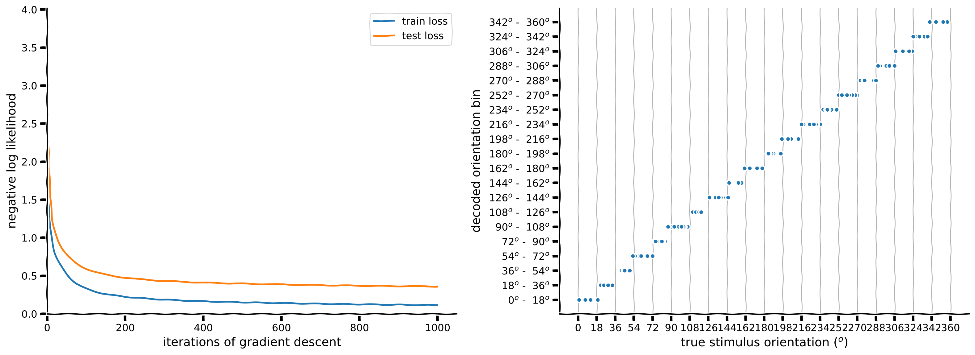
コーディング演習 2.3: トレーニングに正則化を追加する
L1およびL2正則化を加えた新しい損失関数を作成します。
具体的には、
- 重みにL2損失ペナルティを追加する
- 重みにL1損失ペナルティを追加する
この損失関数を使ってネットワークをトレーニングします。完全なトレーニングには数分かかります。コードの反復を速めるために数ステップだけトレーニングしたい場合は、n_iter の入力値を500から減らすことができます。
ヒント:npではなくtorchを使っているので、np.absoluteの代わりにtorch.absを使います。テンソルの合計にはtorch.sumまたは.sum()を使えます。
def regularized_loss(output, target, weights, L2_penalty=0, L1_penalty=0,
                     device='cpu'):
  """loss function with L2 and L1 regularization

  Args:
    output (torch.Tensor): output of network
    target (torch.Tensor): neural response network is trying to predict
    weights (torch.Tensor): linear layer weights from neurons to hidden units (net.in_layer.weight)
    L2_penalty : scaling factor of sum of squared weights
    L1_penalty : scaling factor for sum of absolute weights

  Returns:
    (torch.Tensor) mean-squared error with L1 and L2 penalties added

  """

  ##############################################################################
  # TO DO: add L1 and L2 regularization to the loss function
  raise NotImplementedError("Student exercise: complete regularized_loss")
  ##############################################################################

  loss_fn = nn.NLLLoss()
  loss = loss_fn(output, target)

  L2 = L2_penalty * ...
  L1 = L1_penalty * ...
  loss += L1 + L2

  return loss.to(device)


# Set random seeds for reproducibility
np.random.seed(1)
torch.manual_seed(1)

n_classes = 20

# Initialize network
net = DeepNetSoftmax(n_neurons, 20, n_classes)  # use M=20 hidden units

# Here you can play with L2_penalty > 0, L1_penalty > 0
train_loss, test_loss, predicted_test_labels = decode_orientation(net, n_classes,
                                                                  regularized_loss,
                                                                  resp_train, stimuli_train,
                                                                  resp_test, stimuli_test,
                                                                  n_iter=1000,
                                                                  L2_penalty=1e-2,
                                                                  L1_penalty=5e-4,
                                                                  device=device)

# Plot results
plot_decoded_results(train_loss, test_loss, stimuli_test, predicted_test_labels, n_classes)出力例:
# @title Submit your feedback
content_review(f"{feedback_prefix}_Add_regularization_to_training_Exercise")
L1およびL2正則化ペナルティを加えたことで精度が少し向上したため、少し過学習していたようです。モデルはまだどのような誤りを犯しているでしょうか?
L1_penalty > 0 を加えた後の重みの様子を見てみましょう。
W_in = net.in_layer.weight.detach().cpu().numpy()  # we can run detach, cpu and numpy to get a numpy array
print(f'shape of W_in: {W_in.shape}')

W_out = net.out_layer.weight.detach().cpu().numpy()

visualize_weights(W_in[:, isort], W_out)
重みは以前よりもスパースになっているようです。
セクション3: エンコーディング - エンコーディングのための畳み込みネットワーク
# @title Video 2: Convolutional Encoding Model
from ipywidgets import widgets
from IPython.display import YouTubeVideo
from IPython.display import IFrame
from IPython.display import display


class PlayVideo(IFrame):
  def __init__(self, id, source, page=1, width=400, height=300, **kwargs):
    self.id = id
    if source == 'Bilibili':
      src = f'https://player.bilibili.com/player.html?bvid={id}&page={page}'
    elif source == 'Osf':
      src = f'https://mfr.ca-1.osf.io/render?url=https://osf.io/download/{id}/?direct%26mode=render'
    super(PlayVideo, self).__init__(src, width, height, **kwargs)


def display_videos(video_ids, W=400, H=300, fs=1):
  tab_contents = []
  for i, video_id in enumerate(video_ids):
    out = widgets.Output()
    with out:
      if video_ids[i][0] == 'Youtube':
        video = YouTubeVideo(id=video_ids[i][1], width=W,
                             height=H, fs=fs, rel=0)
        print(f'Video available at https://youtube.com/watch?v={video.id}')
      else:
        video = PlayVideo(id=video_ids[i][1], source=video_ids[i][0], width=W,
                          height=H, fs=fs, autoplay=False)
        if video_ids[i][0] == 'Bilibili':
          print(f'Video available at https://www.bilibili.com/video/{video.id}')
        elif video_ids[i][0] == 'Osf':
          print(f'Video available at https://osf.io/{video.id}')
      display(video)
    tab_contents.append(out)
  return tab_contents


video_ids = [('Youtube', 'UNBOPZf0QNQ'), ('Bilibili', 'BV1Eh41167WP')]
tab_contents = display_videos(video_ids, W=854, H=480)
tabs = widgets.Tab()
tabs.children = tab_contents
for i in range(len(tab_contents)):
  tabs.set_title(i, video_ids[i][0])
display(tabs)
# @title Submit your feedback
content_review(f"{feedback_prefix}_Convolutional_Encoding_Model_Video")神経科学では、脳が外部刺激をどのように表現しているかを理解したいことがよくあります。これらの表現を発見する一つの方法は、外部刺激(この場合は格子刺激)を入力として受け取り、神経応答を出力するエンコーディングモデルを構築することです。
視覚野はしばしば視野全体で同じフィルターが組み合わされる畳み込みネットワークと考えられているため、畳み込み層を持つモデルを使用します。前のセクションで畳み込み層の構築方法を学びました。この畳み込み層に加えて、畳み込みの出力からニューロンへの全結合層を追加します。その後、この全結合層の重みを可視化します。
# @markdown Execute this cell to download the data
import hashlib
import requests

fname = "W3D4_stringer_oribinned6_split.npz"
url = "https://osf.io/p3aeb/download"
expected_md5 = "b3f7245c6221234a676b71a1f43c3bb5"

if not os.path.isfile(fname):
  try:
    r = requests.get(url)
  except requests.ConnectionError:
    print("!!! Failed to download data !!!")
  else:
    if r.status_code != requests.codes.ok:
      print("!!! Failed to download data !!!")
    elif hashlib.md5(r.content).hexdigest() != expected_md5:
      print("!!! Data download appears corrupted !!!")
    else:
      with open(fname, "wb") as fid:
        fid.write(r.content)
セクション3.1: ニューロンのチューニング曲線
次のセルでは、ランダムに選んだニューロンのチューニング曲線をプロットします。チュートリアル1よりも刺激の向きを細かくビニングしています。以下の60の向きに対して上記と同様に格子画像を作成し、変数grating_stimuliに保存します。
セルを再実行して異なる例のニューロンを見て、集団内のチューニング曲線の多様性を観察してください。これらの神経応答をエンコーディングモデルでどのようにフィットできるでしょうか?
# @markdown Execute this cell to load data, create stimuli, and plot neural tuning curves

### Load data and bin at 8 degrees
# responses are split into test and train
resp_train, resp_test, stimuli = load_data_split(fname)
n_stimuli, n_neurons = resp_train.shape
print(f'resp_train contains averaged responses of {n_neurons} neurons'
      f'to {n_stimuli} binned stimuli')

# also make stimuli into images
orientations = np.linspace(0, 360, 61)[:-1] - 180
grating_stimuli = np.zeros((60, 1, 12, 16), np.float32)
for i, ori in enumerate(orientations):
  grating_stimuli[i,0] = grating(ori, res=0.025)#[18:30, 24:40]

grating_stimuli = torch.from_numpy(grating_stimuli)
print('grating_stimuli contains 60 stimuli of size 12 x 16')

# Visualize tuning curves
fig, axs = plt.subplots(3, 5, figsize=(15,7))
for k, ax in enumerate(axs.flatten()):
  neuron_index = np.random.choice(n_neurons)  # pick random neuron
  plot_tuning(ax, stimuli, resp_train[:, neuron_index], resp_test[:, neuron_index], neuron_index, linewidth=2)
  if k == 0:
    ax.text(1.0, 0.9, 'train', color='y', transform=ax.transAxes)
    ax.text(1.0, 0.65, 'test', color='m', transform=ax.transAxes)

fig.tight_layout()
plt.show()
セクション3.2: エンコーディングモデルを作るために全結合層を追加する
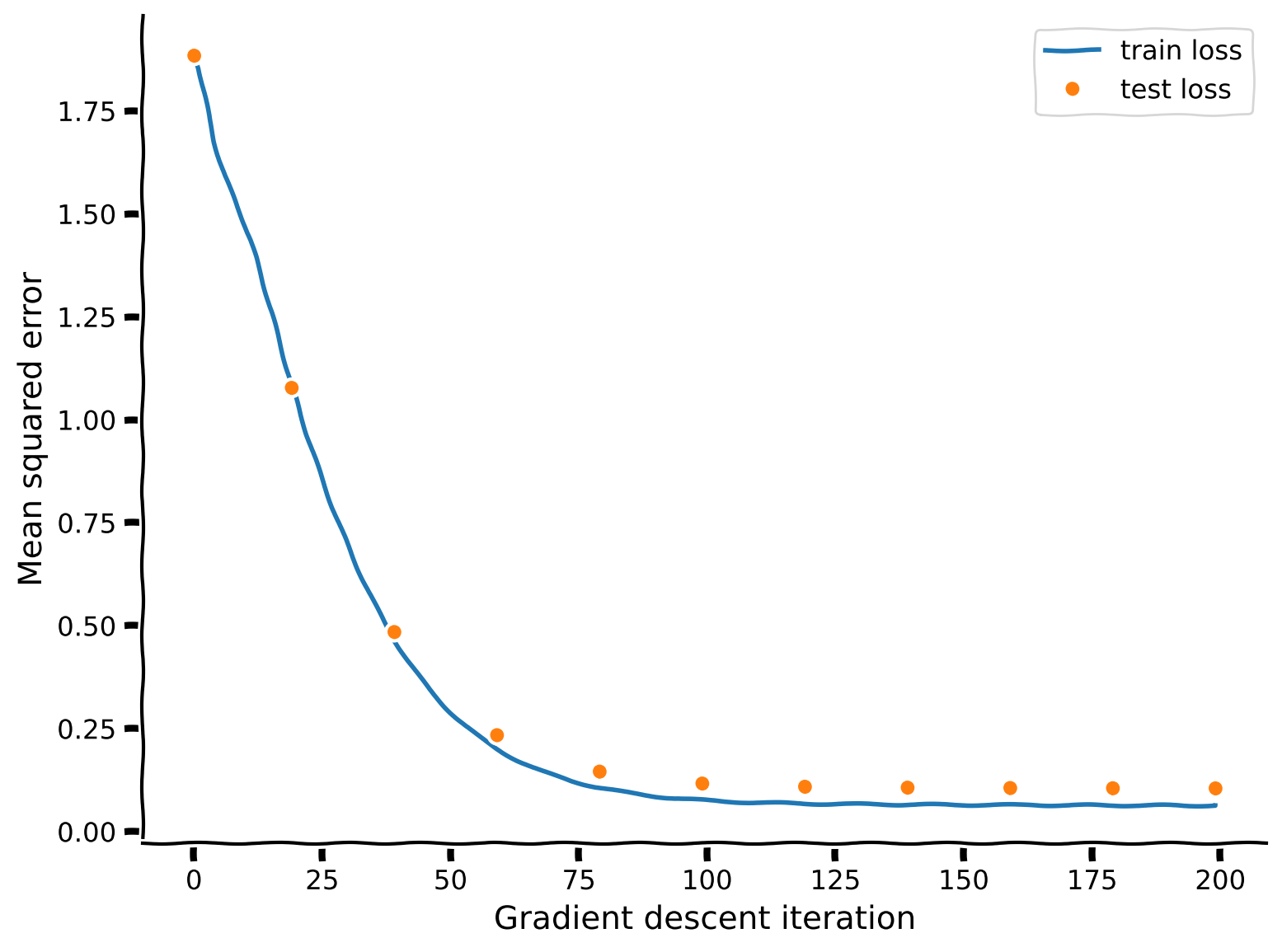
上記と同様に畳み込み層を持つtorchモデルを構築します。さらに、畳み込みユニットからニューロンへの全結合線形層を追加します。畳み込みチャネル数()は6、カーネルサイズ()は7、ストライドは1、パディングは(上記と同じ)を使用します。刺激のサイズは(12, 16)です。畳み込みユニットの活性化は線形層を通って神経応答に変換されます。
考えてみよう!3.2: ユニット数と重みの数
- 畳み込み層のユニット数はいくつになるでしょうか?
- 畳み込みユニットからニューロンへの全結合線形層の重みはいくつになるでしょうか?
# @title Submit your feedback
content_review(f"{feedback_prefix}_Number_of_units_and_weights_Discussion")
コーディング演習 3.2: 線形層を追加しよう
チュートリアル1で線形層を使ったことを思い出してください。チュートリアル1の知識を活かして、上で作成したモデルに線形層を追加しましょう。
# @markdown Execute to get `train` function for our neural encoding model

def train(net, custom_loss, train_data, train_labels,
          test_data=None, test_labels=None,
          learning_rate=10, n_iter=500, L2_penalty=0., L1_penalty=0.):
  """Run gradient descent for network without batches

  Args:
    net (nn.Module): deep network whose parameters to optimize with SGD
    custom_loss: loss function for network
    train_data: training data (n_train x input features)
    train_labels: training labels (n_train x output features)
    test_data: test data (n_train x input features)
    test_labels: test labels (n_train x output features)
    learning_rate (float): learning rate for gradient descent
    n_epochs (int): number of epochs to run gradient descent
    L2_penalty (float): magnitude of L2 penalty
    L1_penalty (float): magnitude of L1 penalty

  Returns:
    train_loss: training loss across iterations
    test_loss: testing loss across iterations

  """
  optimizer = optim.SGD(net.parameters(), lr=learning_rate, momentum=0.9) # Initialize PyTorch SGD optimizer
  train_loss = np.nan * np.zeros(n_iter)  # Placeholder for train loss
  test_loss = np.nan * np.zeros(n_iter)  # Placeholder for test loss

  # Loop over epochs
  for i in range(n_iter):
    if n_iter < 10:
      for param_group in self.optimizer.param_groups:
        param_group['lr'] = np.linspace(0, learning_rate, 10)[n_iter]
    y_pred = net(train_data) # Forward pass: compute predicted y by passing train_data to the model.

    if L2_penalty>0 or L1_penalty>0:
      weights = net.out_layer.weight
      loss = custom_loss(y_pred, train_labels, weights, L2_penalty, L1_penalty)
    else:
      loss = custom_loss(y_pred, train_labels)

    ### Update parameters
    optimizer.zero_grad() # zero out gradients
    loss.backward() # Backward pass: compute gradient of the loss with respect to model parameters
    optimizer.step() # step parameters in gradient direction
    train_loss[i] = loss.item()  # .item() transforms the tensor to a scalar and does .detach() for us

    # Track progress
    if (i+1) % (n_iter // 10) == 0 or i==0:
      if test_data is not None and test_labels is not None:
        y_pred = net(test_data)
        if L2_penalty>0 or L1_penalty>0:
          loss = custom_loss(y_pred, test_labels, weights, L2_penalty, L1_penalty)
        else:
          loss = custom_loss(y_pred, test_labels)
        test_loss[i] = loss.item()
        print(f'iteration {i+1}/{n_iter} | train loss: {train_loss[i]:.4f} | test loss: {test_loss[i]:.4f}')
      else:
        print(f'iteration {i+1}/{n_iter} | train loss: {train_loss[i]:.4f}')

  return train_loss, test_loss
class ConvFC(nn.Module):
"""Deep network with one convolutional layer + one fully connected layer
Attributes:
conv (nn.Conv1d): convolutional layer
dims (tuple): shape of convolutional layer output
out_layer (nn.Linear): linear layer
"""
def __init__(self, n_neurons, c_in=1, c_out=6, K=7, b=12*16,
filters=None):
""" initialize layer
Args:
c_in: number of input stimulus channels
c_out: number of convolutional channels
K: size of each convolutional filter
h: number of stimulus bins, n_bins
"""
super().__init__()
self.conv = nn.Conv2d(c_in, c_out, kernel_size=K, padding=K//2, stride=1)
self.dims = (c_out, b) # dimensions of conv layer output
M = np.prod(self.dims) # number of hidden units
################################################################################
## TO DO for students: add fully connected layer to network (self.out_layer)
# Fill out function and remove
raise NotImplementedError("Student exercise: add fully connected layer to initialize network")
################################################################################
self.out_layer = nn.Linear(M, ...)
# initialize weights
if filters is not None:
self.conv.weight = nn.Parameter(filters)
self.conv.bias = nn.Parameter(torch.zeros((c_out,), dtype=torch.float32))
nn.init.normal_(self.out_layer.weight, std=0.01) # initialize weights to be small
def forward(self, s):
""" Predict neural responses to stimuli s
Args:
s (torch.Tensor): n_stimuli x c_in x h x w tensor with stimuli
Returns:
y (torch.Tensor): n_stimuli x n_neurons tensor with predicted neural responses
"""
a = self.conv(s) # output of convolutional layer
a = a.view(-1, np.prod(self.dims)) # flatten each convolutional layer output into a vector
################################################################################
## TO DO for students: add fully connected layer to forward pass of network (self.out_layer)
# Fill out function and remove
raise NotImplementedError("Student exercise: add fully connected layer to network")
################################################################################
y = ...
return y
# Initialize network
n_neurons = resp_train.shape[1]
## Initialize with filters from Tutorial 2
example_filters = filters(out_channels=6, K=7)
net = ConvFC(n_neurons, filters = example_filters).to(device)
# Run GD on training set data
# ** this time we are also providing the test data to estimate the test loss
train_loss, test_loss = train(net, regularized_MSE_loss,
train_data=grating_stimuli.to(device), train_labels=resp_train.to(device),
test_data=grating_stimuli.to(device), test_labels=resp_test.to(device),
n_iter=200, learning_rate=2,
L2_penalty=5e-4, L1_penalty=1e-6)
# Visualize
plot_training_curves(train_loss, test_loss)出力例:
# @title Submit your feedback
content_review(f"{feedback_prefix}_Add_linear_layer_Exercise")
このモデルで単一ニューロンのチューニング曲線をどの程度フィットできるでしょうか?チューニング曲線のどの側面を捉えているでしょうか?
# @markdown Execute this cell to examine predictions for random subsets of neurons

y_pred = net(grating_stimuli.to(device))
# Visualize tuning curves & plot neural predictions
fig, axs = plt.subplots(2, 5, figsize=(15,6))
for k, ax in enumerate(axs.flatten()):
  ineur = np.random.choice(n_neurons)
  plot_prediction(ax, y_pred[:, ineur].detach().cpu(),
                  resp_train[:, ineur],
                  resp_test[:, ineur])
  if k==0:
    ax.text(.1, 1., 'train', color='y', transform=ax.transAxes)
    ax.text(.1, 0.9, 'test', color='m', transform=ax.transAxes)
    ax.text(.1, 0.8, 'prediction', color='g', transform=ax.transAxes)

fig.tight_layout()
plt.show()
畳み込みチャネルが初期化時の中心周辺型やガボールフィルターから変化したかどうかを確認できます。もし変化していなければ、それはこれらのフィルターが上記で見られた精度でニューロンの向きに対する応答を説明するのに十分な基底セットであったことを意味します。
# get weights of conv layer in convLayer
out_channels = 6  # how many convolutional channels to have in our layer
weights = net.conv.weight.detach().cpu()
print(weights.shape)  # Can you identify what each of the dimensions are?

plot_weights(weights, channels=np.arange(0, out_channels))