チュートリアル 3: 規範的符号化モデルの構築と評価

第1週, 5日目: 深層学習

Neuromatch Academyによる

コンテンツ作成者: Jorge A. Menendez, Yalda Mohsenzadeh, Carsen Stringer

コンテンツレビュアー: Roozbeh Farhoodi, Madineh Sarvestani, Kshitij Dwivedi, Spiros Chavlis, Ella Batty, Michael Waskom

制作編集者: Spiros Chavlis

チュートリアルの目的

推定所要時間: 1時間10分

このチュートリアルでは、深層学習を用いて視覚系の符号化モデルを構築し、その内部表現を神経データで観察された表現と比較します。

モデルのパラメータは神経データに直接フィットするようには最適化しません。代わりに、脳が解くことができる特定の視覚課題を解くようにパラメータを最適化します。したがって、これは特定の行動課題に最適化されたため、**「規範的」**符号化モデルと呼びます。これは問題を解くための最適モデルです（指定されたアーキテクチャに対して最適）。畳み込みニューラルネットワークを神経データに直接フィットさせる方法（深層ニューラルネットワークによる符号化の別アプローチ）については、ボーナスチュートリアルのセクション3を参照してください。

この規範的符号化モデルが実際に脳の良いモデルであるか評価するために、その内部表現を解析し、マウスの一次視覚野で観察された表現と比較します。符号化モデルの表現が何に最適化されているかを正確に理解しているため、類似点は脳内の表現がなぜそのような形をしているのかを解明する手がかりになることが期待されます。

具体的には、以下を学ぶことを目標とします。

深層ネットワークの内部表現を可視化・解析する方法
表現類似性解析（Representational Similarity Analysis, RSA）を用いて、モデルの分散表現と神経記録で観察された神経表現の類似度を定量化する方法

# @title Tutorial slides
# @markdown These are the slides for all videos in this tutorial.
from IPython.display import IFrame
link_id = "kwyvp"
print(f"If you want to download the slides: https://osf.io/download/{link_id}/")
IFrame(src=f"https://mfr.ca-1.osf.io/render?url=https://osf.io/{link_id}/?direct%26mode=render%26action=download%26mode=render", width=854, height=480)

セットアップ

# @title Install and import feedback gadget


from vibecheck import DatatopsContentReviewContainer
def content_review(notebook_section: str):
    return DatatopsContentReviewContainer(
        "",  # No text prompt
        notebook_section,
        {
            "url": "https://pmyvdlilci.execute-api.us-east-1.amazonaws.com/klab",
            "name": "neuromatch_cn",
            "user_key": "y1x3mpx5",
        },
    ).render()


feedback_prefix = "W1D5_T3"

# Imports
import numpy as np
from scipy.stats import zscore
import matplotlib as mpl
from matplotlib import pyplot as plt

import torch
from torch import nn, optim
from sklearn.decomposition import PCA
from sklearn.manifold import TSNE

# @title Figure Settings
import logging
logging.getLogger('matplotlib.font_manager').disabled = True

%matplotlib inline
%config InlineBackend.figure_format='retina'
plt.style.use("https://raw.githubusercontent.com/NeuromatchAcademy/course-content/main/nma.mplstyle")

# @title Plotting Functions

def show_stimulus(img, ax=None, show=False):
  """Visualize a stimulus"""
  if ax is None:
    ax = plt.gca()
  ax.imshow(img, cmap=mpl.cm.binary)
  ax.set_aspect('auto')
  ax.set_xticks([])
  ax.set_yticks([])
  ax.spines['left'].set_visible(False)
  ax.spines['bottom'].set_visible(False)
  if show:
    plt.show()


def plot_corr_matrix(rdm, ax=None, show=False):
  """Plot dissimilarity matrix

  Args:
    rdm (numpy array): n_stimuli x n_stimuli representational dissimilarity
      matrix
    ax (matplotlib axes): axes onto which to plot

  Returns:
    nothing

  """
  if ax is None:
    ax = plt.gca()
  image = ax.imshow(rdm, vmin=0.0, vmax=2.0)
  ax.set_xticks([])
  ax.set_yticks([])
  cbar = plt.colorbar(image, ax=ax, label='dissimilarity')
  if show:
    plt.show()


def plot_multiple_rdm(rdm_dict):
  """Draw multiple subplots for each RDM in rdm_dict."""
  fig, axs = plt.subplots(1, len(rdm_dict),
                          figsize=(4 * len(resp_dict), 3.5))

  # Compute RDM's for each set of responses and plot
  for i, (label, rdm) in enumerate(rdm_dict.items()):

    image = plot_corr_matrix(rdm, axs[i])
    axs[i].set_title(label)
  plt.show()


def plot_rdm_rdm_correlations(rdm_sim):
  """Draw a bar plot showing between-RDM correlations."""
  f, ax = plt.subplots()
  ax.bar(rdm_sim.keys(), rdm_sim.values())
  ax.set_xlabel('Deep network model layer')
  ax.set_ylabel('Correlation of model layer RDM\nwith mouse V1 RDM')
  plt.show()


def plot_rdm_rows(ori_list, rdm_dict, rdm_oris):
  """Plot the dissimilarity of response to each stimulus with response to one
  specific stimulus

  Args:
    ori_list (list of float): plot dissimilarity with response to stimulus with
      orientations closest to each value in this list
    rdm_dict (dict): RDM's from which to extract dissimilarities
    rdm_oris (np.ndarray): orientations corresponding to each row/column of RDMs
    in rdm_dict

  """
  n_col = len(ori_list)
  f, axs = plt.subplots(1, n_col, figsize=(4 * n_col, 4), sharey=True)

  # Get index of orientation closest to ori_plot
  for ax, ori_plot in zip(axs, ori_list):
    iori = np.argmin(np.abs(rdm_oris - ori_plot))

    # Plot dissimilarity curves in each RDM
    for label, rdm in rdm_dict.items():
      ax.plot(rdm_oris, rdm[iori, :], label=label)

    # Draw vertical line at stimulus we are plotting dissimilarity w.r.t.
    ax.axvline(rdm_oris[iori], color=".7", zorder=-1)

    # Label axes
    ax.set_title(f'Dissimilarity with response\nto {ori_plot: .0f}$^o$ stimulus')
    ax.set_xlabel('Stimulus orientation ($^o$)')

  axs[0].set_ylabel('Dissimilarity')
  axs[-1].legend(loc="upper left", bbox_to_anchor=(1, 1))
  plt.tight_layout()
  plt.show()

# @title Helper Functions

def load_data(data_name, bin_width=1):
  """Load mouse V1 data from Stringer et al. (2019)

  Data from study reported in this preprint:
  https://www.biorxiv.org/content/10.1101/679324v2.abstract

  These data comprise time-averaged responses of ~20,000 neurons
  to ~4,000 stimulus gratings of different orientations, recorded
  through Calcium imaginge. The responses have been normalized by
  spontaneous levels of activity and then z-scored over stimuli, so
  expect negative numbers. They have also been binned and averaged
  to each degree of orientation.

  This function returns the relevant data (neural responses and
  stimulus orientations) in a torch.Tensor of data type torch.float32
  in order to match the default data type for nn.Parameters in
  Google Colab.

  This function will actually average responses to stimuli with orientations
  falling within bins specified by the bin_width argument. This helps
  produce individual neural "responses" with smoother and more
  interpretable tuning curves.

  Args:
    bin_width (float): size of stimulus bins over which to average neural
      responses

  Returns:
    resp (torch.Tensor): n_stimuli x n_neurons matrix of neural responses,
        each row contains the responses of each neuron to a given stimulus.
        As mentioned above, neural "response" is actually an average over
        responses to stimuli with similar angles falling within specified bins.
    stimuli: (torch.Tensor): n_stimuli x 1 column vector with orientation
        of each stimulus, in degrees. This is actually the mean orientation
        of all stimuli in each bin.

  """
  with np.load(data_name) as dobj:
    data = dict(**dobj)
  resp = data['resp']
  stimuli = data['stimuli']

  if bin_width > 1:
    # Bin neural responses and stimuli
    bins = np.digitize(stimuli, np.arange(0, 360 + bin_width, bin_width))
    stimuli_binned = np.array([stimuli[bins == i].mean() for i in np.unique(bins)])
    resp_binned = np.array([resp[bins == i, :].mean(0) for i in np.unique(bins)])
  else:
    resp_binned = resp
    stimuli_binned = stimuli

  # only use stimuli <= 180
  resp_binned = resp_binned[stimuli_binned <= 180]
  stimuli_binned = stimuli_binned[stimuli_binned <= 180]

  stimuli_binned -= 90  # 0 means vertical, -ve means tilted left, +ve means tilted right

  # Return as torch.Tensor
  resp_tensor = torch.tensor(resp_binned, dtype=torch.float32)
  stimuli_tensor = torch.tensor(stimuli_binned, dtype=torch.float32).unsqueeze(1)  # add singleton dimension to make a column vector

  return resp_tensor, stimuli_tensor


def grating(angle, sf=1 / 28, res=0.1, patch=False):
  """Generate oriented grating stimulus

  Args:
    angle (float): orientation of grating (angle from vertical), in degrees
    sf (float): controls spatial frequency of the grating
    res (float): resolution of image. Smaller values will make the image
      smaller in terms of pixels. res=1.0 corresponds to 640 x 480 pixels.
    patch (boolean): set to True to make the grating a localized
      patch on the left side of the image. If False, then the
      grating occupies the full image.

  Returns:
    torch.Tensor: (res * 480) x (res * 640) pixel oriented grating image

  """

  angle = np.deg2rad(angle)  # transform to radians

  wpix, hpix = 640, 480  # width and height of image in pixels for res=1.0

  xx, yy = np.meshgrid(sf * np.arange(0, wpix * res) / res, sf * np.arange(0, hpix * res) / res)

  if patch:
    gratings = np.cos(xx * np.cos(angle + .1) + yy * np.sin(angle + .1))  # phase shift to make it better fit within patch
    gratings[gratings < 0] = 0
    gratings[gratings > 0] = 1
    xcent = gratings.shape[1] * .75
    ycent = gratings.shape[0] / 2
    xxc, yyc = np.meshgrid(np.arange(0, gratings.shape[1]), np.arange(0, gratings.shape[0]))
    icirc = ((xxc - xcent) ** 2 + (yyc - ycent) ** 2) ** 0.5 < wpix / 3 / 2 * res
    gratings[~icirc] = 0.5

  else:
    gratings = np.cos(xx * np.cos(angle) + yy * np.sin(angle))
    gratings[gratings < 0] = 0
    gratings[gratings > 0] = 1

  # Return torch tensor
  return torch.tensor(gratings, dtype=torch.float32)


def filters(out_channels=6, K=7):
  """ make example filters, some center-surround and gabors
  Returns:
      filters: out_channels x K x K
  """
  grid = np.linspace(-K/2, K/2, K).astype(np.float32)
  xx,yy = np.meshgrid(grid, grid, indexing='ij')

  # create center-surround filters
  sigma = 1.1
  gaussian = np.exp(-(xx**2 + yy**2)**0.5/(2*sigma**2))
  wide_gaussian = np.exp(-(xx**2 + yy**2)**0.5/(2*(sigma*2)**2))
  center_surround = gaussian - 0.5 * wide_gaussian

  # create gabor filters
  thetas = np.linspace(0, 180, out_channels-2+1)[:-1] * np.pi/180
  gabors = np.zeros((len(thetas), K, K), np.float32)
  lam = 10
  phi = np.pi/2
  gaussian = np.exp(-(xx**2 + yy**2)**0.5/(2*(sigma*0.4)**2))
  for i,theta in enumerate(thetas):
    x = xx*np.cos(theta) + yy*np.sin(theta)
    gabors[i] = gaussian * np.cos(2*np.pi*x/lam + phi)

  filters = np.concatenate((center_surround[np.newaxis,:,:],
                            -1*center_surround[np.newaxis,:,:],
                            gabors),
                           axis=0)
  filters /= np.abs(filters).max(axis=(1,2))[:,np.newaxis,np.newaxis]
  # convert to torch
  filters = torch.from_numpy(filters)
  # add channel axis
  filters = filters.unsqueeze(1)

  return filters


class CNN(nn.Module):
  """Deep convolutional network with one convolutional + pooling layer followed
  by one fully connected layer

  Args:
    h_in (int): height of input image, in pixels (i.e. number of rows)
    w_in (int): width of input image, in pixels (i.e. number of columns)

  Attributes:
    conv (nn.Conv2d): filter weights of convolutional layer
    pool (nn.MaxPool2d): max pooling layer
    dims (tuple of ints): dimensions of output from pool layer
    fc (nn.Linear): weights and biases of fully connected layer
    out (nn.Linear): weights and biases of output layer

  """

  def __init__(self, h_in, w_in):
    super().__init__()
    C_in = 1  # input stimuli have only 1 input channel
    C_out = 6  # number of output channels (i.e. of convolutional kernels to convolve the input with)
    K = 7  # size of each convolutional kernel
    Kpool = 8  # size of patches over which to pool
    self.conv = nn.Conv2d(C_in, C_out, kernel_size=K, padding=K//2)  # add padding to ensure that each channel has same dimensionality as input
    self.pool = nn.MaxPool2d(Kpool)
    self.dims = (C_out, h_in // Kpool, w_in // Kpool)  # dimensions of pool layer output
    self.fc = nn.Linear(np.prod(self.dims), 10)  # flattened pool output --> 10D representation
    self.out = nn.Linear(10, 1)  # 10D representation --> scalar
    self.conv.weight = nn.Parameter(filters(C_out, K))
    self.conv.bias = nn.Parameter(torch.zeros((C_out,), dtype=torch.float32))

  def forward(self, x):
    """Classify grating stimulus as tilted right or left

    Args:
      x (torch.Tensor): p x 48 x 64 tensor with pixel grayscale values for
          each of p stimulus images.

    Returns:
      torch.Tensor: p x 1 tensor with network outputs for each input provided
          in x. Each output should be interpreted as the probability of the
          corresponding stimulus being tilted right.

    """
    x = x.unsqueeze(1)  # p x 1 x 48 x 64, add a singleton dimension for the single stimulus channel
    x = torch.relu(self.conv(x))  # output of convolutional layer
    x = self.pool(x)  # output of pooling layer
    x = x.view(-1, np.prod(self.dims))  # flatten pooling layer outputs into a vector
    x = torch.relu(self.fc(x))  # output of fully connected layer
    x = torch.sigmoid(self.out(x))  # network output
    return x


def train(net, train_data, train_labels,
          n_epochs=25, learning_rate=0.0005,
          batch_size=100, momentum=.99):
  """Run stochastic gradient descent on binary cross-entropy loss for a given
  deep network (cf. appendix for details)

  Args:
    net (nn.Module): deep network whose parameters to optimize with SGD
    train_data (torch.Tensor): n_train x h x w tensor with stimulus gratings
    train_labels (torch.Tensor): n_train x 1 tensor with true tilt of each
      stimulus grating in train_data, i.e. 1. for right, 0. for left
    n_epochs (int): number of times to run SGD through whole training data set
    batch_size (int): number of training data samples in each mini-batch
    learning_rate (float): learning rate to use for SGD updates
    momentum (float): momentum parameter for SGD updates

  """

  # Initialize binary cross-entropy loss function
  loss_fn = nn.BCELoss()

  # Initialize SGD optimizer with momentum
  optimizer = optim.SGD(net.parameters(), lr=learning_rate, momentum=momentum)

  # Placeholder to save loss at each iteration
  track_loss = []

  # Loop over epochs
  for i in range(n_epochs):

    # Split up training data into random non-overlapping mini-batches
    ishuffle = torch.randperm(train_data.shape[0])  # random ordering of training data
    minibatch_data = torch.split(train_data[ishuffle], batch_size)  # split train_data into minibatches
    minibatch_labels = torch.split(train_labels[ishuffle], batch_size)  # split train_labels into minibatches

    # Loop over mini-batches
    for stimuli, tilt in zip(minibatch_data, minibatch_labels):

      # Evaluate loss and update network weights
      out = net(stimuli)  # predicted probability of tilt right
      loss = loss_fn(out, tilt)  # evaluate loss
      optimizer.zero_grad()  # clear gradients
      loss.backward()  # compute gradients
      optimizer.step()  # update weights

      # Keep track of loss at each iteration
      track_loss.append(loss.item())

    # Track progress
    if (i + 1) % (n_epochs // 5) == 0:
      print(f'epoch {i + 1} | loss on last mini-batch: {loss.item(): .2e}')

  print('training done!')


def get_hidden_activity(net, stimuli, layer_labels):
  """Retrieve internal representations of network

  Args:
    net (nn.Module): deep network
    stimuli (torch.Tensor): p x 48 x 64 tensor with stimuli for which to
      compute and retrieve internal representations
    layer_labels (list): list of strings with labels of each layer for which
      to return its internal representations

  Returns:
    dict: internal representations at each layer of the network, in
      numpy arrays. The keys of this dict are the strings in layer_labels.

  """

  # Placeholder
  hidden_activity = {}

  # Attach 'hooks' to each layer of the network to store hidden
  # representations in hidden_activity
  def hook(module, input, output):
    module_label = list(net._modules.keys())[np.argwhere([module == m for m in net._modules.values()])[0, 0]]
    if module_label in layer_labels:  # ignore output layer
      hidden_activity[module_label] = output.view(stimuli.shape[0], -1).detach().numpy()
  hooks = [layer.register_forward_hook(hook) for layer in net.children()]

  # Run stimuli through the network
  pred = net(stimuli)

  # Remove the hooks
  [h.remove() for h in hooks]

  return hidden_activity

#@title Data retrieval and loading
import os
import hashlib
import requests

fname = "W3D4_stringer_oribinned1.npz"
url = "https://osf.io/683xc/download"
expected_md5 = "436599dfd8ebe6019f066c38aed20580"

if not os.path.isfile(fname):
  try:
    r = requests.get(url)
  except requests.ConnectionError:
    print("!!! Failed to download data !!!")
  else:
    if r.status_code != requests.codes.ok:
      print("!!! Failed to download data !!!")
    elif hashlib.md5(r.content).hexdigest() != expected_md5:
      print("!!! Data download appears corrupted !!!")
    else:
      with open(fname, "wb") as fid:
        fid.write(r.content)

セクション1: 深層ネットワークと神経データの準備

以降のセクションでは、畳み込みニューラルネットワーク（CNN）における活動と神経活動を比較します。まず、使用する課題を理解し（セクション1.1）、深層ネットワークを訓練し（セクション1.2）、神経データを読み込みます（セクション1.3）。

# @title Video 1: Deep convolutional network for orientation discrimination
from ipywidgets import widgets
from IPython.display import YouTubeVideo
from IPython.display import IFrame
from IPython.display import display


class PlayVideo(IFrame):
  def __init__(self, id, source, page=1, width=400, height=300, **kwargs):
    self.id = id
    if source == 'Bilibili':
      src = f'https://player.bilibili.com/player.html?bvid={id}&page={page}'
    elif source == 'Osf':
      src = f'https://mfr.ca-1.osf.io/render?url=https://osf.io/download/{id}/?direct%26mode=render'
    super(PlayVideo, self).__init__(src, width, height, **kwargs)


def display_videos(video_ids, W=400, H=300, fs=1):
  tab_contents = []
  for i, video_id in enumerate(video_ids):
    out = widgets.Output()
    with out:
      if video_ids[i][0] == 'Youtube':
        video = YouTubeVideo(id=video_ids[i][1], width=W,
                             height=H, fs=fs, rel=0)
        print(f'Video available at https://youtube.com/watch?v={video.id}')
      else:
        video = PlayVideo(id=video_ids[i][1], source=video_ids[i][0], width=W,
                          height=H, fs=fs, autoplay=False)
        if video_ids[i][0] == 'Bilibili':
          print(f'Video available at https://www.bilibili.com/video/{video.id}')
        elif video_ids[i][0] == 'Osf':
          print(f'Video available at https://osf.io/{video.id}')
      display(video)
    tab_contents.append(out)
  return tab_contents


video_ids = [('Youtube', 'KlXtKJCpV4I'), ('Bilibili', 'BV1ip4y1i7Yo')]
tab_contents = display_videos(video_ids, W=854, H=480)
tabs = widgets.Tab()
tabs.children = tab_contents
for i in range(len(tab_contents)):
  tabs.set_title(i, video_ids[i][0])
display(tabs)

# @title Submit your feedback
content_review(f"{feedback_prefix}_Deep_convolutional_network_for_orientation_discrimination_Video")

セクション1.1: 方位識別課題

規範的符号化モデルは、方位識別課題を解くようにパラメータを最適化して構築します。

課題は、与えられた縞模様刺激が「右」または「左」に傾いているか、つまり垂直に対して角度が正か負かを判別することです。以下に、ヘルパー関数 grating() を使って作成した刺激例を示します。

この課題は多くの哺乳類の視覚系が解けることが知られているため、この課題に最適化された深層ネットワークモデルの表現が脳の表現に似ている可能性があります。この仮説を検証するために、Stringer et al 2019 の協力による同じ刺激に対する神経活動と、最適化した符号化モデルの表現を比較します。

# @markdown Execute this cell to plot example stimuli

orientations = np.linspace(-90, 90, 5)

h_ = 3
n_col = len(orientations)
h, w  = grating(0).shape  # height and width of stimulus
fig, axs = plt.subplots(1, n_col, figsize=(h_ * n_col, h_))

for i, ori in enumerate(orientations):
  stimulus = grating(ori)
  axs[i].set_title(f'{ori: .0f}$^o$')
  show_stimulus(stimulus, axs[i])
fig.suptitle(f'stimulus size: {h} x {w}')
plt.tight_layout()
plt.show()

セクション1.2: 方位識別の深層ネットワークモデル

チュートリアル開始からここまでの推定所要時間: 10分

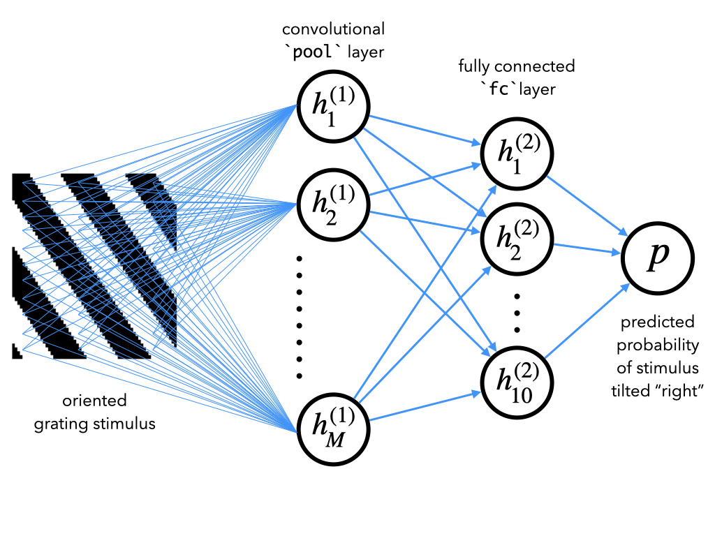
上記の方位識別課題を解くモデルを構築します。モデルは刺激画像を入力として受け取り、その刺激が右に傾いている確率を出力します。

これには、チュートリアル2で見た**畳み込みニューラルネットワーク（CNN）**を使用します。ここでは、刺激の1次元カテゴリ表現ではなく、生の刺激画像（2Dピクセル行列）に対して2次元畳み込みを行うCNNを使います。CNNは画像処理で一般的に用いられます。

今回使うCNNは2層構成です：

画像にフィルター群を畳み込む畳み込み層
畳み込みの出力を10次元表現に変換する全結合層

最後に、10次元表現を単一のスカラー $p$ に変換する出力重みがあり、これは入力刺激が右に傾いている予測確率を表します。

PyTorchでこのようなネットワークを実装する詳細はボーナスセクション1を参照してください。ここでは詳細は省き、CNNと呼ばれるこのネットワークの訓練と内部表現の解析に集中します。

次のセルを実行すると、この課題を解くためのネットワークの訓練が始まります。CNNモデルを初期化後、訓練用の方位縞刺激データセットを構築し、train()関数に渡してSGDでパラメータを最適化します。train()関数はチュートリアル1で書いたものと似た引数を取ります。

訓練完了まで約30秒かかる場合があります。

help(train)

# Set random seeds for reproducibility
np.random.seed(12)
torch.manual_seed(12)

# Initialize CNN model
net = CNN(h, w)

# Build training set to train it on
n_train = 1000  # size of training set

# sample n_train random orientations between -90 and +90 degrees
ori = (np.random.rand(n_train) - 0.5) * 180

# build orientated grating stimuli
stimuli = torch.stack([grating(i) for i in ori])

# stimulus tilt: 1. if tilted right, 0. if tilted left, as a column vector
tilt = torch.tensor(ori > 0).type(torch.float).unsqueeze(-1)

# Train model
train(net, stimuli, tilt)

セクション1.3: データの読み込み

チュートリアル開始からここまでの推定所要時間: 15分

次のセルでは、Stringer et al., 2021 のデータを読み込みます。これはマウス一次視覚野の約2万ニューロンの縞刺激に対する応答で、チュートリアル1でも使用したものです。データは以下の2つの変数に格納されています：

resp_v1 は各行が単一刺激に対する全ニューロンの応答を含む行列
ori は各刺激の方位角（度単位）を格納したベクトル。上記の規約に従い、負の角度は左傾き、正の角度は右傾きを示します。

次に、同じ刺激（oriの方位を持つ縞刺激）を深層CNNモデルに入力し、 $get_hidden_activity()$ ヘルパー関数を使ってモデルの内部表現を抽出します。この関数の出力はPythonのdictで、layer_labels引数で指定した各層の集団応答行列（resp_v1と同様）を含みます。注目するのは：

モデルの最初の畳み込み層の出力で、モデル内では'pool'として保存されているもの（なぜこの名前かはボーナスセクション1のCNN構造を参照）
全結合層の10次元出力で、モデル内では'fc'として保存されているもの

# Load mouse V1 data
resp_v1, ori = load_data(fname)

# Extract model internal representations of each stimulus in the V1 data
# construct grating stimuli for each orientation presented in the V1 data
stimuli = torch.stack([grating(a.item()) for a in ori])
layer_labels = ['pool', 'fc']
resp_model = get_hidden_activity(net, stimuli, layer_labels)

# Aggregate all responses into one dict
resp_dict = {}
resp_dict['V1 data'] = resp_v1
for k, v in resp_model.items():
  label = f"model\n'{k}' layer"
  resp_dict[label] = v

セクション2: CNNと神経活動の定量的比較

チュートリアル開始からここまでの推定所要時間: 20分

ここからは、方位識別の深層CNNモデルの内部表現を解析し、マウス一次視覚野の集団応答と比較します。

このセクションでは、CNNと一次視覚野の表現を定量的に比較します。次のセクションでは、それらの表現を可視化し構造の直感を得ます。

# @title Video 2: Quantitative comparisons of CNNs and neural activity
from ipywidgets import widgets
from IPython.display import YouTubeVideo
from IPython.display import IFrame
from IPython.display import display


class PlayVideo(IFrame):
  def __init__(self, id, source, page=1, width=400, height=300, **kwargs):
    self.id = id
    if source == 'Bilibili':
      src = f'https://player.bilibili.com/player.html?bvid={id}&page={page}'
    elif source == 'Osf':
      src = f'https://mfr.ca-1.osf.io/render?url=https://osf.io/download/{id}/?direct%26mode=render'
    super(PlayVideo, self).__init__(src, width, height, **kwargs)


def display_videos(video_ids, W=400, H=300, fs=1):
  tab_contents = []
  for i, video_id in enumerate(video_ids):
    out = widgets.Output()
    with out:
      if video_ids[i][0] == 'Youtube':
        video = YouTubeVideo(id=video_ids[i][1], width=W,
                             height=H, fs=fs, rel=0)
        print(f'Video available at https://youtube.com/watch?v={video.id}')
      else:
        video = PlayVideo(id=video_ids[i][1], source=video_ids[i][0], width=W,
                          height=H, fs=fs, autoplay=False)
        if video_ids[i][0] == 'Bilibili':
          print(f'Video available at https://www.bilibili.com/video/{video.id}')
        elif video_ids[i][0] == 'Osf':
          print(f'Video available at https://osf.io/{video.id}')
      display(video)
    tab_contents.append(out)
  return tab_contents


video_ids = [('Youtube', '2Jbk7jFBvbU'), ('Bilibili', 'BV1KT4y1j7nn')]
tab_contents = display_videos(video_ids, W=854, H=480)
tabs = widgets.Tab()
tabs.children = tab_contents
for i in range(len(tab_contents)):
  tabs.set_title(i, video_ids[i][0])
display(tabs)

# @title Submit your feedback
content_review(f"{feedback_prefix}_Quantitative_comparisons_of_CNNs_and_neural_activity_Video")

上記で、マウス一次視覚野の集団応答とモデルの異なる層の応答に類似点と相違点があることに気づきました。ここでそれを定量化してみましょう。

これには表現類似性解析（Representational Similarity Analysis）$という手法を使います。これは異なる刺激の表現間の類似構造を調べる方法です。脳の領域とモデルが似た表現スキームを使っているとは、脳で似ている（または異なる）刺激がモデルでも似ている（または異なる）ように表現されている場合に言えます。

セクション2.1: 表現非類似性行列（RDM）

これを定量化するため、マウスV1データと各モデル層の**表現非類似性行列（RDM）**を計算します。この行列を $\mathbf{M}$ と呼び、各刺激に対する集団応答間の相関係数から1を引いた値で計算します。 $z$ スコア正規化した応答を用いることで効率的に計算できます。

刺激 $s$ に対する全ニューロンの $z$ スコア応答 $\mathbf{z}^{(s)}$ は、ニューロン $i$ にわたって平均を引き、標準偏差1に正規化したものです。ニューロン数を $N$ とすると：

\mathbf{z}^{(s)} = \frac{\mathbf{r}^{(s)} - \mu^{(s)}} {\sigma^{(s)}}

ここで $\mu^{(s)} = \frac{1}{N}\sum_{i=1}^N r_i^{(s)}$ および
$\sigma^{(s)} = \sqrt{\frac{1}{N}\sum_{i=1}^N \left( r_i^{(s)} - \mu^{(s)} \right)^2}$ です。

全行列は次のように計算されます：

\mathbf{M} = 1 - \frac{1}{N} \mathbf{ZZ}^\top \\

ここで $\mathbf{Z}$ は $z$ スコア正規化された応答行列で、行は $\mathbf{r}^{(s)}$ であり、 $N$ はニューロン（またはユニット）の数です。詳細はボーナスセクション3を参照してください。

コーディング演習 2.1: RDMの計算

刺激ごとの集団応答からRDMを計算する関数 RDM() を完成させてください。上記の $z$ スコア正規化応答を用いた式を使います。 $z$ スコア応答行列の計算にはヘルパー関数 zscore() を使います。

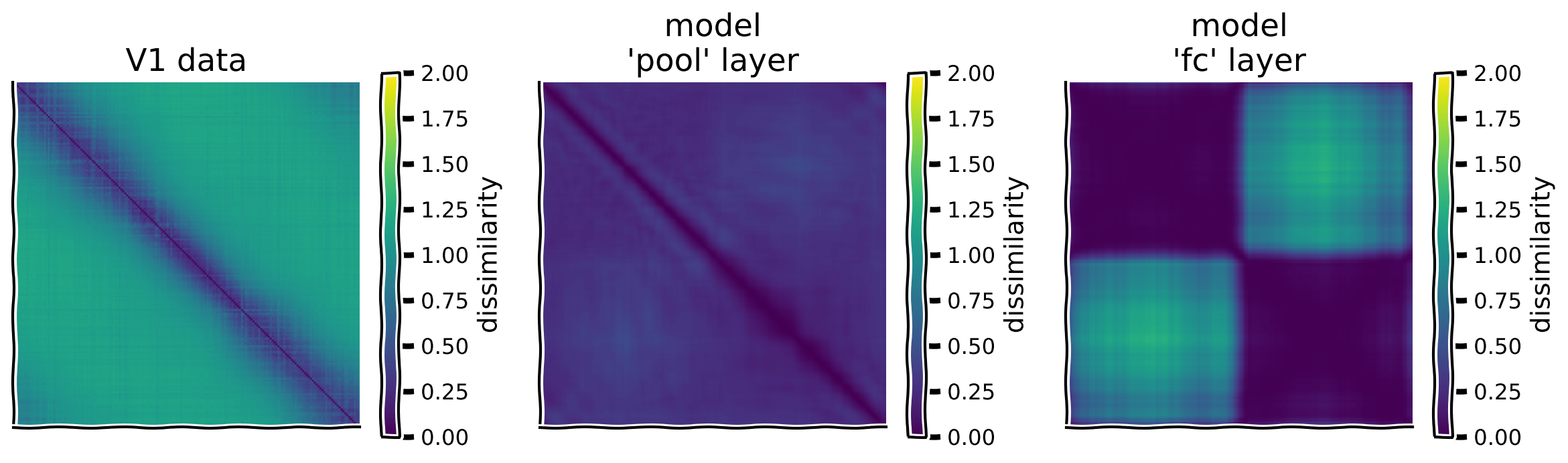
次のセルでは、この関数を使ってV1データとモデルCNNの各層の集団応答のRDMをプロットします。

def RDM(resp):
  """Compute the representational dissimilarity matrix (RDM)

  Args:
    resp (ndarray): S x N matrix with population responses to
      each stimulus in each row

  Returns:
    ndarray: S x S representational dissimilarity matrix
  """
  #########################################################
  ## TO DO for students: compute representational dissimilarity matrix
  # Fill out function and remove
  raise NotImplementedError("Student exercise: complete function RDM")
  #########################################################

  # z-score responses to each stimulus
  zresp = zscore(resp, axis=1)

  # Compute RDM
  RDM = ...

  return RDM


# Compute RDMs for each layer
rdm_dict = {label: RDM(resp) for label, resp in resp_dict.items()}

# Plot RDMs
plot_multiple_rdm(rdm_dict)

解答を見る$

出力例:

# @title Submit your feedback
content_review(f"{feedback_prefix}_Compute_RDMs_Exercise")

# @title Video 3: Coding Exercise 2.1 solution discussion
from ipywidgets import widgets
from IPython.display import YouTubeVideo
from IPython.display import IFrame
from IPython.display import display


class PlayVideo(IFrame):
  def __init__(self, id, source, page=1, width=400, height=300, **kwargs):
    self.id = id
    if source == 'Bilibili':
      src = f'https://player.bilibili.com/player.html?bvid={id}&page={page}'
    elif source == 'Osf':
      src = f'https://mfr.ca-1.osf.io/render?url=https://osf.io/download/{id}/?direct%26mode=render'
    super(PlayVideo, self).__init__(src, width, height, **kwargs)


def display_videos(video_ids, W=400, H=300, fs=1):
  tab_contents = []
  for i, video_id in enumerate(video_ids):
    out = widgets.Output()
    with out:
      if video_ids[i][0] == 'Youtube':
        video = YouTubeVideo(id=video_ids[i][1], width=W,
                             height=H, fs=fs, rel=0)
        print(f'Video available at https://youtube.com/watch?v={video.id}')
      else:
        video = PlayVideo(id=video_ids[i][1], source=video_ids[i][0], width=W,
                          height=H, fs=fs, autoplay=False)
        if video_ids[i][0] == 'Bilibili':
          print(f'Video available at https://www.bilibili.com/video/{video.id}')
        elif video_ids[i][0] == 'Osf':
          print(f'Video available at https://osf.io/{video.id}')
      display(video)
    tab_contents.append(out)
  return tab_contents


video_ids = [('Youtube', 'otzR-KXDjus'), ('Bilibili', 'BV16a4y1a7nc')]
tab_contents = display_videos(video_ids, W=854, H=480)
tabs = widgets.Tab()
tabs.children = tab_contents
for i in range(len(tab_contents)):
  tabs.set_title(i, video_ids[i][0])
display(tabs)

# @title Submit your feedback
content_review(f"{feedback_prefix}_Solution_Discussion_Video")

セクション2.2: 表現類似度の決定

チュートリアル開始からここまでの推定所要時間: 35分

表現の類似度を定量化するために、非類似性行列同士の相関係数を計算します。ここでも相関係数を使います。非類似性行列は対称行列 ( $M_{ss'} = M_{s's}$ ) なので、相関計算時には対角線の片側の非対角要素のみを使い、過剰カウントを避けます。また、対角成分は常に0であり、どのRDM間でも完全に相関するため除外します。

コーディング演習 2.2: RDMの相関計算

以下の関数 $correlate_rdms()$ を完成させてください。この関数は2つのRDM間の相関を計算します。非対角成分の抽出コードは提供しています。

この関数を使って、モデルCNNの各層のRDMとV1データのRDMの相関を計算します。

def correlate_rdms(rdm1, rdm2):
  """Correlate off-diagonal elements of two RDM's

  Args:
    rdm1 (np.ndarray): S x S representational dissimilarity matrix
    rdm2 (np.ndarray): S x S representational dissimilarity matrix to
      correlate with rdm1

  Returns:
    float: correlation coefficient between the off-diagonal elements
      of rdm1 and rdm2

  """

  # Extract off-diagonal elements of each RDM
  ioffdiag = np.triu_indices(rdm1.shape[0], k=1)  # indices of off-diagonal elements
  rdm1_offdiag = rdm1[ioffdiag]
  rdm2_offdiag = rdm2[ioffdiag]

  #########################################################
  ## TO DO for students: compute correlation coefficient
  # Fill out function and remove
  raise NotImplementedError("Student exercise: complete correlate rdms")
  #########################################################
  corr_coef = np.corrcoef(..., ...)[0,1]

  return corr_coef


# Split RDMs into V1 responses and model responses
rdm_model = rdm_dict.copy()
rdm_v1 = rdm_model.pop('V1 data')

# Correlate off-diagonal terms of dissimilarity matrices
rdm_sim = {label: correlate_rdms(rdm_v1, rdm) for label, rdm in rdm_model.items()}

# Visualize
plot_rdm_rdm_correlations(rdm_sim)

解答を見る$

出力例:

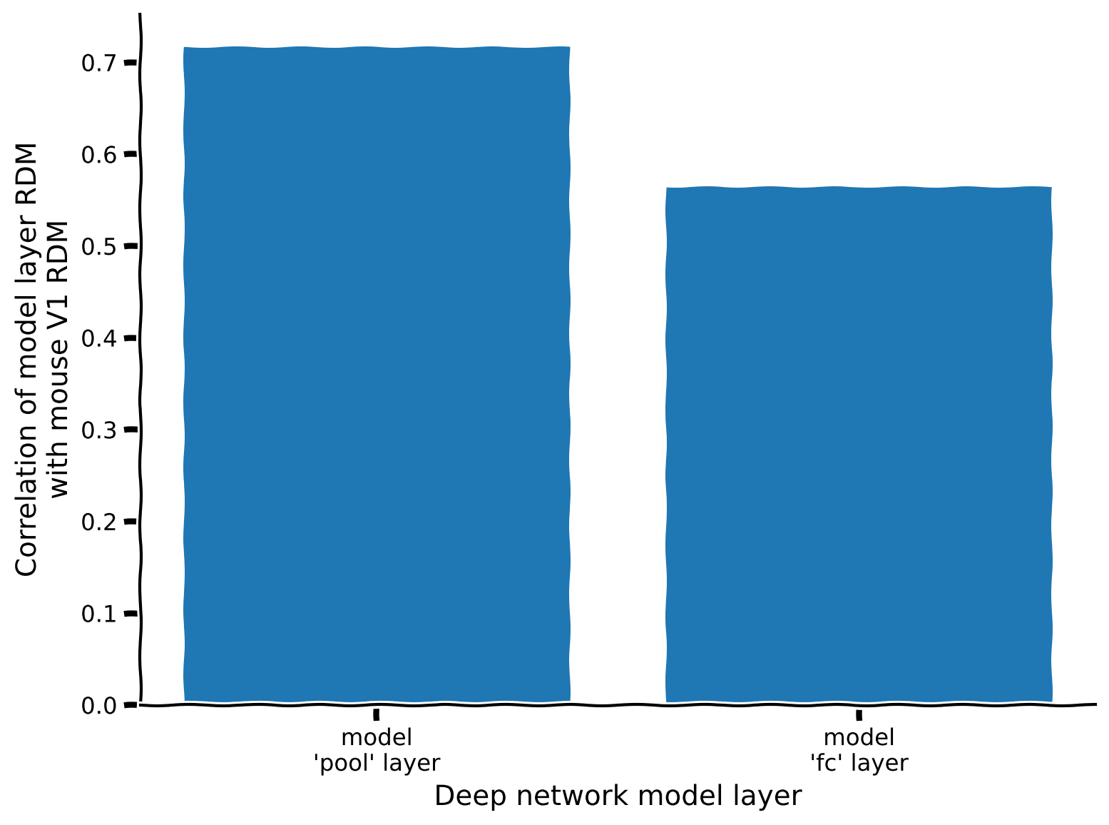
この指標によると、どの層の表現がデータの表現に最も似ていますか？コーディング演習2.1の直感と一致していますか？

# @title Submit your feedback
content_review(f"{feedback_prefix}_Correlate_RDMs_Exercise")

セクション 2.3: RDMのさらなる理解

チュートリアル開始からここまでの推定所要時間: 45分

RDMの相関がどのように生じるかをよりよく理解するために、RDM行列の個々の行をプロットしてみましょう。得られる曲線は、各刺激に対する応答と特定の1つの刺激に対する応答の類似度を示します。

ori_list = [-75, -25, 25, 75]
plot_rdm_rows(ori_list, rdm_dict, ori.numpy())

セクション 3: CNNと神経活動の定性的比較

データおよび各モデル層の表現を可視化するために、システム神経科学の古典的な2つの手法を使います：

チューニングカーブ：単一ニューロン（または深層ネットワークの場合はユニット）の刺激方向に対する応答をプロットする
次元削減：次元削減を用いて各刺激に対する全集団応答を2次元でプロットする。ここでは非線形次元削減手法のt-SNEを使用します。ユニット数が多く一度に全てを可視化するのが難しいため次元削減を用います。非線形手法を使うのは、刺激間の複雑な関係性を捉えられるためです（詳細はW1D5を参照）。

セクション 3.1: チューニングカーブ

チュートリアル開始からここまでの推定所要時間: 50分

以下に、上で訓練したCNNの異なるニューロンやユニットのチューニングカーブの例を示します。モデルとデータの単一ニューロン応答はどのように似ている/異なっているでしょうか？このセルを何度か実行して、各集団内のニューロンのチューニングカーブに共通する性質を把握してみてください。

# @markdown Execute this cell to visualize tuning curves

fig, axs = plt.subplots(1, len(resp_dict), figsize=(len(resp_dict) * 4, 4))

for i, (label, resp) in enumerate(resp_dict.items()):

  ax = axs[i]
  ax.set_title(f'{label} responses')

  # Pick three random neurons whose tuning curves to plot
  ineurons = np.random.choice(resp.shape[1], 3, replace=False)

  # Plot tuning curves of ineurons
  ax.plot(ori, resp[:, ineurons])

  ax.set_xticks(np.linspace(-90, 90, 5))
  ax.set_xlabel('stimulus orientation')
  ax.set_ylabel('neural response')

plt.tight_layout()
plt.show()

セクション 3.2: 表現の次元削減

チュートリアル開始からここまでの推定所要時間: 55分

マウス一次視覚野やCNN内部表現の次元削減版を可視化することで、有益な構造を明らかにできる可能性があります。ここではPCAで次元を20次元に削減し、その後t-SNEでさらに2次元に削減します。PCAの最初のステップを使うのはt-SNEの計算を高速化するためで、これは分野での標準的な手法です。

# @markdown Execute this cell to visualize low-d representations
def plot_resp_lowd(resp_dict):
  """Plot a low-dimensional representation of each dataset in resp_dict."""
  n_col = len(resp_dict)
  fig, axs = plt.subplots(1, n_col, figsize=(4.5 * len(resp_dict), 4.5))
  for i, (label, resp) in enumerate(resp_dict.items()):

    ax = axs[i]
    ax.set_title(f'{label} responses')

    # First do PCA to reduce dimensionality to 20 dimensions so that tSNE is faster
    resp_lowd = PCA(n_components=min(20, resp.shape[1]), random_state=0).fit_transform(resp)

    # Then do tSNE to reduce dimensionality to 2 dimensions
    resp_lowd = TSNE(n_components=2, random_state=0).fit_transform(resp_lowd)

    # Plot dimensionality-reduced population responses 'resp_lowd'
    # on 2D axes, with each point colored by stimulus orientation
    x, y = resp_lowd[:, 0], resp_lowd[:, 1]
    pts = ax.scatter(x, y, c=ori, cmap='twilight', vmin=-90, vmax=90)
    fig.colorbar(pts, ax=ax, ticks=np.linspace(-90, 90, 5),
                 label='Stimulus orientation')

    ax.set_xlabel('Dimension 1')
    ax.set_ylabel('Dimension 2')
    ax.set_xticks([])
    ax.set_yticks([])
  plt.show()


plot_resp_lowd(resp_dict)

考えてみよう！3.2: 次元削減表現の可視化

上の図を解釈してください。なぜこれらの表現はこのような形をしているのでしょうか？以下の具体的な問いを考えてみましょう：

モデルとデータの集団応答はどのように似ている/異なっているか？これらの集団レベルの応答は、前の演習で見た単一ニューロン応答から説明できるか、あるいはその逆はどうか？
モデルの異なる層の表現はどのように異なり、これはモデルが最適化された方向識別課題とどのように関連しているか？
我々の深層ネットワークのどの層の符号化モデルがV1データに最も近いか？

解答を見る$

# @title Submit your feedback
content_review(f"{feedback_prefix}_Vizualizing_reduced_dimensionality_representations_Discussion")

まとめ

チュートリアルの推定所要時間: 1時間10分

このノートブックでは以下を学びました

深層学習を用いて視覚系の規範的符号化モデルを構築する方法
RSAを用いてモデルの表現が脳内の表現とどのように一致するか評価する方法

我々のアプローチは、方向識別課題を解くために深層畳み込みネットワークを最適化することでした。しかし、他にも多くのアプローチが考えられます。

まず、方向識別課題を解く「規範的」な方法は他にも多数あります。異なるニューラルネットワークアーキテクチャを使ったり、ニューラルネットワークを使わずにフーリエ変換などの他の画像変換を用いる全く異なるアルゴリズムを使うことも可能です。しかしニューラルネットワークのアプローチは、抽象的な分散表現を用いて計算を行うため、脳が使うアルゴリズムにより近い感覚があります。特に畳み込みニューラルネットワークは視覚系の規範的モデル構築に適しています。

次に、我々の選んだ視覚課題はほぼ任意でした。例えば、単に2つの傾きクラスを識別するのではなく、刺激の方向を直接推定するようネットワークを訓練することもできます。また、任意の画像の回転を認識するなど、より自然な課題を訓練することも可能です。あるいは物体認識のような課題も考えられます。これはマウスの視覚野で計算されていることでしょうか？

異なる課題で訓練すると、傾斜格子刺激の表現が異なり、観察されたV1表現とより良く一致するかもしれませんし、逆に悪くなるかもしれません。

ボーナスチュートリアルのセクション3では、畳み込みニューラルネットワークを神経活動に直接フィットさせて符号化モデルを構築する方法を解説しています。

ボーナス

ボーナスセクション1: PyTorchでCNNを構築する

ここではPyTorchを使ってCNNの各種レイヤーを構築する手順を説明し、最終的に上で使ったCNNモデルを作ります。

ボーナスセクション1.1: 全結合層

全結合層では、各ユニットがすべての入力ユニットに対して重み付き和を計算し、この重み付き和に非線形関数を適用します。パート1と2で何度も使ったことがあるでしょう。PyTorchではnn.Linearクラスで実装されています。

次のセルには、入力画像が左または右に傾いているかを分類する1層の全結合ネットワークのコードがあります。具体的には、入力画像が右に傾いている確率を出力します。出力を確率（0から1の範囲）にするために、シグモイド活性化関数（torch.sigmoid()で実装）を使って出力を圧縮しています。

class FC(nn.Module):
  """Deep network with one fully connected layer

    Args:
      h_in (int): height of input image, in pixels (i.e. number of rows)
      w_in (int): width of input image, in pixels (i.e. number of columns)

    Attributes:
      fc (nn.Linear): weights and biases of fully connected layer
      out (nn.Linear): weights and biases of output layer

    """

  def __init__(self, h_in, w_in):
    super().__init__()
    self.dims = h_in * w_in  # dimensions of flattened input
    self.fc = nn.Linear(self.dims, 10)  # flattened input image --> 10D representation
    self.out = nn.Linear(10, 1)  # 10D representation --> scalar

  def forward(self, x):
    """Classify grating stimulus as tilted right or left

    Args:
      x (torch.Tensor): p x 48 x 64 tensor with pixel grayscale values for
          each of p stimulus images.

    Returns:
      torch.Tensor: p x 1 tensor with network outputs for each input provided
          in x. Each output should be interpreted as the probability of the
          corresponding stimulus being tilted right.

    """
    x = x.view(-1, self.dims)  # flatten each input image into a vector
    x = torch.relu(self.fc(x))  # output of fully connected layer
    x = torch.sigmoid(self.out(x))  # network output
    return x

ボーナスセクション1.2: 畳み込み層

畳み込み層では、各ユニットが2次元の $K \times K$ パッチの入力に対して重み付き和を計算します。パート2で見たように、ユニットはチャネルに配置されており（下図参照）、同じチャネル内のユニットは異なる入力領域に対して同じ重み（そのチャネルの畳み込みフィルター（カーネル））を使って重み付き和を計算します。畳み込み層の出力は形状 $C^{out} \times H \times W$ の3次元テンソルで、 $C^{out}$ はチャネル数（畳み込みフィルター数）、 $H$ と $W$ は入力の高さと幅です。

このような層はPythonでPyTorchのnn.Conv2dクラスを使って実装できます（チュートリアル2で見た、ドキュメントはこちら）。

次のセルには、上の全結合ネットワークに5 $\times$ 5サイズの畳み込みフィルター8個を持つ畳み込み層を組み込むコードがあります。畳み込み層の多チャネル出力を全結合層に渡すためにフラット化する必要があることに注意してください。

class ConvFC(nn.Module):
  """Deep network with one convolutional layer and one fully connected layer

  Args:
    h_in (int): height of input image, in pixels (i.e. number of rows)
    w_in (int): width of input image, in pixels (i.e. number of columns)

  Attributes:
    conv (nn.Conv2d): filter weights of convolutional layer
    dims (tuple of ints): dimensions of output from conv layer
    fc (nn.Linear): weights and biases of fully connected layer
    out (nn.Linear): weights and biases of output layer

  """

  def __init__(self, h_in, w_in):
    super().__init__()
    C_in = 1  # input stimuli have only 1 input channel
    C_out = 6  # number of output channels (i.e. of convolutional kernels to convolve the input with)
    K = 7  # size of each convolutional kernel (should be odd number for the padding to work as expected)
    self.conv = nn.Conv2d(C_in, C_out, kernel_size=K, padding=K//2)  # add padding to ensure that each channel has same dimensionality as input
    self.dims = (C_out, h_in, w_in)  # dimensions of conv layer output
    self.fc = nn.Linear(np.prod(self.dims), 10)  # flattened conv output --> 10D representation
    self.out = nn.Linear(10, 1)  # 10D representation --> scalar

  def forward(self, x):
    """Classify grating stimulus as tilted right or left

    Args:
      x (torch.Tensor): p x 48 x 64 tensor with pixel grayscale values for
          each of p stimulus images.

    Returns:
      torch.Tensor: p x 1 tensor with network outputs for each input provided
          in x. Each output should be interpreted as the probability of the
          corresponding stimulus being tilted right.

    """
    x = x.unsqueeze(1)  # p x 1 x 48 x 64, add a singleton dimension for the single stimulus channel
    x = torch.relu(self.conv(x))  # output of convolutional layer
    x = x.view(-1, np.prod(self.dims))  # flatten convolutional layer outputs into a vector
    x = torch.relu(self.fc(x))  # output of fully connected layer
    x = torch.sigmoid(self.out(x))  # network output
    return x

ボーナスセクション1.3: マックスプーリング層

マックスプーリング層では、各ユニットが小さな2次元の $K^{pool} \times K^{pool}$ パッチの入力の最大値を計算します。多チャネル入力の次元が $C \times H \times W$ の場合、マックスプーリング層の出力の次元は $C \times H^{out} \times W^{out}$ で、

\begin{align}
$H^{out}$ &= $\left\lfloor \frac{H}{K^{pool}} \right\rfloor$ \
$W^{out}$ &= $\left\lfloor \frac{W}{K^{pool}} \right\rfloor \end{align}$

ここで $\lfloor\cdot\rfloor$ は小数点以下切り捨て（Pythonの//演算子）を意味します。

マックスプーリング層はPyTorchのnn.MaxPool2dクラスで実装でき、プーリングパッチのサイズ $K^{pool}$ を引数に取ります。次のセルには、畳み込み層の直後にマックスプーリング層を追加した例があります。出力の次元を計算して、次の全結合層の入力次元を設定する必要があることに注意してください。

class ConvPoolFC(nn.Module):
  """Deep network with one convolutional layer followed by a max pooling layer
  and one fully connected layer

  Args:
    h_in (int): height of input image, in pixels (i.e. number of rows)
    w_in (int): width of input image, in pixels (i.e. number of columns)

  Attributes:
    conv (nn.Conv2d): filter weights of convolutional layer
    pool (nn.MaxPool2d): max pooling layer
    dims (tuple of ints): dimensions of output from pool layer
    fc (nn.Linear): weights and biases of fully connected layer
    out (nn.Linear): weights and biases of output layer

  """

  def __init__(self, h_in, w_in):
    super().__init__()
    C_in = 1  # input stimuli have only 1 input channel
    C_out = 6  # number of output channels (i.e. of convolutional kernels to convolve the input with)
    K = 7  # size of each convolutional kernel
    Kpool = 8  # size of patches over which to pool
    self.conv = nn.Conv2d(C_in, C_out, kernel_size=K, padding=K//2)  # add padding to ensure that each channel has same dimensionality as input
    self.pool = nn.MaxPool2d(Kpool)
    self.dims = (C_out, h_in // Kpool, w_in // Kpool)  # dimensions of pool layer output
    self.fc = nn.Linear(np.prod(self.dims), 10)  # flattened pool output --> 10D representation
    self.out = nn.Linear(10, 1)  # 10D representation --> scalar

  def forward(self, x):
    """Classify grating stimulus as tilted right or left

    Args:
      x (torch.Tensor): p x 48 x 64 tensor with pixel grayscale values for
          each of p stimulus images.

    Returns:
      torch.Tensor: p x 1 tensor with network outputs for each input provided
          in x. Each output should be interpreted as the probability of the
          corresponding stimulus being tilted right.

    """
    x = x.unsqueeze(1)  # p x 1 x 48 x 64, add a singleton dimension for the single stimulus channel
    x = torch.relu(self.conv(x))  # output of convolutional layer
    x = self.pool(x)  # output of pooling layer
    x = x.view(-1, np.prod(self.dims))  # flatten pooling layer outputs into a vector
    x = torch.relu(self.fc(x))  # output of fully connected layer
    x = torch.sigmoid(self.out(x))  # network output
    return x

このプーリング層は、上で訓練した方向識別を行うCNNモデルを完成させます。このアーキテクチャは主に2つの層から成り立っています：

畳み込み＋プーリング層
全結合層

畳み込み層とプーリング層は1つの処理単位としてまとめられます。画像の各パッチが畳み込みフィルターを通り、隣接パッチとプーリングされるためです。畳み込み層の後にプーリング層を置くのは標準的な手法であり、通常は1つの処理ブロックとして扱われます。

ボーナスセクション2: 方向識別を二値分類問題として扱う

方向識別課題の性能を最適化するために最小化すべき損失関数は何でしょうか？まず、方向識別課題は二値分類問題であり、刺激を左傾きか右傾きのいずれかのクラスに分類することが目的です。

したがって、刺激が右に傾いているときは右に傾いている確率（ $p$ ）を高く出力し、左に傾いているときは左に傾いている確率（ $1-p$ ）を高く出力することが目標です。

ミニバッチ内の $n$ 番目の刺激の真の傾きを示すラベルを $\tilde{y}^{(n)}$ とします：

\tilde{y}^{(n)} = \begin{cases} 1 &\text{刺激 } n \text{ が右に傾いている場合} \\ 0 &\text{刺激 } n \text{ が左に傾いている場合} \end{cases}

ネットワークが予測したその刺激が右に傾いている確率を $p^{(n)}$ とします。 $1-p^{(n)}$ は左に傾いている確率です。パラメータを調整して真のクラス $\tilde{y}^{(n)}$ の予測確率を最大化したいです。これを形式化すると、対数確率を最大化することになります：

\begin{align}
$\log \left( \text{刺激 } n \text{ がクラス } \tilde{y}^{(n)} \text{ である予測確率} \right)$ &=
\begin{cases}
$\log p^{(n)}$ & $\text{if }\tilde{y}^{(n)} = 1$ \
$\log (1 - p^{(n)})$ & $\text{if }\tilde{y}^{(n)} = 0 \end{cases}$
\
&= $\tilde{y}^{(n)} \log p^{(n)} + (1 - \tilde{y}^{(n)})\log(1 - p^{(n)}) \end{align}$

この式はベルヌーイ分布の対数尤度であることに気づくでしょう。これはロジスティック回帰で最大化される量と同じで、ロジスティック回帰では予測確率 $p^{(n)}$ は入力の単純な線形和ですが、ここでは深層ネットワークのような複雑な非線形演算です。

これを損失関数に変えるには-1をかけて、二値交差エントロピーまたは負の対数尤度と呼ばれるものにします。バッチ内の $P$ サンプルで和を取ると、二値交差エントロピー損失は

L = -\sum_{n=1}^P \tilde{y}^{(n)} \log p^{(n)} + (1 - \tilde{y}^{(n)})\log(1 - p^{(n)})

PyTorchではnn.BCELoss()損失関数で実装できます（ドキュメント）。

ノートブック上部のヘルパー関数の隠しセルにあるtrain()関数でCNNの最適化に使われているコードもぜひ確認してください。ここで使うCNNはパラメータが多いため、前のパートで使わなかった2つの工夫が必要です：

勾配降下法（GD）ではなく確率的勾配降下法（SGD）を使う
SGDの更新にモーメンタムを使う。PyTorchのoptim.SGDのmomentum引数を設定するだけで簡単に組み込めます。

ボーナスセクション3: RDMのZスコア説明

$i$ 番目のニューロンの $s$ 番目の刺激に対する応答を $r^{(s)}_i$ とすると、

\begin{gather}
$M_{ss$ '} = 1 - $\frac{\text{Cov}\left$ [ $r_i^{(s)},$ $r_i^{(s$ ')} $\right$ ]}{ $\sqrt{\text{Var}\left$ [ $r_i^{(s)}$ $\right$ ] $\text{Var}\left$ [ $r_i^{(s$ ')} $\right$ ]}} = 1 - $\frac{\sum_{i=1}^N (r_i^{(s)} - \bar{r}^{(s)})(r_i^{(s')} - \bar{r}^{(s')}) }{\sqrt{\sum_{i=1}^N \left( r_i^{(s)} - \bar{r}^{(s)} \right)^2 \sum_{i=1}^N \left( r_i^{(s')} - \bar{r}^{(s')} \right)^2 }}$ \
$\bar{r}^{(s)} = \frac{1}{N} \sum_{i=1}^N r_i^{(s)} \end{gather}$

これは $z$ スコア化された応答を使うことで効率的に計算できます。

z_i^{(s)} = \frac{r_i^{(s)} - \bar{r}^{(s)}}{\sqrt{\frac{1}{N}\sum_{i=1}^N \left( r_i^{(s)} - \bar{r}^{(s)} \right)^2}} \Rightarrow M_{ss'} = 1 - \frac{1}{N}\sum_{i=1}^N z_i^{(s)}z_i^{(s')}

このようにして、行列積で全体の行列を計算できます。
\begin{gather}
$\mathbf{M} = 1 - \frac{1}{N} \mathbf{ZZ}^\top$ \
$\mathbf{Z} = \begin{bmatrix} z_1^{(1)}$ & $z_2^{(1)}$ & $\ldots$ & $z_N^{(1)}$ \
$z_1^{(2)}$ & $z_2^{(2)}$ & $\ldots$ & $z_N^{(2)}$ \
$\vdots$ & $\vdots$ & $\ddots$ & $\vdots$ \
$z_1^{(S)}$ & $z_2^{(S)}$ & $\ldots$ & $z_N^{(S)}$
\end{bmatrix}
\end{gather}

ここで $S$ は刺激の総数です。 $\mathbf{Z}$ は $S \times N$ 行列、 $\mathbf{M}$ は $S \times S$ 行列です。