チュートリアル 2: 畳み込みニューラルネットワーク

第1週 第5日目: ディープラーニング

Neuromatch Academyによる

コンテンツ作成者: Jorge A. Menendez, Carsen Stringer

コンテンツレビュアー: Roozbeh Farhoodi, Madineh Sarvestani, Kshitij Dwivedi, Spiros Chavlis, Ella Batty, Michael Waskom

制作編集者: Spiros Chavlis

チュートリアルの目的

推定所要時間: 40分

この短いチュートリアルでは、2D畳み込みの基本を学び、チュートリアル3での規範的モデル作成に備えて画像に畳み込みネットワークを適用します。

このチュートリアルでは以下を行います。

• 2D畳み込みの基本を理解する
• PyTorchを使って畳み込み層を構築する
• その出力を可視化・解析する

# @title Tutorial slides
# @markdown These are the slides for all videos in this tutorial.
from IPython.display import IFrame
link_id = "s59jy"
print(f"If you want to download the slides: https://osf.io/download/{link_id}/")
IFrame(src=f"https://mfr.ca-1.osf.io/render?url=https://osf.io/{link_id}/?direct%26mode=render%26action=download%26mode=render", width=854, height=480)

セットアップ

# @title Install and import feedback gadget


from vibecheck import DatatopsContentReviewContainer
def content_review(notebook_section: str):
    return DatatopsContentReviewContainer(
        "",  # No text prompt
        notebook_section,
        {
            "url": "https://pmyvdlilci.execute-api.us-east-1.amazonaws.com/klab",
            "name": "neuromatch_cn",
            "user_key": "y1x3mpx5",
        },
    ).render()


feedback_prefix = "W1D5_T2"

# Imports
import os
import numpy as np
import torch
from torch import nn
from torch import optim
from matplotlib import pyplot as plt
import matplotlib as mpl

# @title Figure settings
import logging
logging.getLogger('matplotlib.font_manager').disabled = True

%matplotlib inline
%config InlineBackend.figure_format = 'retina'
plt.style.use("https://raw.githubusercontent.com/NeuromatchAcademy/course-content/main/nma.mplstyle")

# @title Plotting Functions

def show_stimulus(img, ax=None, show=False):
  """Visualize a stimulus"""
  if ax is None:
    ax = plt.gca()
  ax.imshow(img+0.5, cmap=mpl.cm.binary)
  ax.set_xticks([])
  ax.set_yticks([])
  ax.spines['left'].set_visible(False)
  ax.spines['bottom'].set_visible(False)
  if show:
    plt.show()


def plot_weights(weights, channels=[0]):
  """ plot convolutional channel weights
  Args:
      weights: weights of convolutional filters (conv_channels x K x K)
      channels: which conv channels to plot
  """
  wmax = torch.abs(weights).max()
  fig, axs = plt.subplots(1, len(channels), figsize=(12, 2.5))
  for i, channel in enumerate(channels):
    im = axs[i].imshow(weights[channel, 0], vmin=-wmax, vmax=wmax, cmap='bwr')
    axs[i].set_title(f'channel {channel}')

    cb_ax = fig.add_axes([1, 0.1, 0.05, 0.8])
    plt.colorbar(im, ax=cb_ax)
    cb_ax.axis('off')
  plt.show()


def plot_example_activations(stimuli, act, channels=[0]):
  """ plot activations act and corresponding stimulus
  Args:
    stimuli: stimulus input to convolutional layer (n x h x w) or (h x w)
    act: activations of convolutional layer (n_bins x conv_channels x n_bins)
    channels: which conv channels to plot
  """
  if stimuli.ndim>2:
    n_stimuli = stimuli.shape[0]
  else:
    stimuli = stimuli.unsqueeze(0)
    n_stimuli = 1

  fig, axs = plt.subplots(n_stimuli, 1 + len(channels), figsize=(12, 12))

  # plot stimulus
  for i in range(n_stimuli):
    show_stimulus(stimuli[i].squeeze(), ax=axs[i, 0])
    axs[i, 0].set_title('stimulus')

    # plot example activations
    for k, (channel, ax) in enumerate(zip(channels, axs[i][1:])):
      im = ax.imshow(act[i, channel], vmin=-3, vmax=3, cmap='bwr')
      ax.set_xlabel('x-pos')
      ax.set_ylabel('y-pos')
      ax.set_title(f'channel {channel}')

    cb_ax = fig.add_axes([1.05, 0.8, 0.01, 0.1])
    plt.colorbar(im, cax=cb_ax)
    cb_ax.set_title('activation\n strength')
  plt.show()

# @title Helper Functions

def load_data_split(data_name):
  """Load mouse V1 data from Stringer et al. (2019)

  Data from study reported in this preprint:
  https://www.biorxiv.org/content/10.1101/679324v2.abstract

  These data comprise time-averaged responses of ~20,000 neurons
  to ~4,000 stimulus gratings of different orientations, recorded
  through Calcium imaginge. The responses have been normalized by
  spontaneous levels of activity and then z-scored over stimuli, so
  expect negative numbers. The responses were split into train and
  test and then each set were averaged in bins of 6 degrees.

  This function returns the relevant data (neural responses and
  stimulus orientations) in a torch.Tensor of data type torch.float32
  in order to match the default data type for nn.Parameters in
  Google Colab.

  It will hold out some of the trials when averaging to allow us to have test
  tuning curves.

  Args:
    data_name (str): filename to load

  Returns:
    resp_train (torch.Tensor): n_stimuli x n_neurons matrix of neural responses,
        each row contains the responses of each neuron to a given stimulus.
        As mentioned above, neural "response" is actually an average over
        responses to stimuli with similar angles falling within specified bins.
    resp_test (torch.Tensor): n_stimuli x n_neurons matrix of neural responses,
        each row contains the responses of each neuron to a given stimulus.
        As mentioned above, neural "response" is actually an average over
        responses to stimuli with similar angles falling within specified bins
    stimuli: (torch.Tensor): n_stimuli x 1 column vector with orientation
        of each stimulus, in degrees. This is actually the mean orientation
        of all stimuli in each bin.

  """
  with np.load(data_name) as dobj:
    data = dict(**dobj)
  resp_train = data['resp_train']
  resp_test = data['resp_test']
  stimuli = data['stimuli']

  # Return as torch.Tensor
  resp_train_tensor = torch.tensor(resp_train, dtype=torch.float32)
  resp_test_tensor = torch.tensor(resp_test, dtype=torch.float32)
  stimuli_tensor = torch.tensor(stimuli, dtype=torch.float32)

  return resp_train_tensor, resp_test_tensor, stimuli_tensor


def filters(out_channels=6, K=7):
  """ make example filters, some center-surround and gabors
  Returns:
      filters: out_channels x K x K
  """
  grid = np.linspace(-K/2, K/2, K).astype(np.float32)
  xx,yy = np.meshgrid(grid, grid, indexing='ij')

  # create center-surround filters
  sigma = 1.1
  gaussian = np.exp(-(xx**2 + yy**2)**0.5/(2*sigma**2))
  wide_gaussian = np.exp(-(xx**2 + yy**2)**0.5/(2*(sigma*2)**2))
  center_surround = gaussian - 0.5 * wide_gaussian

  # create gabor filters
  thetas = np.linspace(0, 180, out_channels-2+1)[:-1] * np.pi/180
  gabors = np.zeros((len(thetas), K, K), np.float32)
  lam = 10
  phi = np.pi/2
  gaussian = np.exp(-(xx**2 + yy**2)**0.5/(2*(sigma*0.4)**2))
  for i,theta in enumerate(thetas):
    x = xx*np.cos(theta) + yy*np.sin(theta)
    gabors[i] = gaussian * np.cos(2*np.pi*x/lam + phi)

  filters = np.concatenate((center_surround[np.newaxis,:,:],
                            -1*center_surround[np.newaxis,:,:],
                            gabors),
                           axis=0)
  filters /= np.abs(filters).max(axis=(1,2))[:,np.newaxis,np.newaxis]
  filters -= filters.mean(axis=(1,2))[:,np.newaxis,np.newaxis]
  # convert to torch
  filters = torch.from_numpy(filters)
  # add channel axis
  filters = filters.unsqueeze(1)

  return filters


def grating(angle, sf=1 / 28, res=0.1, patch=False):
  """Generate oriented grating stimulus

  Args:
    angle (float): orientation of grating (angle from vertical), in degrees
    sf (float): controls spatial frequency of the grating
    res (float): resolution of image. Smaller values will make the image
      smaller in terms of pixels. res=1.0 corresponds to 640 x 480 pixels.
    patch (boolean): set to True to make the grating a localized
      patch on the left side of the image. If False, then the
      grating occupies the full image.

  Returns:
    torch.Tensor: (res * 480) x (res * 640) pixel oriented grating image

  """

  angle = np.deg2rad(angle)  # transform to radians

  wpix, hpix = 640, 480  # width and height of image in pixels for res=1.0

  xx, yy = np.meshgrid(sf * np.arange(0, wpix * res) / res, sf * np.arange(0, hpix * res) / res)

  if patch:
    gratings = np.cos(xx * np.cos(angle + .1) + yy * np.sin(angle + .1))  # phase shift to make it better fit within patch
    gratings[gratings < 0] = 0
    gratings[gratings > 0] = 1
    xcent = gratings.shape[1] * .75
    ycent = gratings.shape[0] / 2
    xxc, yyc = np.meshgrid(np.arange(0, gratings.shape[1]), np.arange(0, gratings.shape[0]))
    icirc = ((xxc - xcent) ** 2 + (yyc - ycent) ** 2) ** 0.5 < wpix / 3 / 2 * res
    gratings[~icirc] = 0.5

  else:
    gratings = np.cos(xx * np.cos(angle) + yy * np.sin(angle))
    gratings[gratings < 0] = 0
    gratings[gratings > 0] = 1

  gratings -= 0.5

  # Return torch tensor
  return torch.tensor(gratings, dtype=torch.float32)

# @title Data retrieval and loading

import hashlib
import requests

fname = "W3D4_stringer_oribinned6_split.npz"
url = "https://osf.io/p3aeb/download"
expected_md5 = "b3f7245c6221234a676b71a1f43c3bb5"

if not os.path.isfile(fname):
  try:
    r = requests.get(url)
  except requests.ConnectionError:
    print("!!! Failed to download data !!!")
  else:
    if r.status_code != requests.codes.ok:
      print("!!! Failed to download data !!!")
    elif hashlib.md5(r.content).hexdigest() != expected_md5:
      print("!!! Data download appears corrupted !!!")
    else:
      with open(fname, "wb") as fid:
        fid.write(r.content)

セクション1: 2D畳み込みの紹介

セクション1.1: 2D畳み込みとは？

2D畳み込みは、フィルター$f$と入力画像$I$の積の積分であり、フィルターを入力上でスライドさせながら様々な位置で計算されます。位置$(x,y)$での畳み込み演算の出力は、フィルター$f$のサイズが$(K, K)$の場合、次のように表されます：

この畳み込みフィルターはしばしばカーネルと呼ばれます。

こちらはこの記事からの2D畳み込みの図解です：

# @markdown Execute this cell to view convolution gif

from IPython.display import Image
Image(url='https://miro.medium.com/max/700/1*5BwZUqAqFFP5f3wKYQ6wJg.gif')

セクション1.2: ディープラーニングにおける2D畳み込み

チュートリアル開始からここまでの推定時間: 6分

# @title Video 1: 2D Convolutions
from ipywidgets import widgets
from IPython.display import YouTubeVideo
from IPython.display import IFrame
from IPython.display import display


class PlayVideo(IFrame):
  def __init__(self, id, source, page=1, width=400, height=300, **kwargs):
    self.id = id
    if source == 'Bilibili':
      src = f'https://player.bilibili.com/player.html?bvid={id}&page={page}'
    elif source == 'Osf':
      src = f'https://mfr.ca-1.osf.io/render?url=https://osf.io/download/{id}/?direct%26mode=render'
    super(PlayVideo, self).__init__(src, width, height, **kwargs)


def display_videos(video_ids, W=400, H=300, fs=1):
  tab_contents = []
  for i, video_id in enumerate(video_ids):
    out = widgets.Output()
    with out:
      if video_ids[i][0] == 'Youtube':
        video = YouTubeVideo(id=video_ids[i][1], width=W,
                             height=H, fs=fs, rel=0)
        print(f'Video available at https://youtube.com/watch?v={video.id}')
      else:
        video = PlayVideo(id=video_ids[i][1], source=video_ids[i][0], width=W,
                          height=H, fs=fs, autoplay=False)
        if video_ids[i][0] == 'Bilibili':
          print(f'Video available at https://www.bilibili.com/video/{video.id}')
        elif video_ids[i][0] == 'Osf':
          print(f'Video available at https://osf.io/{video.id}')
      display(video)
    tab_contents.append(out)
  return tab_contents


video_ids = [('Youtube', 'zgO9rHYbDxE'), ('Bilibili', 'BV1jw411d7Kg')]
tab_contents = display_videos(video_ids, W=854, H=480)
tabs = widgets.Tab()
tabs.children = tab_contents
for i in range(len(tab_contents)):
  tabs.set_title(i, video_ids[i][0])
display(tabs)

# @title Submit your feedback
content_review(f"{feedback_prefix}_2D_Convolutions_Video")

この動画では畳み込みの説明とPyTorchでの実装方法を解説しています。

物体認識は、深層畳み込みニューラルネットワークを効果的に訓練する技術の登場まで、機械学習においてほぼ未解決の問題でした。視覚系をモデル化するためにCNNを使う理由についてはボーナスセクション1を参照してください。

畳み込みニューラルネットワークは2D畳み込み層、ReLU非線形性、2Dプーリング層、そして出力に全結合層を含みます。これらすべての要素を含む例をチュートリアル3で見ます。

2D畳み込み層は複数の出力チャネルを持ちます。各出力チャネルは入力に適用された2D畳み込みフィルターの結果です。下のGIFでは、入力が青、フィルターが灰色、出力が緑で示されています。出力チャネルのユニット数は設定したストライドによります。下のGIFではストライドは1で、入力画像の各位置でサンプリングしています。ストライド2なら入力位置を飛ばします。ほとんどの応用、特に小さなフィルターサイズではストライド1が使われます。

（技術的注記：フィルターサイズKが奇数で、pad=K//2、stride=1（下図のように）を設定すると、入力と同じサイズのチャネルが得られます。ストライドとパッドの詳細はこちら$を参照してください）。

# @markdown Execute this cell to view convolution gif

from IPython.display import Image
Image(url='https://miro.medium.com/max/790/1*1okwhewf5KCtIPaFib4XaA.gif')

セクション1.3: PyTorchにおける2D畳み込み

チュートリアル開始からここまでの推定時間: 18分

チュートリアル1では、全結合線形層を使って神経活動から刺激をデコードしました。畳み込み層は全結合層と2点で異なります：

• 全結合層では各ユニットが全入力ユニットに対して重み付き和を計算しますが、畳み込み層では各ユニットが入力の小さなパッチ（ユニットの受容野）に対してのみ重み付き和を計算します。入力が画像の場合、受容野は局所的なピクセルのパッチと考えられます。
• 全結合層では各ユニットが独立した重みセットを使いますが、畳み込み層では同じチャネル内の全ユニットが同じ重みを共有します。この共有重みセットを畳み込みフィルターまたはカーネルと呼びます。この計算の結果は畳み込みであり、各ユニットは入力の異なる部分に対して同じ重み付き和を計算します。これによりネットワークのパラメータ数が大幅に減ります。

以下のThink演習で、全結合層と畳み込み層の重み数の違いを計算します。

まず、チュートリアル1のデータセットの刺激を可視化しましょう。Stringer et al., 2021の神経記録中、マウスには向き付きグレーティングが提示されました：

# @markdown Execute this cell to plot example stimuli

orientations = np.linspace(-90, 90, 5)

h_ = 3
n_col = len(orientations)
h, w  = grating(0).shape  # height and width of stimulus

fig, axs = plt.subplots(1, n_col, figsize=(h_ * n_col, h_))
for i, ori in enumerate(orientations):
  stimulus = grating(ori)
  axs[i].set_title(f'{ori: .0f}$^o$')
  show_stimulus(stimulus, axs[i])
fig.suptitle(f'stimulus size: {h} x {w}')
plt.show()

次に2D畳み込み演算を実装します。複数の畳み込みチャネルを使い、PyTorchで効率的に実装します。畳み込みチャネルの層はPyTorchのクラスnn.Conv2d()を使って1行で実装できます。初期化には以下の引数が必要です（詳細は公式ドキュメント参照）：

• $C^{in}$: 入力チャネル数
• $C^{out}$: 出力チャネル数（異なる畳み込みフィルターの数）
• $K$: $C^{out}$個の異なる畳み込みフィルターのサイズ

ネットワークを実行するとき、任意のサイズ$(H^{in}, W^{in})$の刺激を入力できますが、形状は4Dテンソル$(N, C^{in}, H^{in}, W^{in})$である必要があります。ここで$N$は画像数です。今回$C^{in}=1$で、画像はグレースケール（多くの画像処理では$C^{in}=3$）です。

class ConvolutionalLayer(nn.Module):
  """Deep network with one convolutional layer
     Attributes: conv (nn.Conv2d): convolutional layer
  """
  def __init__(self, c_in=1, c_out=6, K=7, filters=None):
    """Initialize layer

    Args:
        c_in: number of input stimulus channels
        c_out: number of output convolutional channels
        K: size of each convolutional filter
        filters: (optional) initialize the convolutional weights

    """
    super().__init__()
    self.conv = nn.Conv2d(c_in, c_out, kernel_size=K,
                          padding=K//2, stride=1)
    if filters is not None:
      self.conv.weight = nn.Parameter(filters)
      self.conv.bias = nn.Parameter(torch.zeros((c_out,), dtype=torch.float32))

  def forward(self, s):
    """Run stimulus through convolutional layer

    Args:
        s (torch.Tensor): n_stimuli x c_in x h x w tensor with stimuli

    Returns:
        (torch.Tensor): n_stimuli x c_out x h x w tensor with convolutional layer unit activations.

    """
    a = self.conv(s)  # output of convolutional layer

    return a

ConvolutionalLayerはfiltersを入力として受け取ります。以下のfilters関数で事前に設計したフィルターを使えます。これらは網膜や視覚野の生物学的回路で実装されていると考えられるフィルターに似ています。いくつかは中心周辺フィルター、いくつかはガボールフィルターです。中心周辺フィルターの詳細はこのウェブサイト、ガボールフィルターの詳細はこのウェブサイト$を参照してください。

# @markdown Execute this cell to create and visualize filters

example_filters = filters(out_channels=6, K=7)

plt.figure(figsize=(8,4))
plt.subplot(1,2,1)
plt.imshow(example_filters[0,0], vmin=-1, vmax=1, cmap='bwr')
plt.title('center-surround filter')
plt.axis('off')
plt.subplot(1,2,2)
plt.imshow(example_filters[4,0], vmin=-1, vmax=1, cmap='bwr')
plt.title('gabor filter')
plt.axis('off')
plt.show()

コーディング演習 1.3: PyTorchでの2D畳み込み

これから畳み込み層を刺激に適用します。刺激は関数gratingで作成したグレーティング刺激で、サイズは48 x 64です。

復習ですが、nn.Conv2dはサイズ$(N, C^{in}, H^{in}, W^{in})$のテンソルを入力とします。ここで$N$は刺激数、$C^{in}$は入力チャネル数、$(H^{in}, W^{in})$は刺激のサイズです。刺激に最初の2次元を追加してから畳み込み層に入力します。

畳み込みの出力をプロットします。convoutはサイズ$(N, C^{out}, H^{in}, W^{in})$のテンソルで、$N$は例の数、$C^{out}$は畳み込みチャネル数です。ストライド1とカーネルサイズの半分のパディングを使ったため、入力と同じサイズです。

# Stimulus parameters
in_channels = 1  # how many input channels in our images
h = 48  # height of images
w = 64  # width of images

# Convolution layer parameters
K = 7  # filter size
out_channels = 6  # how many convolutional channels to have in our layer
example_filters = filters(out_channels, K)  # create filters to use

convout = np.zeros(0)  # assign convolutional activations to convout

################################################################################
## TODO for students: create convolutional layer in pytorch
# Complete and uncomment
raise NotImplementedError("Student exercise: create convolutional layer")
################################################################################

# Initialize conv layer and add weights from function filters
# you need to specify :
# * the number of input channels c_in
# * the number of output channels c_out
# * the filter size K
convLayer = ConvolutionalLayer(..., filters=example_filters)

# Create stimuli (H_in, W_in)
orientations = [-90, -45, 0, 45, 90]
stimuli = torch.zeros((len(orientations), in_channels, h, w), dtype=torch.float32)
for i,ori in enumerate(orientations):
  stimuli[i, 0] = grating(ori)

convout = convLayer(...)
convout = convout.detach()  # detach gradients

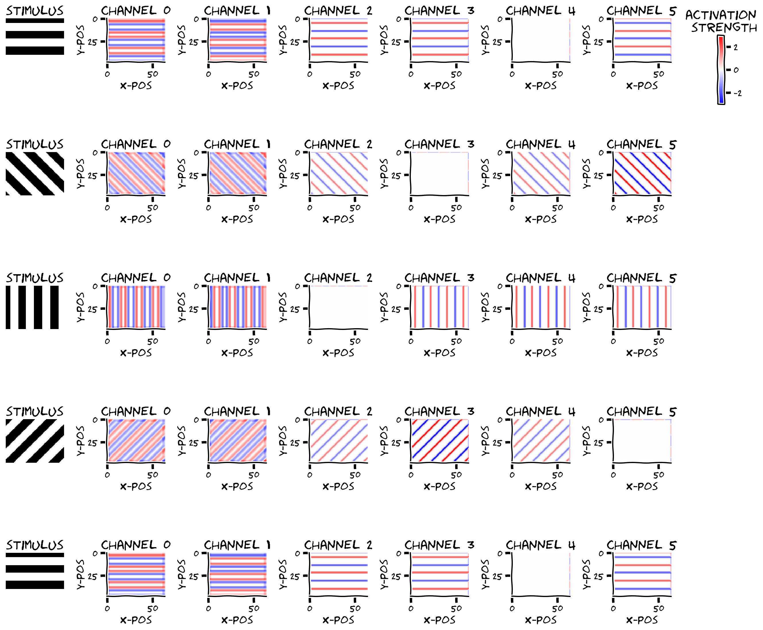
plot_example_activations(stimuli, convout, channels=np.arange(0, out_channels))

解答を見る$

出力例:

# @title Submit your feedback
content_review(f"{feedback_prefix}_2D_Convolution_in_pytorch_Exercise")

考えてみよう 1.3: 畳み込み層の出力と重みの形状

convLayerの重みと出力の形状について考えましょう：

• 各チャネルに畳み込み活性化は何個あり、なぜそのサイズなのか？
• convLayerの重みは何個あるか？
• 全結合層だったら重みは何個になるか？

さらに、活性化の見た目について考えましょう。すべてのチャネルで活性化はグレーティングのエッジ（白から黒、黒から白に変わる部分）でのみ非ゼロのようです。

• チャネル0と1は向きに関係なくすべてのエッジに反応しますが、符号が異なります。どんなフィルターがこのような応答を生むでしょう？
• チャネル2-5は刺激の向きによって異なる応答を示します。どんなフィルターがこのような応答を生むでしょう？

解答を見る$

# @title Submit your feedback
content_review(f"{feedback_prefix}_Output_and_weight_shapes_conv_layer_Discussion")

ボーナスセクション2で畳み込みフィルターの重みを可視化できます。ボーナスチュートリアルではCNNを神経のエンコーディングモデルとして使う方法（神経応答に直接フィット）を紹介しています。

まとめ

推定所要時間: 40分

このノートブックでは、マウス視覚野のニューロンの応答、あるいはマウス視覚野への入力ニューロンの応答を表すことを意図した2D畳み込み層を構築しました。

チュートリアル3では、この2D畳み込み層に全結合層を追加し、向きが左か右かを予測するモデルを訓練します。学習された畳み込みフィルターがマウス視覚野に似ているかを調べます。ボーナスチュートリアルのセクション3では、畳み込みニューラルネットワークを神経活動に直接フィットさせる方法を紹介しています。

ボーナス

ボーナスセクション1: なぜCNNなのか？

CNNモデルは視覚系のモデリングに特に適している理由がいくつかあります：

1. 分散表現による計算: 他のニューラルネットワークと同様に、CNNは分散表現を使って計算を行います。これは脳が行っているように見えます。このようなモデルは、分散表現について話し考えるための語彙を提供します。モデルが実行する正確な機能（例えば向き識別）を知っているため、その内部表現をこの機能に関して解析し、なぜそのような表現になるのかを解釈できます。最も重要なのは、これらの洞察を使って、記録された神経集団活動で観察される神経表現の構造を解析できることです。モデルと実際の神経集団で見られる表現を質的・量的に比較し、モデルが行う計算を明らかにできます。

2. 階層的アーキテクチャ: 他のディープラーニングアーキテクチャと同様に、深いCNNの各層は前の層の非線形変換です。したがって、ネットワーク出力に近い層ほど入力画像のより抽象的な情報を表現します。例えば物体認識のために訓練されたネットワークでは、初期層は画像のエッジ情報を表し、出力に近い後期層は様々な物体カテゴリを表すかもしれません。これは視覚系の階層構造に似ており、低次領域（網膜、V1など）は感覚入力の視覚特徴を表し、高次領域（V4、ITなど）は視覚シーンの物体の性質を表します。単一のCNNで複数の視覚領域をモデル化し、初期層で低次視覚領域、後期層で高次視覚領域をモデル化できます。

全結合ネットワークと比べて、CNNはマックスプーリング層を通じてさらに階層構造が組み込まれています。畳み込み＋プーリングブロックの各出力は、そのブロックへの入力の局所パッチの処理結果です。これらのブロックを連続して積み重ねると、各ブロックの出力は初期入力のより大きな領域に敏感になります。最初のブロックの出力は単一のパッチに敏感で、2番目のブロックの出力は最初のブロックの複数の出力パッチに敏感であり、それらの受容野の和集合に対応します。受容野は深い層ほど大きくなります（こちらに視覚的説明あり）。これは霊長類視覚系に似ており、高次視覚野のニューロンは低次視覚野のニューロンよりも広い視野領域の刺激に応答します。

3. 畳み込み層: 重み共有制約により、畳み込み層の各チャネルの出力は入力画像の異なる部分を全く同じ方法で処理します。この構造的制約は、物体は空間のどこにあっても通常同じように見えるという仮定をネットワークに組み込みます。これは視覚系のモデリングに2つの（ほぼ独立した）理由で有用です：

• まず、この仮定は哺乳類視覚系で一般的に成り立ちます。哺乳類は同じ物体を多様な視点から見るため、視覚系の同じ階層の2つのニューロンが異なる受容野を持っていても、統計的に類似したシナプス入力を受ける可能性があり、結果としてシナプス重みも似てくるかもしれません。
• 次に、この構造は物体認識能力を大幅に向上させます。物体認識は、深層畳み込みニューラルネットワークを効果的に訓練する技術の登場まで、機械学習においてほぼ未解決の問題でした。全結合ネットワーク単独では人間レベルの物体認識能力を達成できず、人間の物体認識の良いモデルとは言えません。実際、物体認識性能が良いニューラルネットワークモデルほど、その表現が脳内で観察される表現に近い傾向があります。ただし、今回のより単純な向き識別タスク（チュートリアル3）は比較的単純なネットワークで解けます。

ボーナスセクション2: 重みから活性化を理解する

ボーナスコーディング演習 2: 畳み込みフィルターの重みの可視化

なぜ活性化はあのような形をしているのでしょう？畳み込みフィルターの重み（convLayer.conv.weight.detach()）を見て解釈してみましょう。

################################################################################
## TODO for students: get weights
# Complete and uncomment
raise NotImplementedError("Student exercise: get weights")
################################################################################

# get weights of conv layer in convLayer
weights = ...
print(weights.shape)  # can you identify what each of the dimensions are?

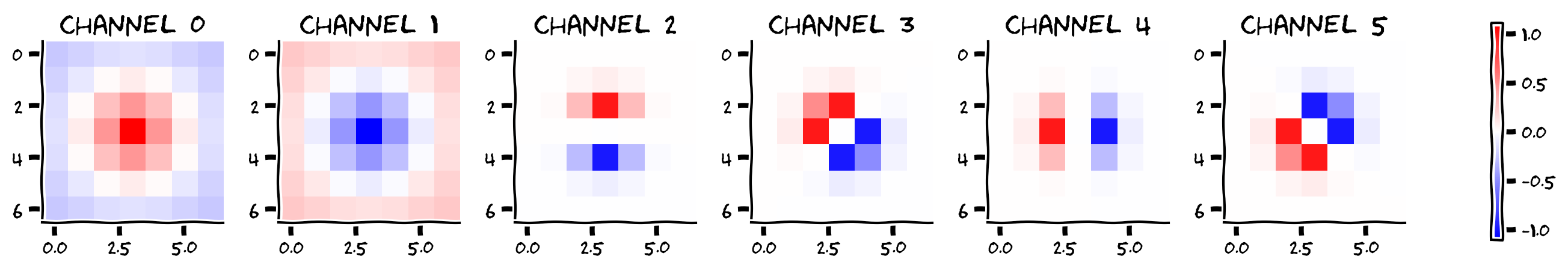
plot_weights(weights, channels=np.arange(0, out_channels))

解答を見る$

出力例:

# @title Submit your feedback
content_review(f"{feedback_prefix}_Visualizing_convolutional_filter_weights_Bonus_Exercise")

filters関数では、様々な向きの中心周辺フィルターとガボールフィルターを事前に作成しています。ガボールフィルター$は正の領域と負の領域が隣接し、フィルターのこれらの領域の向きが応答するエッジの向きを決定します。

視覚野では、HubelとWieselが単純細胞を発見しました。これは上記チャネル2-5のユニットに対応し、ガボールフィルターのようなものです。また、中心周辺フィルターに似た活動を示すニューロンもあり、これは上記の最初の2つの畳み込みチャネルに対応します。

さらにHubelとWieselは複雑細胞を発見しました。これらはバーの正確な位置に関わらず向き付きグレーティングに応答します（ここで見ている応答はバーの位置に特異的です）。これらの細胞はある程度の平行移動不変性を持ちます。畳み込みニューラルネットワークはこれを模倣しようとしています。例えば、グレーティングは少し動いても水平向きのままであり、猫は画像内の位置が変わっても猫のままです。

ボーナス考えてみよう 2: 複雑細胞

• どのようにして複雑細胞を作り、平行移動不変な応答を得ることができるでしょうか？
• 複数の向きに応答する細胞をどのように作るでしょうか？

解答を見る$

# @title Submit your feedback
content_review(f"{feedback_prefix}_Complex_cell_Bonus_Discussion")