![]()

チュートリアル 4: 非線形次元削減
第1週, 4日目: 次元削減
Neuromatch Academyによる
コンテンツ作成者: アレックス・カイコ・ガジック、ジョン・マレー
コンテンツレビュアー: ルーズベ・ファルフーディ、マット・クラウス、スピロス・チャブリス、リチャード・ガオ、マイケル・ワスコム、シッダールト・スレシュ、ナタリー・シャウォロンコウ、エラ・バティ
制作編集者: スピロス・チャブリス
チュートリアルの目的
チュートリアルの推定所要時間: 35分
このノートブックでは、次元削減がデータの可視化や構造推定にどのように役立つかを探ります。そのために、PCAと非線形次元削減手法であるt-SNEを比較します。
概要:
- PCAを使ってMNISTを2次元で可視化する。
- t-SNEを使ってMNISTを2次元で可視化する。
# @title Tutorial slides
# @markdown These are the slides for the videos in all tutorials today
from IPython.display import IFrame
link_id = "kaq2x"
print(f"If you want to download the slides: https://osf.io/download/{link_id}/")
IFrame(src=f"https://mfr.ca-1.osf.io/render?url=https://osf.io/{link_id}/?direct%26mode=render%26action=download%26mode=render", width=854, height=480)
セットアップ
# @title Install and import feedback gadget


from vibecheck import DatatopsContentReviewContainer
def content_review(notebook_section: str):
    return DatatopsContentReviewContainer(
        "",  # No text prompt
        notebook_section,
        {
            "url": "https://pmyvdlilci.execute-api.us-east-1.amazonaws.com/klab",
            "name": "neuromatch_cn",
            "user_key": "y1x3mpx5",
        },
    ).render()


feedback_prefix = "W1D4_T4"
# Imports
import numpy as np
import matplotlib.pyplot as plt# @title Figure Settings
import logging
logging.getLogger('matplotlib.font_manager').disabled = True
import ipywidgets as widgets # interactive display
%config InlineBackend.figure_format = 'retina'
plt.style.use("https://raw.githubusercontent.com/NeuromatchAcademy/course-content/main/nma.mplstyle")# @title Plotting Functions
def visualize_components(component1, component2, labels, show=True):
"""
Plots a 2D representation of the data for visualization with categories
labelled as different colors.
Args:
component1 (numpy array of floats) : Vector of component 1 scores
component2 (numpy array of floats) : Vector of component 2 scores
labels (numpy array of floats) : Vector corresponding to categories of
samples
Returns:
Nothing.
"""
plt.figure()
plt.scatter(x=component1, y=component2, c=labels, cmap='tab10')
plt.xlabel('Component 1')
plt.ylabel('Component 2')
plt.colorbar(ticks=range(10))
plt.clim(-0.5, 9.5)
if show:
plt.show()セクション0: 応用の紹介
# @title Video 1: PCA Applications
from ipywidgets import widgets
from IPython.display import YouTubeVideo
from IPython.display import IFrame
from IPython.display import display


class PlayVideo(IFrame):
  def __init__(self, id, source, page=1, width=400, height=300, **kwargs):
    self.id = id
    if source == 'Bilibili':
      src = f'https://player.bilibili.com/player.html?bvid={id}&page={page}'
    elif source == 'Osf':
      src = f'https://mfr.ca-1.osf.io/render?url=https://osf.io/download/{id}/?direct%26mode=render'
    super(PlayVideo, self).__init__(src, width, height, **kwargs)


def display_videos(video_ids, W=400, H=300, fs=1):
  tab_contents = []
  for i, video_id in enumerate(video_ids):
    out = widgets.Output()
    with out:
      if video_ids[i][0] == 'Youtube':
        video = YouTubeVideo(id=video_ids[i][1], width=W,
                             height=H, fs=fs, rel=0)
        print(f'Video available at https://youtube.com/watch?v={video.id}')
      else:
        video = PlayVideo(id=video_ids[i][1], source=video_ids[i][0], width=W,
                          height=H, fs=fs, autoplay=False)
        if video_ids[i][0] == 'Bilibili':
          print(f'Video available at https://www.bilibili.com/video/{video.id}')
        elif video_ids[i][0] == 'Osf':
          print(f'Video available at https://osf.io/{video.id}')
      display(video)
    tab_contents.append(out)
  return tab_contents


video_ids = [('Youtube', '2Zb93aOWioM'), ('Bilibili', 'BV1Jf4y1R7UZ')]
tab_contents = display_videos(video_ids, W=854, H=480)
tabs = widgets.Tab()
tabs.children = tab_contents
for i in range(len(tab_contents)):
  tabs.set_title(i, video_ids[i][0])
display(tabs)
# @title Submit your feedback
content_review(f"{feedback_prefix}_PCA_Applications_Video")セクション1: PCAを使ってMNISTを2次元で可視化する
この演習では、MNISTデータセットの最初のいくつかの成分を可視化して、データの構造の証拠を探します。ただし、このチュートリアルでは各画像のラベル(つまり0から9までのどの数字か)にも注目します。まず、以下のセルを実行してMNISTデータセットを再読み込みしてください(数秒かかります)。
from sklearn.datasets import fetch_openml

# Get images
mnist = fetch_openml(name='mnist_784', as_frame=False, parser='auto')
X_all = mnist.data

# Get labels
labels_all = np.array([int(k) for k in mnist.target])
注意: 完全なデータセットはとして、ラベルはlabels_allとして保存しています。
PCAを実行するために、ここではsklearnで実装されたメソッドを使用します。以下のセルを実行してPCAのパラメータを設定します。2次元で可視化するため、上位2成分のみを見ます。
from sklearn.decomposition import PCA

# Initializes PCA
pca_model = PCA(n_components=2)

# Performs PCA
pca_model.fit(X_all)
コーディング演習1: PCAを使ったMNISTの2次元可視化
以下のコードを完成させてPCAを実行し、上位2つの成分を可視化してください。より良い可視化のために、データの最初の2,000サンプルのみを使いましょう(このステップはt-SNEを次のセクションで高速化するためにも重要です。必ず行ってください!)
提案:
- データ行列を2,000サンプルに切り詰めます。ラベルの配列も同様に切り詰める必要があります。
- 切り詰めたデータにPCAを実行します。
visualize_components関数を使ってラベル付きデータをプロットします。
help(visualize_components)
help(pca_model.transform)
#################################################
## TODO for students: take only 2,000 samples and perform PCA
# Comment once you've completed the code
raise NotImplementedError("Student exercise: perform PCA")
#################################################
# Take only the first 2000 samples with the corresponding labels
X, labels = ...
# Perform PCA
scores = pca_model.transform(X)
# Plot the data and reconstruction
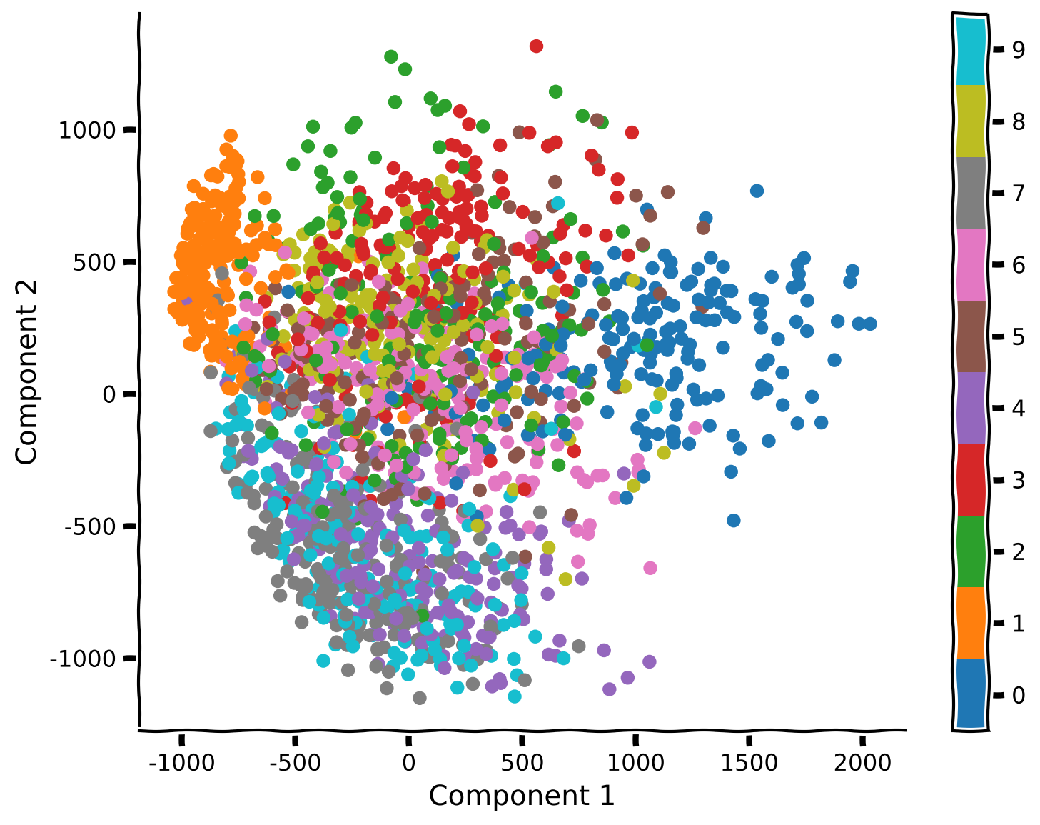
visualize_components(...)出力例:
# @title Submit your feedback
content_review(f"{feedback_prefix}_Visualization_of_MNIST_in_2D_using_PCA_Exercise")
考えてみよう 1: PCAによる可視化
- 何が見えますか?同じ数字に対応する異なるサンプルは一緒にクラスタリングされていますか?重なりは多いですか?
- いくつかの数字のペアは他よりも区別しやすく見えますか?
# @title Submit your feedback
content_review(f"{feedback_prefix}_PCA_Visualization_Discussion")
セクション 2: t-SNEを使ってMNISTを2Dで可視化する
チュートリアル開始からここまでの推定所要時間: 15分
# @title Video 2: Nonlinear Methods
from ipywidgets import widgets
from IPython.display import YouTubeVideo
from IPython.display import IFrame
from IPython.display import display


class PlayVideo(IFrame):
  def __init__(self, id, source, page=1, width=400, height=300, **kwargs):
    self.id = id
    if source == 'Bilibili':
      src = f'https://player.bilibili.com/player.html?bvid={id}&page={page}'
    elif source == 'Osf':
      src = f'https://mfr.ca-1.osf.io/render?url=https://osf.io/download/{id}/?direct%26mode=render'
    super(PlayVideo, self).__init__(src, width, height, **kwargs)


def display_videos(video_ids, W=400, H=300, fs=1):
  tab_contents = []
  for i, video_id in enumerate(video_ids):
    out = widgets.Output()
    with out:
      if video_ids[i][0] == 'Youtube':
        video = YouTubeVideo(id=video_ids[i][1], width=W,
                             height=H, fs=fs, rel=0)
        print(f'Video available at https://youtube.com/watch?v={video.id}')
      else:
        video = PlayVideo(id=video_ids[i][1], source=video_ids[i][0], width=W,
                          height=H, fs=fs, autoplay=False)
        if video_ids[i][0] == 'Bilibili':
          print(f'Video available at https://www.bilibili.com/video/{video.id}')
        elif video_ids[i][0] == 'Osf':
          print(f'Video available at https://osf.io/{video.id}')
      display(video)
    tab_contents.append(out)
  return tab_contents


video_ids = [('Youtube', '5Xpb0YaN5Ms'), ('Bilibili', 'BV14Z4y1u7HG')]
tab_contents = display_videos(video_ids, W=854, H=480)
tabs = widgets.Tab()
tabs.children = tab_contents
for i in range(len(tab_contents)):
  tabs.set_title(i, video_ids[i][0])
display(tabs)
# @title Submit your feedback
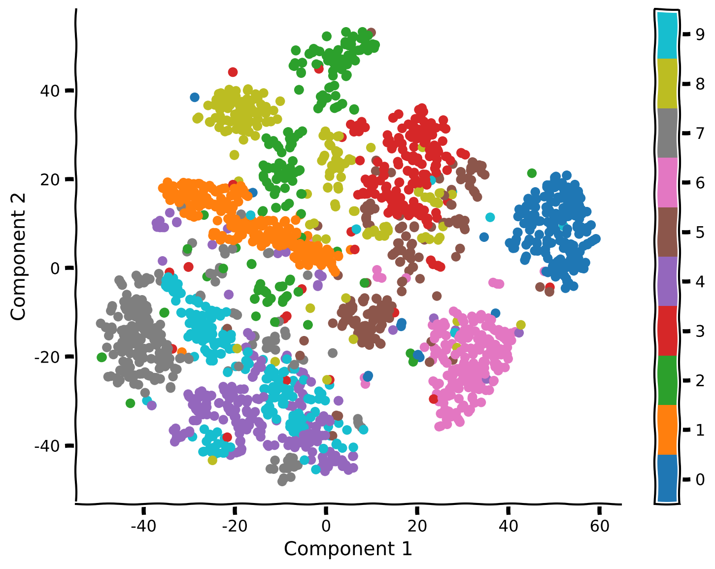
content_review(f"{feedback_prefix}_Nonlinear_methods_Video")次に、非線形次元削減手法であるt-SNEを使って同じデータを解析します。t-SNEは高次元データを2Dまたは3Dで可視化するのに便利です。以下のセルを実行して始めましょう。
from sklearn.manifold import TSNE
tsne_model = TSNE(n_components=2, perplexity=30, random_state=2020)
コーディング演習 2.1: MNISTにt-SNEを適用する
まず、t-SNEをデータに適用して、より多くの構造が見えるか探ります。上のセルでは、埋め込み(すなわちデータの低次元表現)を見つけるために使うパラメータを定義し、それらをmodelに保存しました。t-SNEをデータに適用するには、model.fit_transform関数を使います。
ヒント:
model.fit_transform関数を使ってt-SNEを実行しましょう。- 結果のデータを
visualize_componentsでプロットしましょう。
help(tsne_model.fit_transform)#################################################
## TODO for students
# Comment once you've completed the code
raise NotImplementedError("Student exercise: perform t-SNE")
#################################################
# Perform t-SNE
embed = ...
# Visualize the data
visualize_components(..., ..., labels)例の出力:
# @title Submit your feedback
content_review(f"{feedback_prefix}_Apply_tSNE_on_MNIST_Exercise")
コーディング演習 2.2: 異なるパープレキシティでt-SNEを実行する
PCAとは異なり、t-SNEにはパープレキシティという自由パラメータがあり、これは大まかにグローバル情報とローカル情報の重み付けを決めます。ここでは、パープレキシティが結果の解釈にどのように影響するかを見てみましょう。
手順:
- パープレキシティを50、5、2にしてt-SNEを再実行します(上記のように
TSNE関数で再初期化するのを忘れずに)。
def explore_perplexity(values, X, labels):
"""
Plots a 2D representation of the data for visualization with categories
labeled as different colors using different perplexities.
Args:
values (list of floats) : list with perplexities to be visualized
X (np.ndarray of floats) : matrix with the dataset
labels (np.ndarray of int) : array with the labels
Returns:
Nothing.
"""
for perp in values:
#################################################
## TO DO for students: Insert your code here to redefine the t-SNE "model"
## while setting the perplexity perform t-SNE on the data and plot the
## results for perplexity = 50, 5, and 2 (set random_state to 2020
# Comment these lines when you complete the function
raise NotImplementedError("Student Exercise! Explore t-SNE with different perplexity")
#################################################
# Perform t-SNE
tsne_model = ...
embed = tsne_model.fit_transform(X)
visualize_components(embed[:, 0], embed[:, 1], labels, show=False)
plt.title(f"perplexity: {perp}")
# Visualize
values = [50, 5, 2]
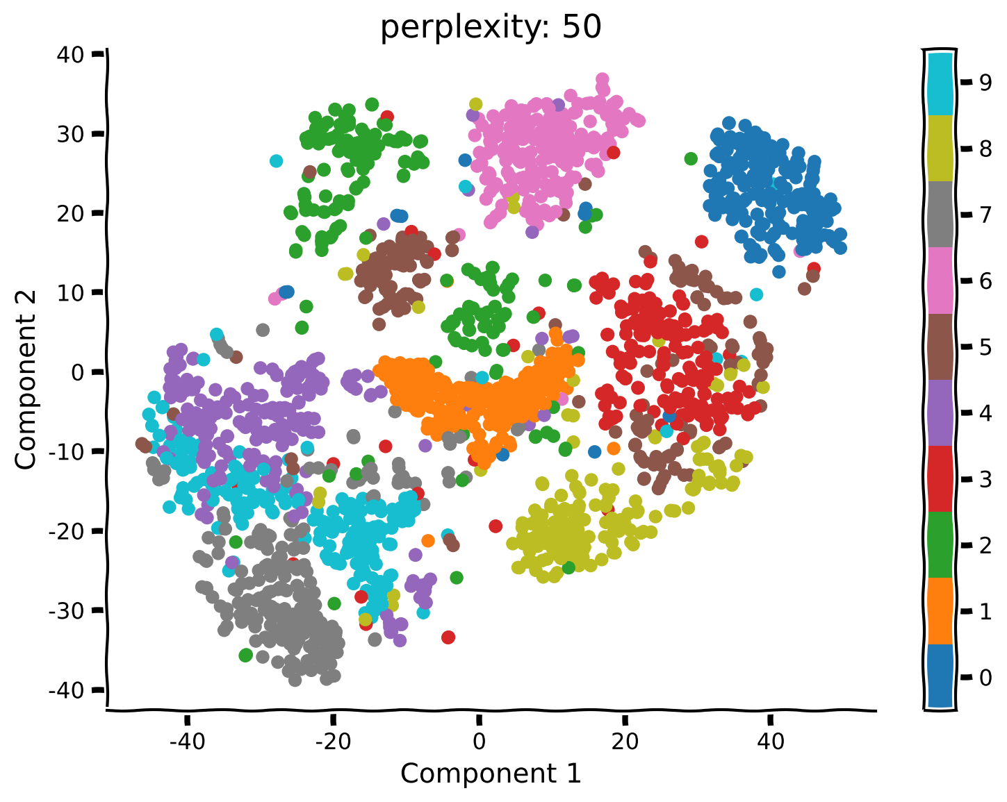
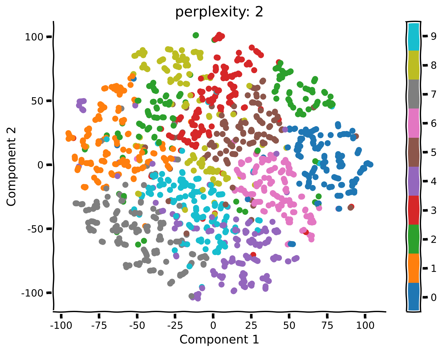
explore_perplexity(values, X, labels)例の出力:

# @title Submit your feedback
content_review(f"{feedback_prefix}_Run_tSNE_with_different_perplexities_Exercise")
考えてみよう 2: t-SNEの可視化
- パープレキシティ50の前回の結果と比べて何が変わりましたか?以前とは異なる構造のクラスターは見えますか?
- パープレキシティが5または2の場合、埋め込みの構造はどのように変わりましたか?
# @title Submit your feedback
content_review(f"{feedback_prefix}_tSNE_Visualization_Discussion")
まとめ
チュートリアルの推定所要時間: 35分
- 線形次元削減と非線形次元削減の違いを学びました。非線形手法はより強力な場合がありますが、ノイズに敏感になることもあります。一方、線形手法はシンプルで頑健なため有用です。
- データ可視化においてPCAとt-SNEを比較しました。t-SNEを使うことで、異なる数字に対応するクラスターを可視化できました。PCAは一部のクラスター(例:0と1)を分離できましたが、全体的には性能が劣りました。
- ただし、t-SNEの結果はパープレキシティの選択によって変わることがあります。詳細を知りたい方は、Wattenbergら, 2016年のDistill論文をおすすめします。