チュートリアル 3: 次元削減と再構成

第1週第4日目: 次元削減

Neuromatch Academyによる

コンテンツ作成者: アレックス・カイコ・ガジック、ジョン・マレー

コンテンツレビュアー: ルーズベ・ファルフーディ、マット・クラウス、スピロス・チャブリス、リチャード・ガオ、マイケル・ワスコム、シッダールト・スレシュ、ナタリー・シャウォロンコウ、エラ・バティ

制作編集者: スピロス・チャブリス

チュートリアルの目標

チュートリアルの推定所要時間: 50分

このノートブックでは、機械学習アルゴリズムのベンチマークによく使われる古典的なデータセットMNISTを用いて、PCAによる次元削減の適用方法を学びます。また、PCAを使った再構成とノイズ除去の方法も学びます。

概要:

MNISTに対してPCAを実行する
分散説明率を計算する
異なる数の主成分でデータを再構成する
（ボーナス）PCAを用いたノイズ除去を調べる

MNISTデータセットについて詳しくはこちら$をご覧ください。

# @title Tutorial slides
# @markdown These are the slides for the videos in all tutorials today
from IPython.display import IFrame
link_id = "kaq2x"
print(f"If you want to download the slides: https://osf.io/download/{link_id}/")
IFrame(src=f"https://mfr.ca-1.osf.io/render?url=https://osf.io/{link_id}/?direct%26mode=render%26action=download%26mode=render", width=854, height=480)

セットアップ

# @title Install and import feedback gadget


from vibecheck import DatatopsContentReviewContainer
def content_review(notebook_section: str):
    return DatatopsContentReviewContainer(
        "",  # No text prompt
        notebook_section,
        {
            "url": "https://pmyvdlilci.execute-api.us-east-1.amazonaws.com/klab",
            "name": "neuromatch_cn",
            "user_key": "y1x3mpx5",
        },
    ).render()


feedback_prefix = "W1D4_T3"

# Imports
import numpy as np
import matplotlib.pyplot as plt

# @title Figure Settings
import logging
logging.getLogger('matplotlib.font_manager').disabled = True

import ipywidgets as widgets  # interactive display
%config InlineBackend.figure_format = 'retina'
plt.style.use("https://raw.githubusercontent.com/NeuromatchAcademy/course-content/main/nma.mplstyle")

# @title Plotting Functions

def plot_variance_explained(variance_explained):
  """
  Plots eigenvalues.

  Args:
    variance_explained (numpy array of floats) : Vector of variance explained
                                                 for each PC

  Returns:
    Nothing.

  """

  plt.figure()
  plt.plot(np.arange(1, len(variance_explained) + 1), variance_explained,
           '--k')
  plt.xlabel('Number of components')
  plt.ylabel('Variance explained')
  plt.show()


def plot_MNIST_reconstruction(X, X_reconstructed, keep_dims):
  """
  Plots 9 images in the MNIST dataset side-by-side with the reconstructed
  images.

  Args:
    X (numpy array of floats)               : Data matrix each column
                                              corresponds to a different
                                              random variable
    X_reconstructed (numpy array of floats) : Data matrix each column
                                              corresponds to a different
                                              random variable
    keep_dims (int)                         : Dimensions to keep

  Returns:
    Nothing.
  """

  plt.figure()
  ax = plt.subplot(121)
  k = 0
  for k1 in range(3):
    for k2 in range(3):
      k = k + 1
      plt.imshow(np.reshape(X[k, :], (28, 28)),
                 extent=[(k1 + 1) * 28, k1 * 28, (k2 + 1) * 28, k2 * 28],
                 vmin=0, vmax=255)
  plt.xlim((3 * 28, 0))
  plt.ylim((3 * 28, 0))
  plt.tick_params(axis='both', which='both', bottom=False, top=False,
                  labelbottom=False)
  ax.set_xticks([])
  ax.set_yticks([])
  plt.title('Data')
  plt.clim([0, 250])
  ax = plt.subplot(122)
  k = 0
  for k1 in range(3):
    for k2 in range(3):
      k = k + 1
      plt.imshow(np.reshape(np.real(X_reconstructed[k, :]), (28, 28)),
                 extent=[(k1 + 1) * 28, k1 * 28, (k2 + 1) * 28, k2 * 28],
                 vmin=0, vmax=255)
  plt.xlim((3 * 28, 0))
  plt.ylim((3 * 28, 0))
  plt.tick_params(axis='both', which='both', bottom=False, top=False,
                  labelbottom=False)
  ax.set_xticks([])
  ax.set_yticks([])
  plt.clim([0, 250])
  plt.title(f'Reconstructed K: {keep_dims}')
  plt.tight_layout()
  plt.show()


def plot_MNIST_sample(X):
  """
  Plots 9 images in the MNIST dataset.

  Args:
     X (numpy array of floats) : Data matrix each column corresponds to a
                                 different random variable

  Returns:
    Nothing.

  """

  fig, ax = plt.subplots()
  k = 0
  for k1 in range(3):
    for k2 in range(3):
      k = k + 1
      plt.imshow(np.reshape(X[k, :], (28, 28)),
                 extent=[(k1 + 1) * 28, k1 * 28, (k2+1) * 28, k2 * 28],
                 vmin=0, vmax=255)
  plt.xlim((3 * 28, 0))
  plt.ylim((3 * 28, 0))
  plt.tick_params(axis='both', which='both', bottom=False, top=False,
                  labelbottom=False)
  plt.clim([0, 250])
  ax.set_xticks([])
  ax.set_yticks([])
  plt.show()


def plot_MNIST_weights(weights):
  """
  Visualize PCA basis vector weights for MNIST. Red = positive weights,
  blue = negative weights, white = zero weight.

  Args:
     weights (numpy array of floats) : PCA basis vector

  Returns:
     Nothing.
  """

  fig, ax = plt.subplots()
  plt.imshow(np.real(np.reshape(weights, (28, 28))), cmap='seismic')
  plt.tick_params(axis='both', which='both', bottom=False, top=False,
                  labelbottom=False)
  plt.clim(-.15, .15)
  plt.colorbar(ticks=[-.15, -.1, -.05, 0, .05, .1, .15])
  ax.set_xticks([])
  ax.set_yticks([])
  plt.show()


def plot_eigenvalues(evals, xlimit=False):
  """
  Plots eigenvalues.

  Args:
     (numpy array of floats) : Vector of eigenvalues
     (boolean) : enable plt.show()
  Returns:
    Nothing.

  """

  plt.figure()
  plt.plot(np.arange(1, len(evals) + 1), evals, 'o-k')
  plt.xlabel('Component')
  plt.ylabel('Eigenvalue')
  plt.title('Scree plot')
  if xlimit:
    plt.xlim([0, 100])  # limit x-axis up to 100 for zooming
  plt.show()

# @title Helper Functions

def add_noise(X, frac_noisy_pixels):
  """
  Randomly corrupts a fraction of the pixels by setting them to random values.

  Args:
     X (numpy array of floats)  : Data matrix
     frac_noisy_pixels (scalar) : Fraction of noisy pixels

  Returns:
     (numpy array of floats)    : Data matrix + noise

  """

  X_noisy = np.reshape(X, (X.shape[0] * X.shape[1]))
  N_noise_ixs = int(X_noisy.shape[0] * frac_noisy_pixels)
  noise_ixs = np.random.choice(X_noisy.shape[0], size=N_noise_ixs,
                               replace=False)
  X_noisy[noise_ixs] = np.random.uniform(0, 255, noise_ixs.shape)
  X_noisy = np.reshape(X_noisy, (X.shape[0], X.shape[1]))

  return X_noisy


def change_of_basis(X, W):
  """
  Projects data onto a new basis.

  Args:
    X (numpy array of floats) : Data matrix each column corresponding to a
                                different random variable
    W (numpy array of floats) : new orthonormal basis columns correspond to
                                basis vectors

  Returns:
    (numpy array of floats)   : Data matrix expressed in new basis
  """

  Y = np.matmul(X, W)

  return Y


def get_sample_cov_matrix(X):
  """
  Returns the sample covariance matrix of data X.

  Args:
    X (numpy array of floats) : Data matrix each column corresponds to a
                                different random variable

  Returns:
    (numpy array of floats)   : Covariance matrix
"""

  X = X - np.mean(X, 0)
  cov_matrix = 1 / X.shape[0] * np.matmul(X.T, X)
  return cov_matrix


def sort_evals_descending(evals, evectors):
  """
  Sorts eigenvalues and eigenvectors in decreasing order. Also aligns first two
  eigenvectors to be in first two quadrants (if 2D).

  Args:
    evals (numpy array of floats)    :   Vector of eigenvalues
    evectors (numpy array of floats) :   Corresponding matrix of eigenvectors
                                         each column corresponds to a different
                                         eigenvalue

  Returns:
    (numpy array of floats)          : Vector of eigenvalues after sorting
    (numpy array of floats)          : Matrix of eigenvectors after sorting
  """

  index = np.flip(np.argsort(evals))
  evals = evals[index]
  evectors = evectors[:, index]
  if evals.shape[0] == 2:
    if np.arccos(np.matmul(evectors[:, 0],
                           1 / np.sqrt(2) * np.array([1, 1]))) > np.pi / 2:
      evectors[:, 0] = -evectors[:, 0]
    if np.arccos(np.matmul(evectors[:, 1],
                           1 / np.sqrt(2)*np.array([-1, 1]))) > np.pi / 2:
      evectors[:, 1] = -evectors[:, 1]

  return evals, evectors


def pca(X):
  """
  Performs PCA on multivariate data. Eigenvalues are sorted in decreasing order

  Args:
     X (numpy array of floats) :   Data matrix each column corresponds to a
                                   different random variable

  Returns:
    (numpy array of floats)    : Data projected onto the new basis
    (numpy array of floats)    : Corresponding matrix of eigenvectors
    (numpy array of floats)    : Vector of eigenvalues

  """

  X = X - np.mean(X, 0)
  cov_matrix = get_sample_cov_matrix(X)
  evals, evectors = np.linalg.eigh(cov_matrix)
  evals, evectors = sort_evals_descending(evals, evectors)
  score = change_of_basis(X, evectors)

  return score, evectors, evals

セクション0: PCAのイントロダクション

# @title Video 1: PCA for dimensionality reduction
from ipywidgets import widgets
from IPython.display import YouTubeVideo
from IPython.display import IFrame
from IPython.display import display


class PlayVideo(IFrame):
  def __init__(self, id, source, page=1, width=400, height=300, **kwargs):
    self.id = id
    if source == 'Bilibili':
      src = f'https://player.bilibili.com/player.html?bvid={id}&page={page}'
    elif source == 'Osf':
      src = f'https://mfr.ca-1.osf.io/render?url=https://osf.io/download/{id}/?direct%26mode=render'
    super(PlayVideo, self).__init__(src, width, height, **kwargs)


def display_videos(video_ids, W=400, H=300, fs=1):
  tab_contents = []
  for i, video_id in enumerate(video_ids):
    out = widgets.Output()
    with out:
      if video_ids[i][0] == 'Youtube':
        video = YouTubeVideo(id=video_ids[i][1], width=W,
                             height=H, fs=fs, rel=0)
        print(f'Video available at https://youtube.com/watch?v={video.id}')
      else:
        video = PlayVideo(id=video_ids[i][1], source=video_ids[i][0], width=W,
                          height=H, fs=fs, autoplay=False)
        if video_ids[i][0] == 'Bilibili':
          print(f'Video available at https://www.bilibili.com/video/{video.id}')
        elif video_ids[i][0] == 'Osf':
          print(f'Video available at https://osf.io/{video.id}')
      display(video)
    tab_contents.append(out)
  return tab_contents


video_ids = [('Youtube', 'oO0bbInoO_0'), ('Bilibili', 'BV1up4y1S7xs')]
tab_contents = display_videos(video_ids, W=854, H=480)
tabs = widgets.Tab()
tabs.children = tab_contents
for i in range(len(tab_contents)):
  tabs.set_title(i, video_ids[i][0])
display(tabs)

# @title Submit your feedback
content_review(f"{feedback_prefix}_PCA_for_dimensionality_reduction_Video")

セクション1: MNISTに対してPCAを実行する

MNISTデータセットは、7万枚の手書き数字の画像で構成されています。各画像は28×28ピクセルのグレースケール画像です。便宜上、各28×28ピクセルの画像は1次元に展開され、784（=28×28）要素のベクトルとして表されます。したがって、データセット全体は7万行×784列の行列として表されます。各行は異なる画像を、各列は異なるピクセルを表します。

以下のセルを実行してMNISTデータセットを読み込み、最初の9枚の画像をプロットしてください。読み込みには数分かかる場合があります。

from sklearn.datasets import fetch_openml

# GET mnist data
mnist = fetch_openml(name='mnist_784', as_frame=False, parser='auto')
X = mnist.data

# Visualize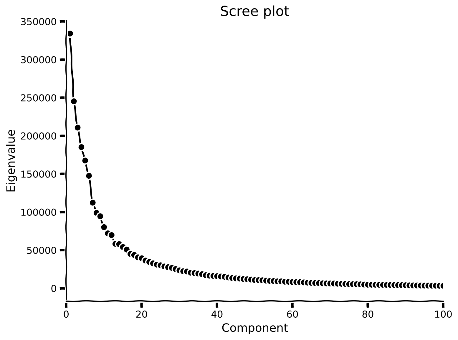
plot_MNIST_sample(X)

MNISTデータセットの外在的次元数は784で、前のチュートリアルで使った2次元の例よりはるかに高いです！このデータを理解するために、次元削減を使います。しかしまず、データの内在的次元数 $K$ を決定する必要があります。その一つの方法は、スクリープロットで「ひじ」の位置を探し、どの固有値が重要かを判断することです。

コーディング演習1: MNISTのスクリープロット

この演習では、MNISTデータセットのスクリープロットを調べます。

手順:

チュートリアル2で使った関数pcaを用いてデータセットにPCAを実行し、スクリープロットを確認します。
固有値が（目視で）ゼロに近づくのはいつ頃かを確認してください。（ヒント: plt.xlimを使ってプロットの一部を拡大できます）

help(pca)

#################################################
## TODO for students
# Fill out function and remove
raise NotImplementedError("Student exercise: perform PCA and visualize scree plot")
#################################################

# Perform PCA
score, evectors, evals = ...

# Plot the eigenvalues
plot_eigenvalues(evals, xlimit=True)  # limit x-axis up to 100 for zooming

解答を見る$

出力例:

# @title Submit your feedback
content_review(f"{feedback_prefix}_Scree_plot_of_MNIST_Exercise")

セクション2: 分散説明率の計算

チュートリアル開始からここまでの推定所要時間: 15分

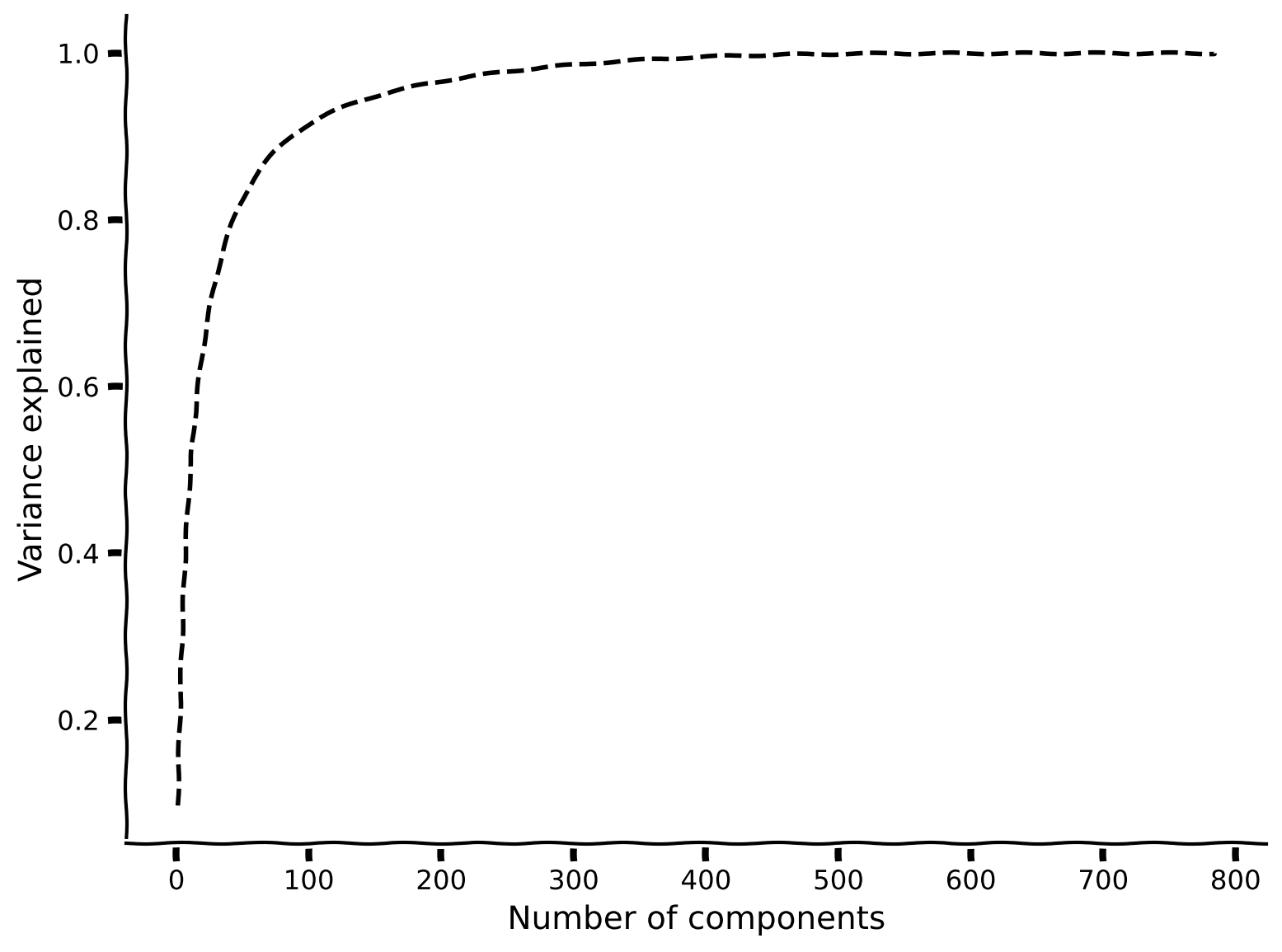
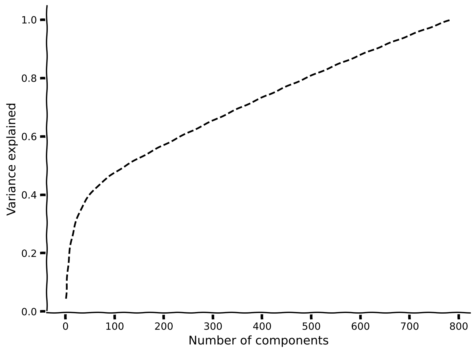
スクリープロットを見ると、ほとんどの固有値はゼロに近く、100未満の固有値だけが大きな値を持っています。内在的次元数を決めるもう一つの一般的な方法は、分散説明率を考慮することです。これは、上位 $K$ 成分によって説明される全分散の割合の累積プロットで調べられます。すなわち、

\text{分散説明率} = \frac{\sum_{i=1}^K \lambda_i}{\sum_{i=1}^N \lambda_i}

ここで $\lambda_i$ は $i$ 番目の固有値、 $N$ は成分の総数（元のデータの次元数）です。

内在的次元数は、データの全分散の大部分（例えば90%）を説明するのに必要な $K$ で定量化されることが多いです。

コーディング演習2: 分散説明率のプロット

この演習では、分散説明率をプロットします。

手順:

以下の関数を完成させて、主成分数に対する分散説明率の割合を計算してください。ヒント: np.cumsumを使います。
plot_variance_explainedを使って分散説明率をプロットしてください。

質問:

90%の分散を説明するのに必要な主成分数はいくつですか？
このデータセットの内在的次元数は外在的次元数と比べてどうですか？

def get_variance_explained(evals):
  """
  Calculates variance explained from the eigenvalues.

  Args:
    evals (numpy array of floats) : Vector of eigenvalues

  Returns:
    (numpy array of floats)       : Vector of variance explained

  """

  #################################################
  ## TO DO for students: calculate the explained variance using the equation
  ## from Section 2.
  # Comment once you've filled in the function
  raise NotImplementedError("Student exercise: calculate explain variance!")
  #################################################

  # Cumulatively sum the eigenvalues
  csum = ...

  # Normalize by the sum of eigenvalues
  variance_explained = ...

  return variance_explained


# Calculate the variance explained
variance_explained = get_variance_explained(evals)

# Visualize
plot_variance_explained(variance_explained)

解答を見る$

出力例:

# @title Submit your feedback
content_review(f"{feedback_prefix}_Plot_the_explained_variance_Exercise")

セクション3: 異なる数の主成分でデータを再構成する

チュートリアル開始からここまでの推定所要時間: 25分

# @title Video 2: Data Reconstruction
from ipywidgets import widgets
from IPython.display import YouTubeVideo
from IPython.display import IFrame
from IPython.display import display


class PlayVideo(IFrame):
  def __init__(self, id, source, page=1, width=400, height=300, **kwargs):
    self.id = id
    if source == 'Bilibili':
      src = f'https://player.bilibili.com/player.html?bvid={id}&page={page}'
    elif source == 'Osf':
      src = f'https://mfr.ca-1.osf.io/render?url=https://osf.io/download/{id}/?direct%26mode=render'
    super(PlayVideo, self).__init__(src, width, height, **kwargs)


def display_videos(video_ids, W=400, H=300, fs=1):
  tab_contents = []
  for i, video_id in enumerate(video_ids):
    out = widgets.Output()
    with out:
      if video_ids[i][0] == 'Youtube':
        video = YouTubeVideo(id=video_ids[i][1], width=W,
                             height=H, fs=fs, rel=0)
        print(f'Video available at https://youtube.com/watch?v={video.id}')
      else:
        video = PlayVideo(id=video_ids[i][1], source=video_ids[i][0], width=W,
                          height=H, fs=fs, autoplay=False)
        if video_ids[i][0] == 'Bilibili':
          print(f'Video available at https://www.bilibili.com/video/{video.id}')
        elif video_ids[i][0] == 'Osf':
          print(f'Video available at https://osf.io/{video.id}')
      display(video)
    tab_contents.append(out)
  return tab_contents


video_ids = [('Youtube', 'ZCUhW26AdBQ'), ('Bilibili', 'BV1XK4y1s7KF')]
tab_contents = display_videos(video_ids, W=854, H=480)
tabs = widgets.Tab()
tabs.children = tab_contents
for i in range(len(tab_contents)):
  tabs.set_title(i, video_ids[i][0])
display(tabs)

# @title Submit your feedback
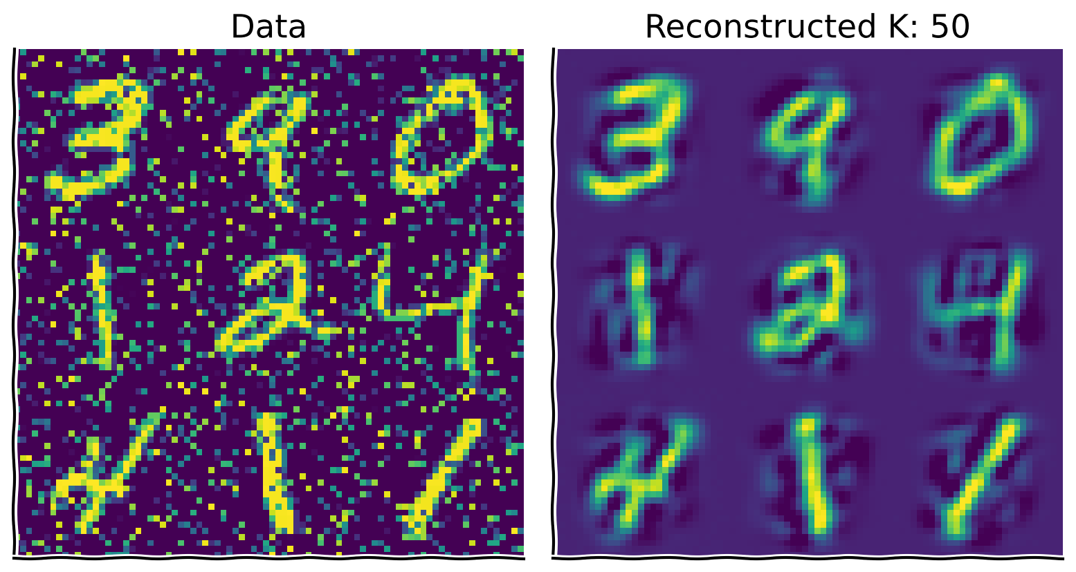
content_review(f"{feedback_prefix}_Data_reconstruction_Video")

ここまでで、データの上位約100個の主成分でほとんどの分散を説明できることがわかりました。この事実を利用して、次元削減を行います。つまり、784ピクセルすべてのサンプルを保存する代わりに、100個の成分だけを使ってデータを保存します。驚くべきことに、上位100個の成分だけでデータの構造の多くを再構成できます。これを理解するために、PCAを行う際にデータ $\bf X$ を共分散行列の固有ベクトルに射影したことを思い出してください：

\bf S = X W

$\bf W$ は直交行列なので、 ${\bf W}^{-1} = {\bf W}^\top$ です。したがって、両辺に ${\bf W}^\top$ を掛けると、

{\bf X = S W}^\top.

これにより、スコア行列 $\bf S$ と負荷行列 $\bf W$ からデータ行列を再構成する方法が得られます。低次元近似からデータを再構成するには、これらの行列を切り詰めればよいです。 $\bf S$ と $\bf W$ の最初の $K$ 列だけを持つ行列をそれぞれ ${\bf S}_{1:K}$ と ${\bf W}_{1:K}$ とすると、再構成は次のようになります：

{\bf \hat X = S}_{1:K} ({\bf W}_{1:K})^\top.

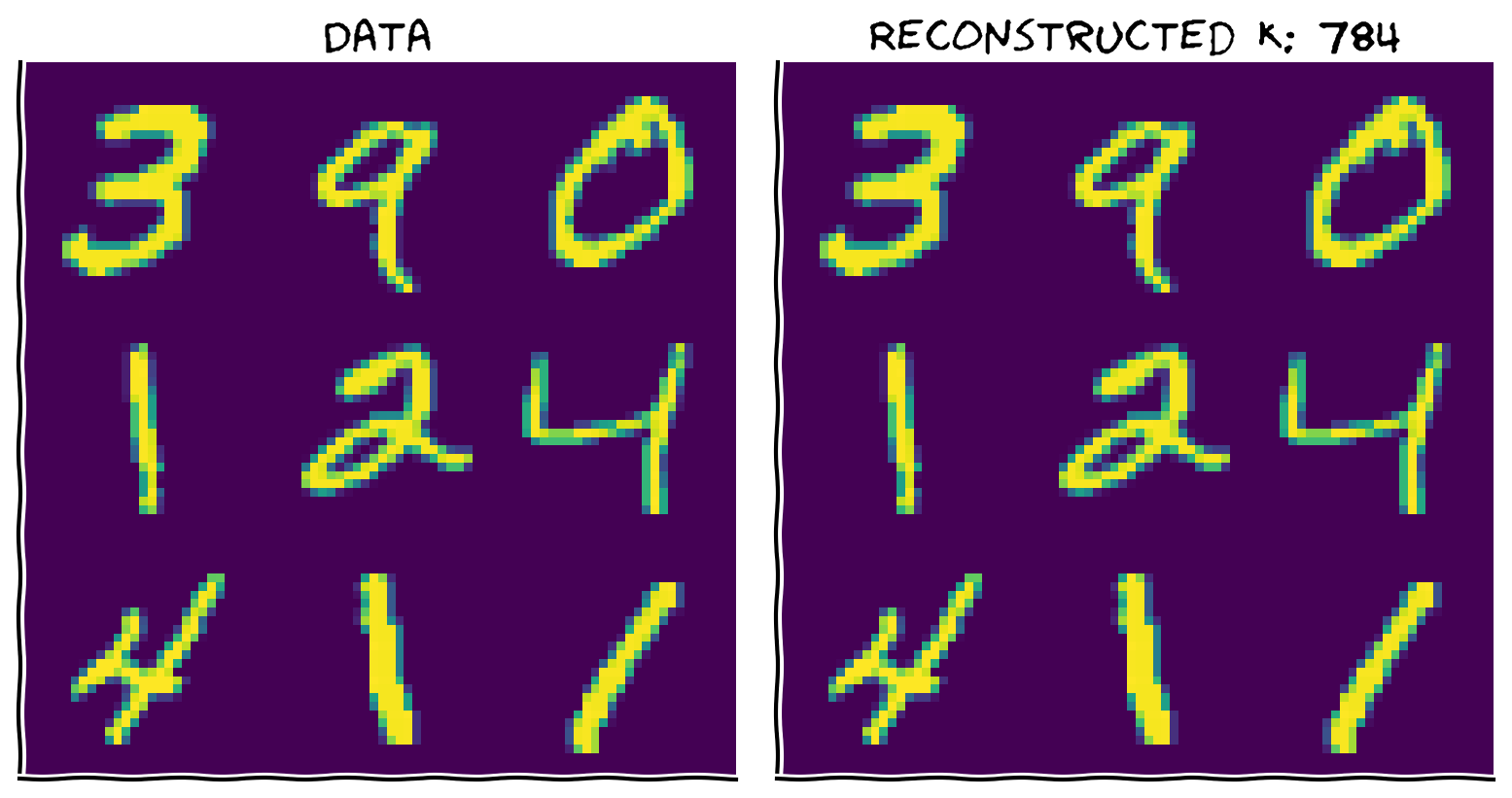
コーディング演習3: データの再構成

以下の関数を完成させて、異なる数の主成分を使ってデータを再構成してください。

手順:

重みとスコアに基づいてデータを再構成する関数を完成させてください。平均を加えるのを忘れないでください！
関数が正しく動作することを確認するために、すべての $K=784$ 成分を使ってデータを再構成してください。2つの画像は同一に見えるはずです。

def reconstruct_data(score, evectors, X_mean, K):
  """
  Reconstruct the data based on the top K components.

  Args:
    score (numpy array of floats)    : Score matrix
    evectors (numpy array of floats) : Matrix of eigenvectors
    X_mean (numpy array of floats)   : Vector corresponding to data mean
    K (scalar)                       : Number of components to include

  Returns:
    (numpy array of floats)          : Matrix of reconstructed data

  """

  #################################################
  ## TO DO for students: Reconstruct the original data in X_reconstructed
  # Comment once you've filled in the function
  raise NotImplementedError("Student exercise: reconstructing data function!")
  #################################################

  # Reconstruct the data from the score and eigenvectors
  # Don't forget to add the mean!!
  X_reconstructed =  ...

  return X_reconstructed


K = 784  # data dimensions

# Reconstruct the data based on all components
X_mean = np.mean(X, 0)
X_reconstructed = reconstruct_data(score, evectors, X_mean, K)

# Plot the data and reconstruction
plot_MNIST_reconstruction(X, X_reconstructed, K)

解答を見る$

出力例:

# @title Submit your feedback
content_review(f"{feedback_prefix}_Data_reconstruction_Exercise")

インタラクティブデモ 3: 異なる数の主成分を使ってデータ行列を再構成する

以下のコードを実行し、スライダーを操作して異なる数の主成分を使ってデータ行列を再構成してみましょう。

目視で数字を再構成するのに必要な主成分はいくつですか？これはデータの内在的次元性とどのように関係していますか？
単一の主成分だけでデータにどんな情報が見えますか？

# @markdown Make sure you execute this cell to enable the widget!

def refresh(K=100):
  X_reconstructed = reconstruct_data(score, evectors, X_mean, K)
  plot_MNIST_reconstruction(X, X_reconstructed, K)


_ = widgets.interact(refresh, K=(1, 784, 10))

解答を見る$

# @title Submit your feedback
content_review(f"{feedback_prefix}_Reconstruct_the_data_matrix_using_different_numbers_of_PCs_Interactive_Demo_and_discussion")

セクション4: PCA成分の可視化

チュートリアル開始からここまでの推定所要時間: 40分

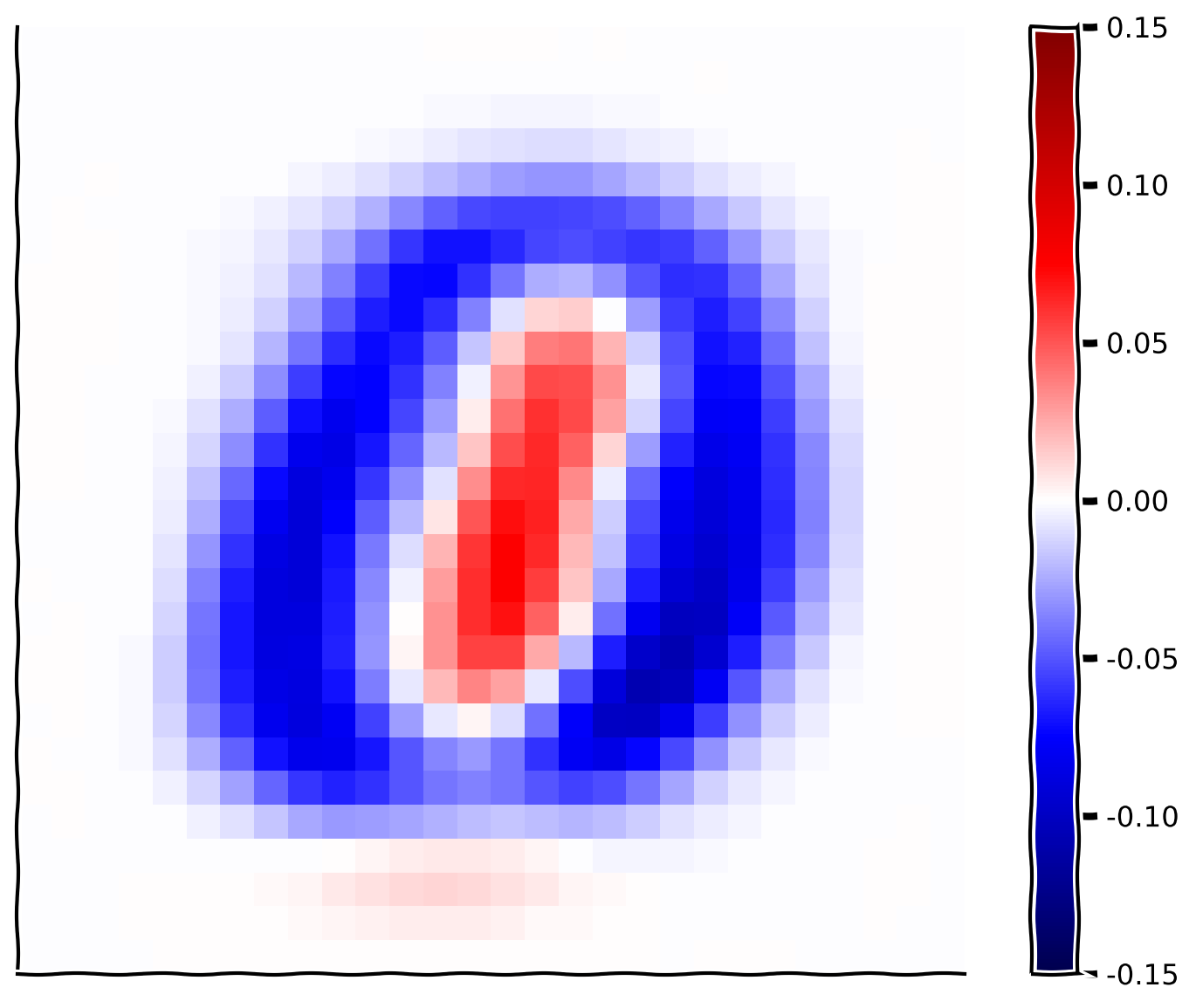
コーディング演習4: 重みの可視化

次に、最初の主成分に対応する重みを可視化して詳しく見てみましょう。

手順:

plot_MNIST_weights を入力して最初の基底ベクトルの重みを可視化します。
どんな構造が見えますか？どのピクセルが強い正の重みを持っていますか？どのピクセルが強い負の重みを持っていますか？この基底ベクトルはどんな種類の画像を区別しますか？（ヒント：1成分の最後のデモを思い出してください）
2番目と3番目の基底ベクトルも可視化してみましょう。何か構造が見えますか？100番目の基底ベクトルは？500番目は？700番目は？

help(plot_MNIST_weights)

################################################################
# Comment once you've filled in the function
raise NotImplementedError("Student exercise: visualize PCA components")
################################################################

# Plot the weights of the first principal component
plot_MNIST_weights(...)

解答を見る$

出力例:

# @title Submit your feedback
content_review(f"{feedback_prefix}_Visualization_of_the_weights_Exercise")

まとめ

チュートリアルの推定所要時間: 50分

このチュートリアルでは、主成分分析（PCA）を用いて上位の主成分を選択することで次元削減を行う方法を学びました。これは、神経データにおいて内在的次元数 ( $K$ ) が外在的次元数 ( $N$ ) よりも小さいことが多いため有用です。 $K$ は分散のある割合を捉えるのに必要な固有値の数を選ぶことで推定できます。
また、上位 $K$ 個の主成分を使って元のデータの近似を再構成する方法も学びました。実際、PCAの別の定式化は、再構成誤差を最小化する $K$ 次元空間を見つけることです。
ノイズは見かけ上の内在的次元数を膨らませる傾向がありますが、高次の成分は新しい構造ではなくノイズを反映しています。PCAはノイズの多い高次成分を除去することでデータのノイズ除去にも使えます。
MNISTでは、最初の主成分に対応する重みが0と1を区別しているように見えます。これについては次のチュートリアルでデータ可視化への影響を議論します。

記法

\begin{align}
K & $\quad \text{選択された主成分の数}$ \
N & $\quad \text{主成分の総数}$ \
$\bf W$ & $\quad \text{重み（ロード行列）}$ \
{ $\bf X}$ & $\quad \text{元のデータ行列}$ \
$\bf S$ & $\quad \text{射影後の行列（スコア）}$ \
{ $\bf S}_{1$ :K} & $\quad \text{スコア行列 } \bf S \text{ の最初の } K \text{ 列}$ \
{ $\bf W}_{1$ :K} & $\quad \text{重み行列 } \bf W \text{ の最初の } K \text{ 列}$ \
\end{align}

ボーナス

ボーナスセクション1: PCAを使ったノイズ除去の検証

この講義では、PCAが再構成誤差を最小化する最適な低次元基底を見つけることを学びました。この特性により、PCAはノイズの混入したデータのノイズ除去に有用です。

ボーナスコーディング演習1: データにノイズを加える

この演習では、元のデータに塩胡椒ノイズを加え、その影響を固有値で確認します。

手順:

関数 add_noise を使ってピクセルの20%にノイズを加えます。
その後、PCAを実行して分散説明率をプロットします。90%の分散を説明するのに必要な主成分はいくつですか？元のデータと比べてどうですか？

help(add_noise)

#################################################
## TO DO for students
# Comment once you've filled in the function
raise NotImplementedError("Student exercise: make MNIST noisy and compute PCA!")
#################################################

np.random.seed(2020)  # set random seed

# Add noise to data
X_noisy = ...

# Perform PCA on noisy data
score_noisy, evectors_noisy, evals_noisy = ...

# Compute variance explained
variance_explained_noisy = ...

# Visualize
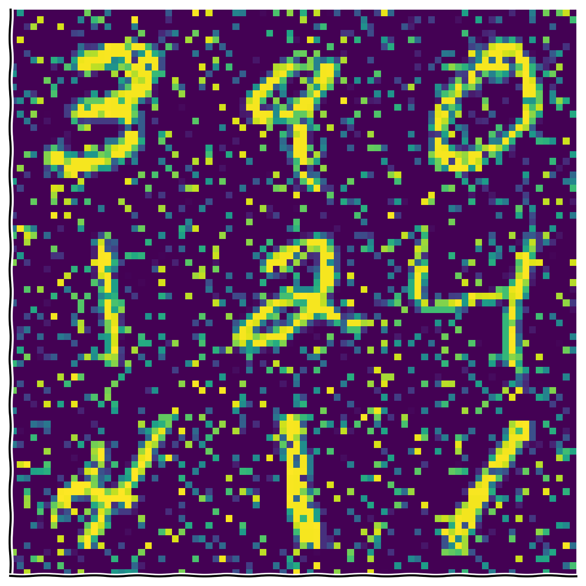
plot_MNIST_sample(X_noisy)
plot_variance_explained(variance_explained_noisy)

解答を見る$

出力例:

# @title Submit your feedback
content_review(f"{feedback_prefix}_Add_noise_to_the_data_Bonus_Exercise")

ボーナスコーディング演習2: ノイズ除去

次に、PCAを使ってノイズ除去を行います。ノイズの混入したデータを元のデータセットから得られた基底ベクトルに射影し、この射影の上位 $K$ 成分を取ることで、 $K$ 次元潜在空間に直交する次元のノイズを減らせます。

手順:

ノイズの混入したデータの平均を引きます。
元のデータセットで得られた基底（evectors、evectors_noisyではない）にデータを射影し、上位 $K$ 成分を取ります。
通常通り、上位50成分を使ってデータを再構成します。
ノイズの量や $K$ を変えて直感を養いましょう。

#################################################
## TO DO for students
# Comment once you've filled in the function
raise NotImplementedError("Student exercise: reconstruct noisy data from PCA")
#################################################

np.random.seed(2020)  # set random seed

# Add noise to data
X_noisy = ...

# Compute mean of noise-corrupted data
X_noisy_mean = ...

# Project onto the original basis vectors
projX_noisy = ...

# Reconstruct the data using the top 50 components
K = 50
X_reconstructed = ...

# Visualize
plot_MNIST_reconstruction(X_noisy, X_reconstructed, K)

解答を見る$

出力例:

# @title Submit your feedback
content_review(f"{feedback_prefix}_Denoising_Bonus_Exercise")