チュートリアル 2: 主成分分析

第1週、第4日目：次元削減

Neuromatch Academyによる

コンテンツ作成者: アレックス・カイコ・ガジック、ジョン・マレー

コンテンツレビュアー: ルーズベ・ファルフーディ、マット・クラウス、スピロス・チャブリス、リチャード・ガオ、マイケル・ワスコム、シッダールト・スレシュ、ナタリー・シャウォロンコウ、エラ・バティ

制作編集者: スピロス・チャブリス

チュートリアルの目的

チュートリアルの推定所要時間：45分

このノートブックでは、データの共分散行列の固有ベクトルに射影することでPCAを実行する方法を学びます。

概要:

サンプル共分散行列の固有ベクトルを計算する。
共分散行列の固有ベクトルにデータを射影してPCAを実行する。
固有値をプロットして調べる。

固有値と固有ベクトルの知識を素早く復習したい場合は、この短い動画（4分）で幾何学的な説明を見ることができます。より深く理解したい場合は、この詳細な動画（17分）が優れた基礎を提供し、美しく図解されています。

# @title Tutorial slides
# @markdown These are the slides for the videos in all tutorials today
from IPython.display import IFrame
link_id = "kaq2x"
print(f"If you want to download the slides: https://osf.io/download/{link_id}/")
IFrame(src=f"https://mfr.ca-1.osf.io/render?url=https://osf.io/{link_id}/?direct%26mode=render%26action=download%26mode=render", width=854, height=480)

セットアップ

# @title Install and import feedback gadget


from vibecheck import DatatopsContentReviewContainer
def content_review(notebook_section: str):
    return DatatopsContentReviewContainer(
        "",  # No text prompt
        notebook_section,
        {
            "url": "https://pmyvdlilci.execute-api.us-east-1.amazonaws.com/klab",
            "name": "neuromatch_cn",
            "user_key": "y1x3mpx5",
        },
    ).render()


feedback_prefix = "W1D4_T2"

# Imports
import numpy as np
import matplotlib.pyplot as plt

# @title Figure Settings
import logging
logging.getLogger('matplotlib.font_manager').disabled = True

import ipywidgets as widgets  # interactive display
%config InlineBackend.figure_format = 'retina'
plt.style.use("https://raw.githubusercontent.com/NeuromatchAcademy/course-content/main/nma.mplstyle")

# @title Plotting Functions

def plot_eigenvalues(evals):
  """
  Plots eigenvalues.

  Args:
      (numpy array of floats) : Vector of eigenvalues

  Returns:
    Nothing.

  """
  plt.figure(figsize=(4, 4))
  plt.plot(np.arange(1, len(evals) + 1), evals, 'o-k')
  plt.xlabel('Component')
  plt.ylabel('Eigenvalue')
  plt.title('Scree plot')
  plt.xticks(np.arange(1, len(evals) + 1))
  plt.ylim([0, 2.5])
  plt.show()


def plot_data(X):
  """
  Plots bivariate data. Includes a plot of each random variable, and a scatter
  scatter plot of their joint activity. The title indicates the sample
  correlation calculated from the data.

  Args:
    X (numpy array of floats) : Data matrix each column corresponds to a
                                different random variable

  Returns:
    Nothing.
  """

  fig = plt.figure(figsize=[8, 4])
  gs = fig.add_gridspec(2, 2)
  ax1 = fig.add_subplot(gs[0, 0])
  ax1.plot(X[:, 0], color='k')
  plt.ylabel('Neuron 1')
  ax2 = fig.add_subplot(gs[1, 0])
  ax2.plot(X[:, 1], color='k')
  plt.xlabel('Sample Number (sorted)')
  plt.ylabel('Neuron 2')
  ax3 = fig.add_subplot(gs[:, 1])
  ax3.plot(X[:, 0], X[:, 1], '.', markerfacecolor=[.5, .5, .5],
           markeredgewidth=0)
  ax3.axis('equal')
  plt.xlabel('Neuron 1 activity')
  plt.ylabel('Neuron 2 activity')
  plt.title('Sample corr: {:.1f}'.format(np.corrcoef(X[:, 0], X[:, 1])[0, 1]))
  plt.show()


def plot_data_new_basis(Y):
  """
  Plots bivariate data after transformation to new bases. Similar to plot_data
  but with colors corresponding to projections onto basis 1 (red) and
  basis 2 (blue).
  The title indicates the sample correlation calculated from the data.

  Note that samples are re-sorted in ascending order for the first random
  variable.

  Args:
    Y (numpy array of floats) : Data matrix in new basis each column
                                corresponds to a different random variable

  Returns:
    Nothing.
  """

  fig = plt.figure(figsize=[8, 4])
  gs = fig.add_gridspec(2, 2)
  ax1 = fig.add_subplot(gs[0, 0])
  ax1.plot(Y[:, 0], 'r')
  plt.ylabel('Projection \n basis vector 1')
  ax2 = fig.add_subplot(gs[1, 0])
  ax2.plot(Y[:, 1], 'b')
  plt.xlabel('Sample number')
  plt.ylabel('Projection \n basis vector 2')
  ax3 = fig.add_subplot(gs[:, 1])
  ax3.plot(Y[:, 0], Y[:, 1], '.', color=[.5, .5, .5])
  ax3.axis('equal')
  plt.xlabel('Projection basis vector 1')
  plt.ylabel('Projection basis vector 2')
  plt.title('Sample corr: {:.1f}'.format(np.corrcoef(Y[:, 0], Y[:, 1])[0, 1]))
  plt.show()


def plot_basis_vectors(X, W):
  """
  Plots bivariate data as well as new basis vectors.

  Args:
    X (numpy array of floats) : Data matrix each column corresponds to a
                                different random variable
    W (numpy array of floats) : Square matrix representing new orthonormal
                                basis each column represents a basis vector

  Returns:
    Nothing.
  """

  plt.figure(figsize=[4, 4])
  plt.plot(X[:, 0], X[:, 1], '.', color=[.5, .5, .5], label='Data')
  plt.axis('equal')
  plt.xlabel('Neuron 1 activity')
  plt.ylabel('Neuron 2 activity')
  plt.plot([0, W[0, 0]], [0, W[1, 0]], color='r', linewidth=3,
           label='Basis vector 1')
  plt.plot([0, W[0, 1]], [0, W[1, 1]], color='b', linewidth=3,
           label='Basis vector 2')
  plt.legend()
  plt.show()

# @title Helper functions

def sort_evals_descending(evals, evectors):
  """
  Sorts eigenvalues and eigenvectors in decreasing order. Also aligns first two
  eigenvectors to be in first two quadrants (if 2D).

  Args:
    evals (numpy array of floats)    : Vector of eigenvalues
    evectors (numpy array of floats) : Corresponding matrix of eigenvectors
                                        each column corresponds to a different
                                        eigenvalue

  Returns:
    (numpy array of floats)          : Vector of eigenvalues after sorting
    (numpy array of floats)          : Matrix of eigenvectors after sorting
  """

  index = np.flip(np.argsort(evals))
  evals = evals[index]
  evectors = evectors[:, index]
  if evals.shape[0] == 2:
    if np.arccos(np.matmul(evectors[:, 0],
                           1 / np.sqrt(2) * np.array([1, 1]))) > np.pi / 2:
      evectors[:, 0] = -evectors[:, 0]
    if np.arccos(np.matmul(evectors[:, 1],
                           1 / np.sqrt(2) * np.array([-1, 1]))) > np.pi / 2:
      evectors[:, 1] = -evectors[:, 1]
  return evals, evectors


def get_data(cov_matrix):
  """
  Returns a matrix of 1000 samples from a bivariate, zero-mean Gaussian

  Note that samples are sorted in ascending order for the first random
  variable.

  Args:
    var_1 (scalar)                     : variance of the first random variable
    var_2 (scalar)                     : variance of the second random variable
    cov_matrix (numpy array of floats) : desired covariance matrix

  Returns:
    (numpy array of floats)            : samples from the bivariate Gaussian,
                                          with each column corresponding to a
                                          different random variable
  """

  mean = np.array([0, 0])
  X = np.random.multivariate_normal(mean, cov_matrix, size=1000)
  indices_for_sorting = np.argsort(X[:, 0])
  X = X[indices_for_sorting, :]
  return X


def calculate_cov_matrix(var_1, var_2, corr_coef):
  """
  Calculates the covariance matrix based on the variances and
  correlation coefficient.

  Args:
    var_1 (scalar)         :  variance of the first random variable
    var_2 (scalar)         :  variance of the second random variable
    corr_coef (scalar)     :  correlation coefficient

  Returns:
    (numpy array of floats) : covariance matrix
  """
  cov = corr_coef * np.sqrt(var_1 * var_2)
  cov_matrix = np.array([[var_1, cov], [cov, var_2]])
  return cov_matrix


def define_orthonormal_basis(u):
  """
  Calculates an orthonormal basis given an arbitrary vector u.

  Args:
    u (numpy array of floats) : arbitrary 2D vector used for new basis

  Returns:
    (numpy array of floats)   : new orthonormal basis columns correspond to
                                basis vectors
  """

  u = u / np.sqrt(u[0] ** 2 + u[1] ** 2)
  w = np.array([-u[1], u[0]])
  W = np.column_stack((u, w))
  return W


def change_of_basis(X, W):
  """
  Projects data onto a new basis.

  Args:
    X (numpy array of floats) : Data matrix each column corresponding to a
                                different random variable
    W (numpy array of floats) : new orthonormal basis columns correspond to
                                basis vectors

  Returns:
    (numpy array of floats)   : Data matrix expressed in new basis
  """

  Y = np.matmul(X, W)
  return Y

セクション0: PCAの紹介

# @title Video 1: PCA
from ipywidgets import widgets
from IPython.display import YouTubeVideo
from IPython.display import IFrame
from IPython.display import display


class PlayVideo(IFrame):
  def __init__(self, id, source, page=1, width=400, height=300, **kwargs):
    self.id = id
    if source == 'Bilibili':
      src = f'https://player.bilibili.com/player.html?bvid={id}&page={page}'
    elif source == 'Osf':
      src = f'https://mfr.ca-1.osf.io/render?url=https://osf.io/download/{id}/?direct%26mode=render'
    super(PlayVideo, self).__init__(src, width, height, **kwargs)


def display_videos(video_ids, W=400, H=300, fs=1):
  tab_contents = []
  for i, video_id in enumerate(video_ids):
    out = widgets.Output()
    with out:
      if video_ids[i][0] == 'Youtube':
        video = YouTubeVideo(id=video_ids[i][1], width=W,
                             height=H, fs=fs, rel=0)
        print(f'Video available at https://youtube.com/watch?v={video.id}')
      else:
        video = PlayVideo(id=video_ids[i][1], source=video_ids[i][0], width=W,
                          height=H, fs=fs, autoplay=False)
        if video_ids[i][0] == 'Bilibili':
          print(f'Video available at https://www.bilibili.com/video/{video.id}')
        elif video_ids[i][0] == 'Osf':
          print(f'Video available at https://osf.io/{video.id}')
      display(video)
    tab_contents.append(out)
  return tab_contents


video_ids = [('Youtube', '-f6T9--oM0E'), ('Bilibili', 'BV1hK411H7Zi')]
tab_contents = display_videos(video_ids, W=854, H=480)
tabs = widgets.Tab()
tabs.children = tab_contents
for i in range(len(tab_contents)):
  tabs.set_title(i, video_ids[i][0])
display(tabs)

# @title Submit your feedback
content_review(f"{feedback_prefix}_PCA_Video")

セクション1: サンプル共分散行列の固有ベクトルを計算する

講義で見たように、PCAは共分散行列の固有ベクトルで定義される新しい直交正規基底でデータを表現します。前回のチュートリアルでは、指定された共分散行列 $\bf \Sigma$ を持つ二変量正規分布データを生成しました。この共分散行列の $(i,j)$ 成分は次の通りです：

\Sigma_{ij} = \mathbb{E}[ x_i x_j ] - \mathbb{E}[ x_i] \mathbb{E}[ x_j ] .

しかし、実際にはこの真の共分散行列にアクセスできません。これを回避するために、データから直接計算されるサンプル共分散行列 $\bf\hat\Sigma$ を使います。サンプル共分散行列の $(i,j)$ 成分は次の通りです：

\hat \Sigma_{ij} = \frac{1}{N_\text{samples}}{\bf x}_i^\top {\bf x}_j - \bar {\bf x}_i \bar{\bf x}_j ,

ここで ${\bf x}_i = [ x_i(1), x_i(2), \dots,x_i(N_\text{samples})]^\top$ はニューロン $i$ の全ての測定値を表す列ベクトルで、 $\bar {\bf x}_i$ はサンプル間のニューロン $i$ の平均です：

\bar {\bf x}_i = \frac{1}{N_\text{samples}} \sum_{k=1}^{N_\text{samples}} x_i(k).

もしデータがすでに平均が引かれていると仮定すると、サンプル共分散行列はより簡単な行列形式で書けます：

{\bf \hat \Sigma} = \frac{1}{N_\text{samples}} {\bf X}^\top {\bf X}.

ここで $\bf X$ は全データ行列（ $\bf X$ の各列が異なる $\bf x_i$ ）です。

コーディング演習 1.1: 共分散行列を計算する

固有ベクトルを計算する前に、まずサンプル共分散行列を計算する必要があります。

手順

関数get_sample_cov_matrixを完成させて、まずデータのサンプル平均を引き、その後上記の式を使って $\bf \hat \Sigma$ を計算してください。
get_dataを使って二変量正規分布データを生成し、完成したget_sample_cov_matrixでサンプル共分散行列を計算します。calculate_cov_matrixを使って真の共分散行列と比較してください。get_dataとcalculate_cov_matrixはチュートリアル1で見ました。

help(get_data)
help(calculate_cov_matrix)

def get_sample_cov_matrix(X):
  """
  Returns the sample covariance matrix of data X

  Args:
    X (numpy array of floats) : Data matrix each column corresponds to a
                                different random variable

  Returns:
    (numpy array of floats)   : Covariance matrix
  """

  #################################################
  ## TODO for students: calculate the covariance matrix
  # Fill out function and remove
  raise NotImplementedError("Student exercise: calculate the covariance matrix!")
  #################################################

  # Subtract the mean of X
  X = ...

  # Calculate the covariance matrix (hint: use np.matmul)
  cov_matrix = ...

  return cov_matrix


# Set parameters
np.random.seed(2020)  # set random seed
variance_1 = 1
variance_2 = 1
corr_coef = 0.8

# Calculate covariance matrix
cov_matrix = calculate_cov_matrix(variance_1, variance_2, corr_coef)
print(cov_matrix)

# Generate data with that covariance matrix
X = get_data(cov_matrix)

# Get sample covariance matrix
sample_cov_matrix = get_sample_cov_matrix(X)
print(sample_cov_matrix)

サンプル出力

[[1.  0.8]
 [0.8 1. ]]
[[0.99315313 0.82347589]
 [0.82347589 1.01281397]]

解答を見る$

# @title Submit your feedback
content_review(f"{feedback_prefix}_Calculate_the_covariance_matrix_Exercise")

得られたサンプル共分散行列は真の共分散行列とあまりかけ離れていないので、良い結果です！

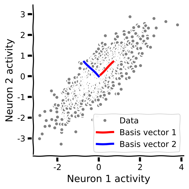
コーディング演習 1.2: 共分散行列の固有ベクトル

次に共分散行列の固有ベクトルを計算します。データと一緒にプロットして、固有ベクトルがデータの形状に合っているか確認しましょう。

手順:

サンプル共分散行列の固有値と固有ベクトルを計算します。（ヒント: 対称行列の固有値を求めるnp.linalg.eighを使いましょう）
固有値を降順に並べ替えるために提供されたコードを使います。
関数plot_basis_vectorsを使って、データの散布図上に固有ベクトルをプロットします。

help(sort_evals_descending)

#################################################
## TODO for students
# Fill out function and remove
raise NotImplementedError("Student exercise: calculate and sort eigenvalues")
#################################################

# Calculate the eigenvalues and eigenvectors
evals, evectors = ...

# Sort the eigenvalues in descending order
evals, evectors = ...

# Visualize
plot_basis_vectors(X, evectors)

解答を見る$

出力例:

# @title Submit your feedback
content_review(f"{feedback_prefix}_Eigenvectors_of_the_covariance_matrix_Exercise")

セクション 2: 固有ベクトルへのデータ射影による主成分分析（PCA）の実行

チュートリアル開始からここまでの推定所要時間: 25分

PCAを実行するには、共分散行列の固有ベクトルにデータを射影します。すなわち、

\bf S = X W

ここで、 $\bf S$ は射影されたデータ（スコアとも呼ばれる）を表す $N_\text{samples} \times N$ 行列であり、 $\bf W$ は共分散行列の固有ベクトル（重みまたは負荷量とも呼ばれる）を各列に持つ $N\times N$ の直交行列です。

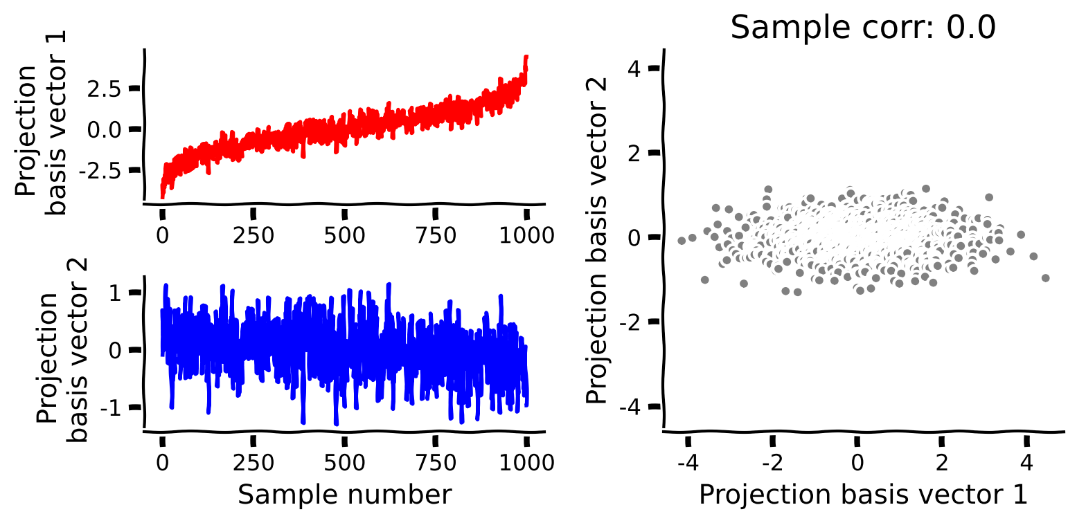
コーディング演習 2: PCAの実装

これまでに得た直感と関数を使って、データに対してPCAを実行します。以下の関数を完成させて、共分散行列の固有ベクトルへのデータ射影によるPCAの手順を実行してください。

手順:

まず平均を引き、標本共分散行列を計算します。
次に固有値と固有ベクトルを求め、降順にソートします。
最後に平均中心化したデータを固有ベクトルに射影します。

help(change_of_basis)

def pca(X):
  """
  Sorts eigenvalues and eigenvectors in decreasing order.

  Args:
    X (numpy array of floats): Data matrix each column corresponds to a
                               different random variable

  Returns:
    (numpy array of floats)  : Data projected onto the new basis
    (numpy array of floats)  : Vector of eigenvalues
    (numpy array of floats)  : Corresponding matrix of eigenvectors

  """

  #################################################
  ## TODO for students: calculate the covariance matrix
  # Fill out function and remove
  raise NotImplementedError("Student exercise: sort eigenvalues/eigenvectors!")
  #################################################

  # Calculate the sample covariance matrix
  cov_matrix = ...

  # Calculate the eigenvalues and eigenvectors
  evals, evectors = ...

  # Sort the eigenvalues in descending order
  evals, evectors = ...

  # Project the data onto the new eigenvector basis
  score = ...

  return score, evectors, evals


# Perform PCA on the data matrix X
score, evectors, evals = pca(X)

# Plot the data projected into the new basis
plot_data_new_basis(score)

解答を見る$

出力例:

# @title Submit your feedback
content_review(f"{feedback_prefix}_PCA_implementation_Exercise")

最後に、共分散行列の固有値を調べます。各固有値は対応する固有ベクトルに射影されたデータの分散を表します。これは重要な概念で、PCAの基底ベクトルをどれだけの分散を捉えられるかでランク付けできることを意味します。まず以下のコードを実行して固有値（「スクリープロット」とも呼ばれます）を描画してください。どちらの固有値が大きいでしょうか？

plot_eigenvalues(evals)

インタラクティブデモ 2: 相関係数の探索

以下のセルを実行し、スライダーを使ってデータの相関係数を変更してください。スクリープロットと基底ベクトルのプロットが更新されるのが見られます。

相関係数を変化させると固有値はどうなりますか？
両方の固有値が等しくなる値を見つけられますか？
片方の固有値だけがゼロでない値を見つけられますか？

# @markdown Make sure you execute this cell to enable the widget!

def refresh(corr_coef=.8):
  cov_matrix = calculate_cov_matrix(variance_1, variance_2, corr_coef)
  X = get_data(cov_matrix)
  score, evectors, evals = pca(X)
  plot_eigenvalues(evals)
  plot_basis_vectors(X, evectors)


_ = widgets.interact(refresh, corr_coef=(-1, 1, .1))

解答を見る$

# @title Submit your feedback
content_review(f"{feedback_prefix}_Exploration_of_the_correlation_coefficient_Interactive_Demo_and_Discussion")

まとめ

チュートリアルの推定所要時間：45分

このチュートリアルでは、PCAの目的はデータの最大分散の方向を捉える直交正規基底を見つけることであることを学びました。より正確には、 $i$ 番目の基底ベクトルは、すべての前の基底ベクトルに直交しながら、射影分散を最大化する方向です。数学的には、これらの基底ベクトルは共分散行列の固有ベクトル（荷重とも呼ばれます）です。
PCAには、射影されたデータ（スコア）が相関しないという有用な性質もあります。
各基底ベクトルに沿った射影分散は対応する固有値で与えられます。これは、各基底ベクトルがデータの変動性をどれだけ説明しているかという「重要度」をランク付けできるため重要です。固有値がゼロであるということは、その方向に変動がないことを意味し、元のデータに関する情報を失うことなくその方向を除外できることを示します。
次のチュートリアルでは、この性質を利用して高次元データの次元削減を行います。

記法

\begin{align}
$\mathbf{x_i}$ & $\quad \text{ニューロン } i \text{ のすべての測定値}$ \
$\bar{\bf x_i}$ & $\quad \text{ニューロン } i \text{ のサンプル平均}$ \
$\bf \Sigma$ & $\quad \text{共分散行列}$ \
$\bf \hat \Sigma$ & $\quad \text{サンプル共分散行列}$ \
$\bf W$ & $\quad \text{重み、荷重行列}$ \
{ $\bf X}$ & $\quad \text{元のデータ行列}$ \
$\bf S$ & $\quad \text{射影行列、スコア}$ \
N & $\quad \text{データの次元数}$ \
N_ $\text{samples}$ & $\quad \text{サンプル数}$ \
\end{align}

ボーナス

ボーナスセクション1：PCAの性質の数学的基礎

# @title Video 2: Properties of PCA
from ipywidgets import widgets
from IPython.display import YouTubeVideo
from IPython.display import IFrame
from IPython.display import display


class PlayVideo(IFrame):
  def __init__(self, id, source, page=1, width=400, height=300, **kwargs):
    self.id = id
    if source == 'Bilibili':
      src = f'https://player.bilibili.com/player.html?bvid={id}&page={page}'
    elif source == 'Osf':
      src = f'https://mfr.ca-1.osf.io/render?url=https://osf.io/download/{id}/?direct%26mode=render'
    super(PlayVideo, self).__init__(src, width, height, **kwargs)


def display_videos(video_ids, W=400, H=300, fs=1):
  tab_contents = []
  for i, video_id in enumerate(video_ids):
    out = widgets.Output()
    with out:
      if video_ids[i][0] == 'Youtube':
        video = YouTubeVideo(id=video_ids[i][1], width=W,
                             height=H, fs=fs, rel=0)
        print(f'Video available at https://youtube.com/watch?v={video.id}')
      else:
        video = PlayVideo(id=video_ids[i][1], source=video_ids[i][0], width=W,
                          height=H, fs=fs, autoplay=False)
        if video_ids[i][0] == 'Bilibili':
          print(f'Video available at https://www.bilibili.com/video/{video.id}')
        elif video_ids[i][0] == 'Osf':
          print(f'Video available at https://osf.io/{video.id}')
      display(video)
    tab_contents.append(out)
  return tab_contents


video_ids = [('Youtube', 'p56UrMRt6-U'), ('Bilibili', 'BV1xa4y1a77c')]
tab_contents = display_videos(video_ids, W=854, H=480)
tabs = widgets.Tab()
tabs.children = tab_contents
for i in range(len(tab_contents)):
  tabs.set_title(i, video_ids[i][0])
display(tabs)

# @title Submit your feedback
content_review(f"{feedback_prefix}_Properties_of_PCA_Bonus_Video")