チュートリアル 1: データの幾何学的視点

第1週, 4日目: 次元削減

Neuromatch Academyによる

コンテンツ制作者: アレックス・カイコ・ガジック、ジョン・マレー

コンテンツレビュアー: ルーズベ・ファルフーディ、マット・クラウス、スピロス・チャヴリス、リチャード・ガオ、マイケル・ワスコム、シッダールト・スレシュ、ナタリー・シャウォロンコウ、エラ・バティ

制作編集者: ガガナ B、スピロス・チャヴリス

チュートリアルの目的

チュートリアルの推定所要時間: 50分

このノートブックでは、多変量データが異なる直交正規基底でどのように表現できるかを探ります。これは次のチュートリアルでPCAを理解するための直感を養うのに役立ちます。

概要:

相関のある多変量データを生成する。
任意の直交正規基底を定義する。
データを新しい基底に射影する。

# @title Tutorial slides
# @markdown These are the slides for the videos in all tutorials today
from IPython.display import IFrame
link_id = "kaq2x"
print(f"If you want to download the slides: https://osf.io/download/{link_id}/")
IFrame(src=f"https://mfr.ca-1.osf.io/render?url=https://osf.io/{link_id}/?direct%26mode=render%26action=download%26mode=render", width=854, height=480)

セットアップ

# @title Install and import feedback gadget


from vibecheck import DatatopsContentReviewContainer
def content_review(notebook_section: str):
    return DatatopsContentReviewContainer(
        "",  # No text prompt
        notebook_section,
        {
            "url": "https://pmyvdlilci.execute-api.us-east-1.amazonaws.com/klab",
            "name": "neuromatch_cn",
            "user_key": "y1x3mpx5",
        },
    ).render()


feedback_prefix = "W1D4_T1"

# Imports
import numpy as np
import matplotlib.pyplot as plt

# @title Figure Settings
import logging
logging.getLogger('matplotlib.font_manager').disabled = True

import ipywidgets as widgets  # interactive display
%config InlineBackend.figure_format = 'retina'
plt.style.use("https://raw.githubusercontent.com/NeuromatchAcademy/course-content/main/nma.mplstyle")

# @title Plotting Functions

def plot_data(X):
  """
  Plots bivariate data. Includes a plot of each random variable, and a scatter
  plot of their joint activity. The title indicates the sample correlation
  calculated from the data.

  Args:
    X (numpy array of floats) : Data matrix each column corresponds to a
                                different random variable

  Returns:
    Nothing.
  """

  fig = plt.figure(figsize=[8, 4])
  gs = fig.add_gridspec(2, 2)
  ax1 = fig.add_subplot(gs[0, 0])
  ax1.plot(X[:, 0], color='k')
  plt.ylabel('Neuron 1')
  plt.title(f'Sample var 1: {np.var(X[:, 0]):.1f}')
  ax1.set_xticklabels([])
  ax2 = fig.add_subplot(gs[1, 0])
  ax2.plot(X[:, 1], color='k')
  plt.xlabel('Sample Number')
  plt.ylabel('Neuron 2')
  plt.title(f'Sample var 2: {np.var(X[:, 1]):.1f}')
  ax3 = fig.add_subplot(gs[:, 1])
  ax3.plot(X[:, 0], X[:, 1], '.', markerfacecolor=[.5, .5, .5],
           markeredgewidth=0)
  ax3.axis('equal')
  plt.xlabel('Neuron 1 activity')
  plt.ylabel('Neuron 2 activity')
  plt.title(f'Sample corr: {np.corrcoef(X[:, 0], X[:, 1])[0, 1]:.1f}')
  plt.show()


def plot_basis_vectors(X, W):
  """
  Plots bivariate data as well as new basis vectors.

  Args:
    X (numpy array of floats) : Data matrix each column corresponds to a
                                different random variable
    W (numpy array of floats) : Square matrix representing new orthonormal
                                basis each column represents a basis vector

  Returns:
    Nothing.
  """

  plt.figure(figsize=[4, 4])
  plt.plot(X[:, 0], X[:, 1], '.', color=[.5, .5, .5], label='Data')
  plt.axis('equal')
  plt.xlabel('Neuron 1 activity')
  plt.ylabel('Neuron 2 activity')
  plt.plot([0, W[0, 0]], [0, W[1, 0]], color='r', linewidth=3,
           label='Basis vector 1')
  plt.plot([0, W[0, 1]], [0, W[1, 1]], color='b', linewidth=3,
           label='Basis vector 2')
  plt.legend()
  plt.show()


def plot_data_new_basis(Y):
  """
  Plots bivariate data after transformation to new bases.
  Similar to plot_data but with colors corresponding to projections onto
  basis 1 (red) and basis 2 (blue). The title indicates the sample correlation
  calculated from the data.

  Note that samples are re-sorted in ascending order for the first
  random variable.

  Args:
    Y (numpy array of floats) : Data matrix in new basis each column
                                corresponds to a different random variable

  Returns:
    Nothing.
  """
  fig = plt.figure(figsize=[8, 4])
  gs = fig.add_gridspec(2, 2)
  ax1 = fig.add_subplot(gs[0, 0])
  ax1.plot(Y[:, 0], 'r')
  plt.xlabel
  plt.ylabel('Projection \n basis vector 1')
  plt.title(f'Sample var 1: {np.var(Y[:, 0]):.1f}')
  ax1.set_xticklabels([])
  ax2 = fig.add_subplot(gs[1, 0])
  ax2.plot(Y[:, 1], 'b')
  plt.xlabel('Sample number')
  plt.ylabel('Projection \n basis vector 2')
  plt.title(f'Sample var 2: {np.var(Y[:, 1]):.1f}')
  ax3 = fig.add_subplot(gs[:, 1])
  ax3.plot(Y[:, 0], Y[:, 1], '.', color=[.5, .5, .5])
  ax3.axis('equal')
  plt.xlabel('Projection basis vector 1')
  plt.ylabel('Projection basis vector 2')
  plt.title(f'Sample corr: {np.corrcoef(Y[:, 0], Y[:, 1])[0, 1]:.1f}')
  plt.show()

# @title Video 1: Geometric view of data
from ipywidgets import widgets
from IPython.display import YouTubeVideo
from IPython.display import IFrame
from IPython.display import display


class PlayVideo(IFrame):
  def __init__(self, id, source, page=1, width=400, height=300, **kwargs):
    self.id = id
    if source == 'Bilibili':
      src = f'https://player.bilibili.com/player.html?bvid={id}&page={page}'
    elif source == 'Osf':
      src = f'https://mfr.ca-1.osf.io/render?url=https://osf.io/download/{id}/?direct%26mode=render'
    super(PlayVideo, self).__init__(src, width, height, **kwargs)


def display_videos(video_ids, W=400, H=300, fs=1):
  tab_contents = []
  for i, video_id in enumerate(video_ids):
    out = widgets.Output()
    with out:
      if video_ids[i][0] == 'Youtube':
        video = YouTubeVideo(id=video_ids[i][1], width=W,
                             height=H, fs=fs, rel=0)
        print(f'Video available at https://youtube.com/watch?v={video.id}')
      else:
        video = PlayVideo(id=video_ids[i][1], source=video_ids[i][0], width=W,
                          height=H, fs=fs, autoplay=False)
        if video_ids[i][0] == 'Bilibili':
          print(f'Video available at https://www.bilibili.com/video/{video.id}')
        elif video_ids[i][0] == 'Osf':
          print(f'Video available at https://osf.io/{video.id}')
      display(video)
    tab_contents.append(out)
  return tab_contents


video_ids = [('Youtube', 'THu9yHnpq9I'), ('Bilibili', 'BV1Af4y1R78w')]
tab_contents = display_videos(video_ids, W=854, H=480)
tabs = widgets.Tab()
tabs.children = tab_contents
for i in range(len(tab_contents)):
  tabs.set_title(i, video_ids[i][0])
display(tabs)

# @title Submit your feedback
content_review(f"{feedback_prefix}_Geometric_view_of_data_Video")

セクション1: 相関のある多変量データを生成する

# @title Video 2: Multivariate data
from ipywidgets import widgets
from IPython.display import YouTubeVideo
from IPython.display import IFrame
from IPython.display import display


class PlayVideo(IFrame):
  def __init__(self, id, source, page=1, width=400, height=300, **kwargs):
    self.id = id
    if source == 'Bilibili':
      src = f'https://player.bilibili.com/player.html?bvid={id}&page={page}'
    elif source == 'Osf':
      src = f'https://mfr.ca-1.osf.io/render?url=https://osf.io/download/{id}/?direct%26mode=render'
    super(PlayVideo, self).__init__(src, width, height, **kwargs)


def display_videos(video_ids, W=400, H=300, fs=1):
  tab_contents = []
  for i, video_id in enumerate(video_ids):
    out = widgets.Output()
    with out:
      if video_ids[i][0] == 'Youtube':
        video = YouTubeVideo(id=video_ids[i][1], width=W,
                             height=H, fs=fs, rel=0)
        print(f'Video available at https://youtube.com/watch?v={video.id}')
      else:
        video = PlayVideo(id=video_ids[i][1], source=video_ids[i][0], width=W,
                          height=H, fs=fs, autoplay=False)
        if video_ids[i][0] == 'Bilibili':
          print(f'Video available at https://www.bilibili.com/video/{video.id}')
        elif video_ids[i][0] == 'Osf':
          print(f'Video available at https://osf.io/{video.id}')
      display(video)
    tab_contents.append(out)
  return tab_contents


video_ids = [('Youtube', 'jcTq2PgU5Vw'), ('Bilibili', 'BV1xz4y1D7ES')]
tab_contents = display_videos(video_ids, W=854, H=480)
tabs = widgets.Tab()
tabs.children = tab_contents
for i in range(len(tab_contents)):
  tabs.set_title(i, video_ids[i][0])
display(tabs)

このビデオでは共分散行列と多変量正規分布について説明しています。

ビデオのテキスト要約はこちらをクリック

直感を得るために、まず単純なモデルを使って多変量データを生成します。具体的には、二変量正規分布からランダムサンプルを引きます。これは1次元の正規分布を2次元に拡張したもので、各 $x_i$ は平均 $\mu_i$ 、分散 $\sigma_i^2$ の周辺正規分布に従います:

x_i \sim \mathcal{N}(\mu_i,\sigma_i^2).

さらに、 $x_1$ と $x_2$ の結合分布には相関係数 $\rho$ が指定されています。相関係数は共分散を正規化したもので、-1から+1の範囲を取ります:

\rho = \frac{\text{cov}(x_1, x_2)}{\sqrt{\sigma_1^2 \sigma_2^2}}.

簡単のため、各変数の平均はすでに差し引かれていると仮定し、 $\mu_i=0$ （ $i=1,2$ ）とします。残りのパラメータは共分散行列にまとめられ、2次元の場合は次の形になります:

{\bf \Sigma} = \begin{pmatrix} \text{var}(x_1) & \text{cov}(x_1,x_2) \\ \text{cov}(x_1,x_2) &\text{var}(x_2) \end{pmatrix}.

一般に、 $\bf \Sigma$ は対称行列で、対角成分に分散 $\text{var}(x_i) = \sigma_i^2$ 、非対角成分に共分散が入ります。後ほど、共分散行列がPCAで重要な役割を果たすことを見ていきます。

# @title Submit your feedback
content_review(f"{feedback_prefix}_Multivariate_data_Video")

コーディング演習1: 分布からサンプルを描く

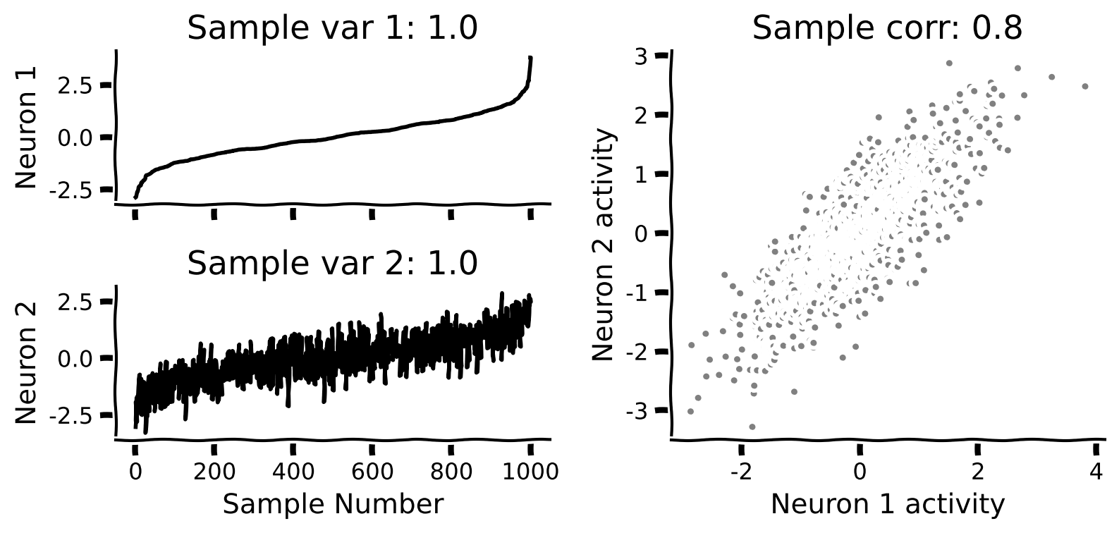
ゼロ平均の二変量正規分布から指定した共分散行列でランダムサンプルを描くコード（get_data）を用意しました。このチュートリアルを通じて、これらのサンプルは異なる試行における2つの記録ニューロンの活動（発火率）を表すと想定します。以下の関数を完成させて、指定した分散と相関係数から共分散行列を計算してください。共分散は上記の式を変形して求められます:

\text{cov}(x_1,x_2) = \rho \sqrt{\sigma_1^2 \sigma_2^2}.

# @markdown Execute this cell to get helper function `get_data`

def get_data(cov_matrix):
  """
  Returns a matrix of 1000 samples from a bivariate, zero-mean Gaussian.

  Note that samples are sorted in ascending order for the first random variable

  Args:
    cov_matrix (numpy array of floats): desired covariance matrix

  Returns:
    (numpy array of floats) : samples from the bivariate Gaussian, with each
                              column corresponding to a different random
                              variable
  """

  mean = np.array([0, 0])
  X = np.random.multivariate_normal(mean, cov_matrix, size=1000)
  indices_for_sorting = np.argsort(X[:, 0])
  X = X[indices_for_sorting, :]

  return X

help(get_data)

def calculate_cov_matrix(var_1, var_2, corr_coef):
  """
  Calculates the covariance matrix based on the variances and correlation
  coefficient.

  Args:
    var_1 (scalar)          : variance of the first random variable
    var_2 (scalar)          : variance of the second random variable
    corr_coef (scalar)      : correlation coefficient

  Returns:
    (numpy array of floats) : covariance matrix
  """

  #################################################
  ## TODO for students: calculate the covariance matrix
  # Fill out function and remove
  raise NotImplementedError("Student exercise: calculate the covariance matrix!")
  #################################################

  # Calculate the covariance from the variances and correlation
  cov = ...

  cov_matrix = np.array([[var_1, cov], [cov, var_2]])

  return cov_matrix


# Set parameters
np.random.seed(2020)  # set random seed
variance_1 = 1
variance_2 = 1
corr_coef = 0.8

# Compute covariance matrix
cov_matrix = calculate_cov_matrix(variance_1, variance_2, corr_coef)

# Generate data with this covariance matrix
X = get_data(cov_matrix)

# Visualize
plot_data(X)

解答を見る$

出力例:

# @title Submit your feedback
content_review(f"{feedback_prefix}_Draw_samples_from_a_distribution_Exercise")

インタラクティブデモ1: 相関のデータへの影響

先ほど完成させた関数を使いますが、今回はスライダーで相関係数を変えられます。相関係数を変えるとシミュレーションデータの幾何学的形状がどう変わるかを体感してください。

負の相関係数の値はどんな影響を与えますか？
どの相関係数の値でデータの分布が円形になりますか？

なお、サンプルはニューロン1の発火率でソートしているため、ニューロン1の発火率のサンプル番号に対するプロットはきれいでほとんど変化がありませんが、ニューロン2はそうではありません。

# @markdown Execute this cell to enable widget

def _calculate_cov_matrix(var_1, var_2, corr_coef):

  # Calculate the covariance from the variances and correlation
  cov = corr_coef * np.sqrt(var_1 * var_2)

  cov_matrix = np.array([[var_1, cov], [cov, var_2]])

  return cov_matrix


@widgets.interact(corr_coef = widgets.FloatSlider(value=.2, min=-1, max=1, step=0.1))
def visualize_correlated_data(corr_coef=0):
  variance_1 = 1
  variance_2 = 1

  # Compute covariance matrix
  cov_matrix = _calculate_cov_matrix(variance_1, variance_2, corr_coef)

  # Generate data with this covariance matrix
  X = get_data(cov_matrix)

  # Visualize
  plot_data(X)

解答を見る$

# @title Submit your feedback
content_review(f"{feedback_prefix}_Correlation_effect_on_data_Interactive_Demo_and_Discussion")

セクション2: 新しい直交正規基底を定義する

ここまでの推定所要時間: 20分

# @title Video 3: Orthonormal bases
from ipywidgets import widgets
from IPython.display import YouTubeVideo
from IPython.display import IFrame
from IPython.display import display


class PlayVideo(IFrame):
  def __init__(self, id, source, page=1, width=400, height=300, **kwargs):
    self.id = id
    if source == 'Bilibili':
      src = f'https://player.bilibili.com/player.html?bvid={id}&page={page}'
    elif source == 'Osf':
      src = f'https://mfr.ca-1.osf.io/render?url=https://osf.io/download/{id}/?direct%26mode=render'
    super(PlayVideo, self).__init__(src, width, height, **kwargs)


def display_videos(video_ids, W=400, H=300, fs=1):
  tab_contents = []
  for i, video_id in enumerate(video_ids):
    out = widgets.Output()
    with out:
      if video_ids[i][0] == 'Youtube':
        video = YouTubeVideo(id=video_ids[i][1], width=W,
                             height=H, fs=fs, rel=0)
        print(f'Video available at https://youtube.com/watch?v={video.id}')
      else:
        video = PlayVideo(id=video_ids[i][1], source=video_ids[i][0], width=W,
                          height=H, fs=fs, autoplay=False)
        if video_ids[i][0] == 'Bilibili':
          print(f'Video available at https://www.bilibili.com/video/{video.id}')
        elif video_ids[i][0] == 'Osf':
          print(f'Video available at https://osf.io/{video.id}')
      display(video)
    tab_contents.append(out)
  return tab_contents


video_ids = [('Youtube', 'PC1RZELnrIg'), ('Bilibili', 'BV1wT4y1E71g')]
tab_contents = display_videos(video_ids, W=854, H=480)
tabs = widgets.Tab()
tabs.children = tab_contents
for i in range(len(tab_contents)):
  tabs.set_title(i, video_ids[i][0])
display(tabs)

# @title Submit your feedback
content_review(f"{feedback_prefix}_Orthonormal_Bases_Video")

このビデオでは、データが異なる基底を使って多様に表現できることを示し、お気に入りの基底が直交正規かどうかを確認する方法を説明しています。

ビデオのテキスト要約はこちらをクリック

次に、新しい直交正規基底ベクトル ${\bf u} = [u_1,u_2]$ と ${\bf w} = [w_1,w_2]$ を定義します。ビデオで学んだように、2つのベクトルが直交正規である条件は:

直交している（つまり内積がゼロ）:

{\bf u\cdot w} = u_1 w_1 + u_2 w_2 = 0

単位長さである:

||{\bf u}|| = ||{\bf w} || = 1

2次元では、任意の直交正規基底を簡単に作れます。まずランダムなベクトル ${\bf u}$ を正規化します。次に第2の基底ベクトルを ${\bf w} = [-u_2,u_1]$ と定義すると、両方の条件が満たされます:

{\bf u\cdot w} = - u_1 u_2 + u_2 u_1 = 0

かつ

{|| {\bf w} ||} = \sqrt{(-u_2)^2 + u_1^2} = \sqrt{u_1^2 + u_2^2} = 1,

ここで ${\bf u}$ が正規化されていることを使いました。したがって、任意の入力ベクトルから直交正規基底を定義でき、基底ベクトルを横に並べた行列で表せます:

{{\bf W} } = \begin{pmatrix} u_1 & w_1 \\ u_2 & w_2 \end{pmatrix}.

コーディング演習2: 直交正規基底を見つける

この演習では、任意の2次元ベクトルを入力として受け取り、直交正規基底を定義する関数を完成させます。

手順

関数 define_orthonormal_basis を修正し、まず第1基底ベクトル $\bf u$ を正規化してください。
次に、 $\bf u$ に直交する基底ベクトル $\bf w$ を見つけて関数を完成させてください。
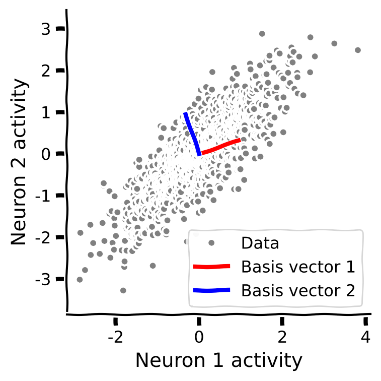
初期基底ベクトル ${\bf u} = [3,1]$ を使って関数をテストし、plot_basis_vectors 関数でデータ散布図の上に基底ベクトルをプロットしてください。（データは $\sigma_1^2 =1$ , $\sigma_2^2 =1$ , $\rho = .8$ を使用）

def define_orthonormal_basis(u):
  """
  Calculates an orthonormal basis given an arbitrary vector u.

  Args:
    u (numpy array of floats) : arbitrary 2-dimensional vector used for new
                                basis

  Returns:
    (numpy array of floats)   : new orthonormal basis
                                columns correspond to basis vectors
  """

  #################################################
  ## TODO for students: calculate the orthonormal basis
  # Fill out function and remove
  raise NotImplementedError("Student exercise: implement the orthonormal basis function")
  #################################################

  # Normalize vector u
  u = ...

  # Calculate vector w that is orthogonal to u
  w = ...

  # Put in matrix form
  W = np.column_stack([u, w])

  return W


# Set up parameters
np.random.seed(2020)  # set random seed
variance_1 = 1
variance_2 = 1
corr_coef = 0.8
u = np.array([3, 1])

# Compute covariance matrix
cov_matrix = calculate_cov_matrix(variance_1, variance_2, corr_coef)

# Generate data
X = get_data(cov_matrix)

# Get orthonomal basis
W = define_orthonormal_basis(u)

# Visualize
plot_basis_vectors(X, W)

解答を見る$

出力例:

# @title Submit your feedback
content_review(f"{feedback_prefix}_Find_an_orthonormal_basis_Exercise")

セクション3: データを新しい基底に射影する

ここまでの推定所要時間: 35分

# @title Video 4: Change of basis
from ipywidgets import widgets
from IPython.display import YouTubeVideo
from IPython.display import IFrame
from IPython.display import display


class PlayVideo(IFrame):
  def __init__(self, id, source, page=1, width=400, height=300, **kwargs):
    self.id = id
    if source == 'Bilibili':
      src = f'https://player.bilibili.com/player.html?bvid={id}&page={page}'
    elif source == 'Osf':
      src = f'https://mfr.ca-1.osf.io/render?url=https://osf.io/download/{id}/?direct%26mode=render'
    super(PlayVideo, self).__init__(src, width, height, **kwargs)


def display_videos(video_ids, W=400, H=300, fs=1):
  tab_contents = []
  for i, video_id in enumerate(video_ids):
    out = widgets.Output()
    with out:
      if video_ids[i][0] == 'Youtube':
        video = YouTubeVideo(id=video_ids[i][1], width=W,
                             height=H, fs=fs, rel=0)
        print(f'Video available at https://youtube.com/watch?v={video.id}')
      else:
        video = PlayVideo(id=video_ids[i][1], source=video_ids[i][0], width=W,
                          height=H, fs=fs, autoplay=False)
        if video_ids[i][0] == 'Bilibili':
          print(f'Video available at https://www.bilibili.com/video/{video.id}')
        elif video_ids[i][0] == 'Osf':
          print(f'Video available at https://osf.io/{video.id}')
      display(video)
    tab_contents.append(out)
  return tab_contents


video_ids = [('Youtube', 'Mj6BRQPKKUc'), ('Bilibili', 'BV1LK411J7NQ')]
tab_contents = display_videos(video_ids, W=854, H=480)
tabs = widgets.Tab()
tabs.children = tab_contents
for i in range(len(tab_contents)):
  tabs.set_title(i, video_ids[i][0])
display(tabs)

# @title Submit your feedback
content_review(f"{feedback_prefix}_Change_of_basis_Video")

最後に、先ほど見つけた新しい基底でデータを表現します。 $\bf W$ は直交正規なので、単純な行列積でデータを新基底に射影できます:

{\bf Y = X W}.

基底の選び方を変えながら、変換後のデータ $\bf Y$ の幾何学的性質を探ります。

コーディング演習3: 直交正規基底への変換

この演習では、データを新しい基底に変換する関数を完成させます。

手順

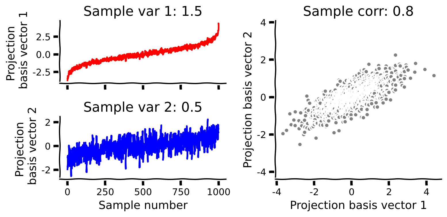
関数 change_of_basis を完成させて、データを新しい基底に射影してください。
plot_data_new_basis 関数で射影後のデータをプロットしてください。
新しい基底での相関係数はどうなりますか？増加しますか、それとも減少しますか？
分散はどうなりますか？

def change_of_basis(X, W):
  """
  Projects data onto new basis W.

  Args:
    X (numpy array of floats) : Data matrix each column corresponding to a
                                different random variable
    W (numpy array of floats) : new orthonormal basis columns correspond to
                                basis vectors

  Returns:
    (numpy array of floats)    : Data matrix expressed in new basis
  """

  #################################################
  ## TODO for students: project the data onto a new basis W
  # Fill out function and remove
  raise NotImplementedError("Student exercise: implement change of basis")
  #################################################

  # Project data onto new basis described by W
  Y = ...

  return Y


# Project data to new basis
Y = change_of_basis(X, W)

# Visualize
plot_data_new_basis(Y)

解答を見る$

出力例:

# @title Submit your feedback
content_review(f"{feedback_prefix}_Change_to_orthonormal_basis_Exercise")

インタラクティブデモ3: 基底ベクトルを操作する

基底ベクトルを変えると相関がどう変わるかを見るため、以下のセルを実行してください。パラメータ $\theta$ は $\bf u$ の角度（度数）を制御します。スライダーで基底ベクトルを回転させてみましょう。

基底を回転させると射影データはどう変わりますか？
相関係数はどう変わりますか？各基底ベクトルへの射影の分散はどう変わりますか？
射影データが無相関になる基底を見つけられますか？

# @markdown Make sure you execute this cell to enable the widget!

def refresh(theta=0):
  u = np.array([1, np.tan(theta * np.pi / 180)])
  W = define_orthonormal_basis(u)
  Y = change_of_basis(X, W)
  plot_basis_vectors(X, W)
  plot_data_new_basis(Y)


_ = widgets.interact(refresh, theta=(0, 90, 5))

解答を見る$

# @title Submit your feedback
content_review(f"{feedback_prefix}_Play_with_basis_vectors_Interactive_Demo_and_Discussion")

まとめ

チュートリアルの推定所要時間: 50分

このチュートリアルでは、多変量データは高次元ベクトル空間の点の雲として視覚化でき、その雲の形状は共分散行列によって決まることを学びました。
多変量データは内積を使って新しい直交正規基底で表現できます。これらの新しい基底ベクトルは元の変数の特定の混合を表し、例えば神経科学ではニューロン集団の活性化の異なる比率を表すことがあります。
新しい基底に変換した後の射影データは元のデータと異なる幾何学的性質を持ち、特に点の雲の広がりに沿った基底ベクトルを取るとデータの相関がなくなります。

これらの概念—共分散、射影、直交正規基底—はPCAを理解する上で重要であり、次のチュートリアルの焦点となります。

記法

\begin{align}
$x_i$ & $\quad \text{次元 } i \text{ のデータ点}$ \
$\mu_i$ & $\quad \text{次元 } i \text{ の平均}$ \
$\sigma_i^2$ & $\quad \text{次元 } i \text{ の分散}$ \
$\bf u, \bf w$ & $\quad \text{直交正規基底ベクトル}$ \
$\rho$ & $\quad \text{相関係数}$ \
$\bf \Sigma$ & $\quad \text{共分散行列}$ \
$\bf X$ & $\quad \text{元のデータ行列}$ \
$\bf W$ & $\quad \text{射影行列}$ \
$\bf Y$ & $\quad \text{変換後のデータ}$ \
\end{align}