チュートリアル 1: エンコーディングのためのGLM

第1週 第3日目: 一般化線形モデル

Neuromatch Academyによる

コンテンツ作成者: Pierre-Etienne H. Fiquet, Ari Benjamin, Jakob Macke

コンテンツレビュアー: Davide Valeriani, Alish Dipani, Michael Waskom, Ella Batty

制作編集者: Spiros Chavlis

チュートリアルの目的

推定所要時間: 1時間15分

これは、教師あり学習の基本的な枠組みである一般化線形モデル（GLM）に関する2部構成のシリーズのパート1です。

このチュートリアルでは、網膜神経節細胞のスパイク列を時系列受容野をフィッティングすることでモデル化します。まずは線形ガウスGLM（別名: 最小二乗法回帰モデル）で、次にポアソンGLM（別名: "線形-非線形-ポアソン"モデル）で行います。次のチュートリアルでは、GLMの特別なケースであるロジスティック回帰に拡張し、良好なモデル性能を確保する方法を学びます。

このチュートリアルは、Uzzell & Chichilnisky 2004の網膜神経節細胞スパイク列データを用いて実行するよう設計されています。

謝辞:

• EJ Chichilnisky氏にデータセット提供の感謝を申し上げます。なお、本データはチュートリアル目的のみで提供されており、著者（[email protected]）の明示的な許可なしに配布や出版に使用してはなりません。
• Jonathan Pillow氏に感謝します。本チュートリアルの多くは彼の『神経データの統計モデリングと解析』クラスの演習に触発されています。

# @title Tutorial slides
# @markdown These are the slides for the videos in all tutorials today
from IPython.display import IFrame
link_id = "upyjz"
print(f"If you want to download the slides: https://osf.io/download/{link_id}/")
IFrame(src=f"https://mfr.ca-1.osf.io/render?url=https://osf.io/{link_id}/?direct%26mode=render%26action=download%26mode=render", width=854, height=480)

セットアップ

# @title Install and import feedback gadget


from vibecheck import DatatopsContentReviewContainer
def content_review(notebook_section: str):
    return DatatopsContentReviewContainer(
        "",  # No text prompt
        notebook_section,
        {
            "url": "https://pmyvdlilci.execute-api.us-east-1.amazonaws.com/klab",
            "name": "neuromatch_cn",
            "user_key": "y1x3mpx5",
        },
    ).render()


feedback_prefix = "W1D3_T1"

# Imports
import numpy as np
import matplotlib.pyplot as plt
from scipy.optimize import minimize
from scipy.io import loadmat

# @title Figure settings
import logging
logging.getLogger('matplotlib.font_manager').disabled = True

%matplotlib inline
%config InlineBackend.figure_format = 'retina'
plt.style.use("https://raw.githubusercontent.com/NeuromatchAcademy/course-content/main/nma.mplstyle")

# @title Plotting Functions

def plot_stim_and_spikes(stim, spikes, dt, nt=120):
  """Show time series of stim intensity and spike counts.

  Args:
    stim (1D array): vector of stimulus intensities
    spikes (1D array): vector of spike counts
    dt (number): duration of each time step
    nt (number): number of time steps to plot

  """
  timepoints = np.arange(nt)
  time = timepoints * dt

  f, (ax_stim, ax_spikes) = plt.subplots(
    nrows=2, sharex=True, figsize=(8, 5),
  )
  ax_stim.plot(time, stim[timepoints])
  ax_stim.set_ylabel('Stimulus intensity')

  ax_spikes.plot(time, spikes[timepoints])
  ax_spikes.set_xlabel('Time (s)')
  ax_spikes.set_ylabel('Number of spikes')

  f.tight_layout()
  plt.show()


def plot_glm_matrices(X, y, nt=50):
  """Show X and Y as heatmaps.

  Args:
    X (2D array): Design matrix.
    y (1D or 2D array): Target vector.

  """
  from matplotlib.colors import BoundaryNorm
  from mpl_toolkits.axes_grid1 import make_axes_locatable
  Y = np.c_[y]  # Ensure Y is 2D and skinny

  f, (ax_x, ax_y) = plt.subplots(
    ncols=2,
    figsize=(6, 8),
    sharey=True,
    gridspec_kw=dict(width_ratios=(5, 1)),
  )
  norm = BoundaryNorm([-1, -.2, .2, 1], 256)
  imx = ax_x.pcolormesh(X[:nt], cmap="coolwarm", norm=norm)

  ax_x.set(
    title="X\n(lagged stimulus)",
    xlabel="Time lag (time bins)",
    xticks=[4, 14, 24],
    xticklabels=['-20', '-10', '0'],
    ylabel="Time point (time bins)",
  )
  plt.setp(ax_x.spines.values(), visible=True)

  divx = make_axes_locatable(ax_x)
  caxx = divx.append_axes("right", size="5%", pad=0.1)
  cbarx = f.colorbar(imx, cax=caxx)
  cbarx.set_ticks([-.6, 0, .6])
  cbarx.set_ticklabels(np.sort(np.unique(X)))

  norm = BoundaryNorm(np.arange(y.max() + 1), 256)
  imy = ax_y.pcolormesh(Y[:nt], cmap="magma", norm=norm)
  ax_y.set(
    title="Y\n(spike count)",
    xticks=[]
  )
  ax_y.invert_yaxis()
  plt.setp(ax_y.spines.values(), visible=True)

  divy = make_axes_locatable(ax_y)
  caxy = divy.append_axes("right", size="30%", pad=0.1)
  cbary = f.colorbar(imy, cax=caxy)
  cbary.set_ticks(np.arange(y.max()) + .5)
  cbary.set_ticklabels(np.arange(y.max()))
  plt.show()


def plot_spike_filter(theta, dt, show=True, **kws):
  """Plot estimated weights based on time lag model.

  Args:
    theta (1D array): Filter weights, not including DC term.
    dt (number): Duration of each time bin.
    kws: Pass additional keyword arguments to plot()
    show (boolean): To plt.show or not the plot.
  """
  d = len(theta)
  t = np.arange(-d + 1, 1) * dt

  ax = plt.gca()
  ax.plot(t, theta, marker="o", **kws)
  ax.axhline(0, color=".2", linestyle="--", zorder=1)
  ax.set(
    xlabel="Time before spike (s)",
    ylabel="Filter weight",
  )
  if show:
    plt.show()


def plot_spikes_with_prediction(spikes, predicted_spikes, dt,
                                nt=50, t0=120, **kws):
  """Plot actual and predicted spike counts.

  Args:
    spikes (1D array): Vector of actual spike counts
    predicted_spikes (1D array): Vector of predicted spike counts
    dt (number): Duration of each time bin.
    nt (number): Number of time bins to plot
    t0 (number): Index of first time bin to plot.
    show (boolean): To plt.show or not the plot.
    kws: Pass additional keyword arguments to plot()

  """
  t = np.arange(t0, t0 + nt) * dt

  f, ax = plt.subplots()
  lines = ax.stem(t, spikes[:nt])
  plt.setp(lines, color=".5")
  lines[-1].set_zorder(1)
  kws.setdefault("linewidth", 3)
  yhat, = ax.plot(t, predicted_spikes[:nt], **kws)
  ax.set(
      xlabel="Time (s)",
      ylabel="Spikes",
  )
  ax.yaxis.set_major_locator(plt.MaxNLocator(integer=True))
  ax.legend([lines[0], yhat], ["Spikes", "Predicted"])
  plt.show()

# @title Data retrieval and loading
import os
import hashlib
import requests

fname = "RGCdata.mat"
url = "https://osf.io/mzujs/download"
expected_md5 = "1b2977453020bce5319f2608c94d38d0"

if not os.path.isfile(fname):
  try:
    r = requests.get(url)
  except requests.ConnectionError:
    print("!!! Failed to download data !!!")
  else:
    if r.status_code != requests.codes.ok:
      print("!!! Failed to download data !!!")
    elif hashlib.md5(r.content).hexdigest() != expected_md5:
      print("!!! Data download appears corrupted !!!")
    else:
      with open(fname, "wb") as fid:
        fid.write(r.content)

セクション1: 線形ガウスGLM

# @title Video 1: Linear Gaussian model
from ipywidgets import widgets
from IPython.display import YouTubeVideo
from IPython.display import IFrame
from IPython.display import display


class PlayVideo(IFrame):
  def __init__(self, id, source, page=1, width=400, height=300, **kwargs):
    self.id = id
    if source == 'Bilibili':
      src = f'https://player.bilibili.com/player.html?bvid={id}&page={page}'
    elif source == 'Osf':
      src = f'https://mfr.ca-1.osf.io/render?url=https://osf.io/download/{id}/?direct%26mode=render'
    super(PlayVideo, self).__init__(src, width, height, **kwargs)


def display_videos(video_ids, W=400, H=300, fs=1):
  tab_contents = []
  for i, video_id in enumerate(video_ids):
    out = widgets.Output()
    with out:
      if video_ids[i][0] == 'Youtube':
        video = YouTubeVideo(id=video_ids[i][1], width=W,
                             height=H, fs=fs, rel=0)
        print(f'Video available at https://youtube.com/watch?v={video.id}')
      else:
        video = PlayVideo(id=video_ids[i][1], source=video_ids[i][0], width=W,
                          height=H, fs=fs, autoplay=False)
        if video_ids[i][0] == 'Bilibili':
          print(f'Video available at https://www.bilibili.com/video/{video.id}')
        elif video_ids[i][0] == 'Osf':
          print(f'Video available at https://osf.io/{video.id}')
      display(video)
    tab_contents.append(out)
  return tab_contents


video_ids = [('Youtube', 'Yv89UHeSa9I'), ('Bilibili', 'BV17T4y1E75x')]
tab_contents = display_videos(video_ids, W=854, H=480)
tabs = widgets.Tab()
tabs.children = tab_contents
for i in range(len(tab_contents)):
  tabs.set_title(i, video_ids[i][0])
display(tabs)

# @title Submit your feedback
content_review(f"{feedback_prefix}_Linear_Gaussian_Model_Video")

セクション1.1: 網膜神経節細胞活動データの読み込み

チュートリアル開始からここまでの推定所要時間: 10分

この演習では、2つの輝度値がランダムに切り替わる画面を提示し、網膜の一種のニューロンである網膜神経節細胞（RGC）の応答を記録した実験データを使用します。この種の視覚刺激は「全視野フリッカー」と呼ばれ、約120Hz（すなわち約8msごとに画面が更新）で提示されました。同じ時間ビンを用いて各ニューロンのスパイク数をカウントしています。

ファイルRGCdata.matには3つの変数が含まれています:

• Stim: 各時点の刺激強度。形状は$T \times 1$の配列で、$T=144051$です。

• SpCounts: 2つのON細胞と2つのOFF細胞のビン化されたスパイク数。$144051 \times 4$の配列で、各列は異なる細胞のカウントを示します。

• dtStim: 1つの時間ビンの大きさ（秒単位）。これはスパイク数/秒の単位でモデル出力を計算するために必要です。刺激のフレームレートは1 / dtStimで与えられます。

これらのデータはすべて行列であるMATLAB形式で保存されているため、読み込み時にPython的な表現（1次元配列やスカラー）に変換します。

data = loadmat('RGCdata.mat')  # loadmat is a function in scipy.io
dt_stim = data['dtStim'].item()  # .item extracts a scalar value

# Extract the stimulus intensity
stim = data['Stim'].squeeze()  # .squeeze removes dimensions with 1 element

# Extract the spike counts for one cell
cellnum = 2
spikes = data['SpCounts'][:, cellnum]

# Don't use all of the timepoints in the dataset, for speed
keep_timepoints = 20000
stim = stim[:keep_timepoints]
spikes = spikes[:keep_timepoints]

plot_stim_and_spikesヘルパー関数を使って、刺激強度とスパイク数の時間変化を可視化しましょう。

plot_stim_and_spikes(stim, spikes, dt_stim)

コーディング演習 1.1: デザイン行列の作成

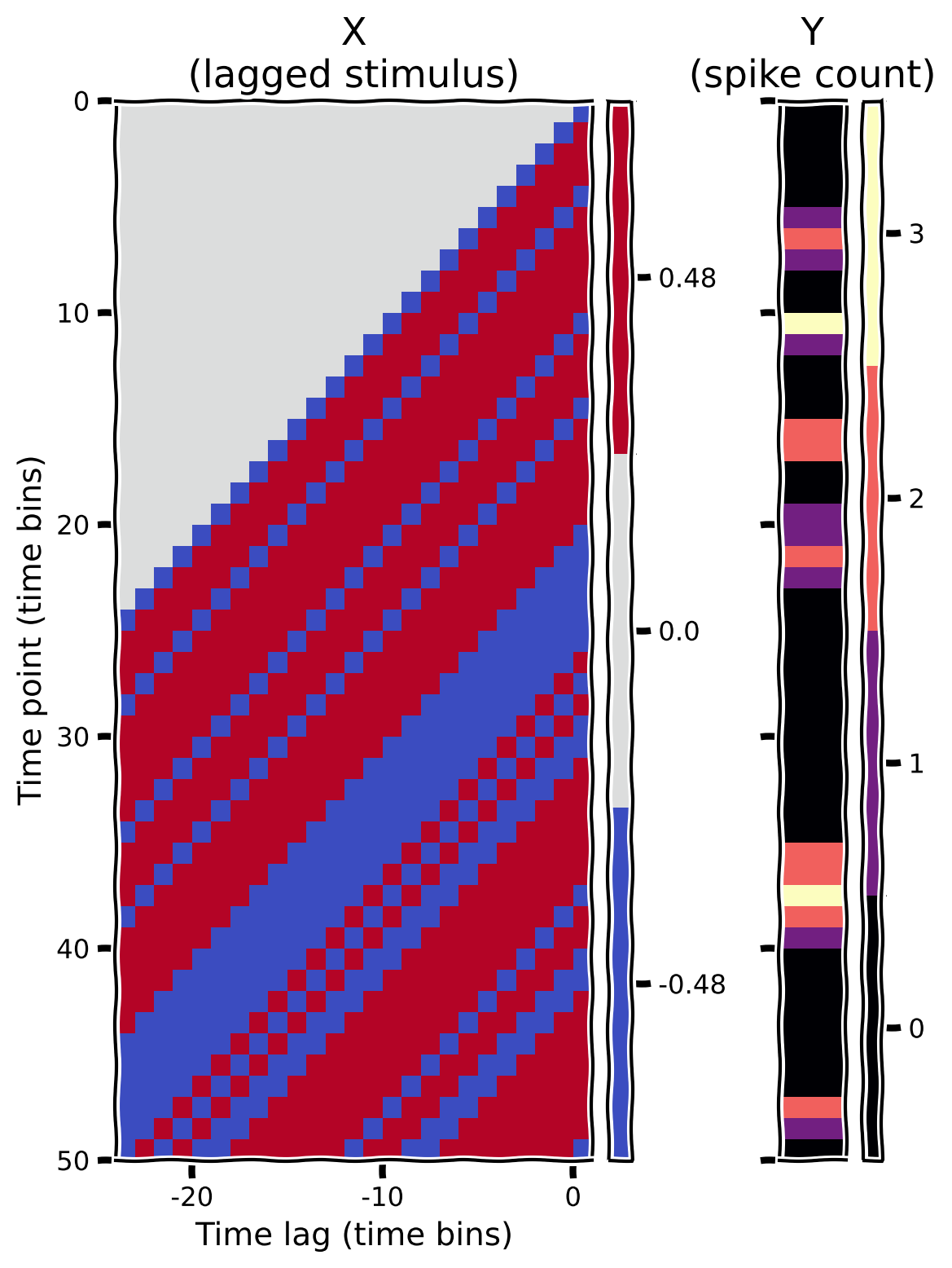
私たちの目標は、細胞の活動をその直前の刺激強度から予測することです。これにより、RGCが時間的にどのように情報を処理しているかを理解できます。そのために、まずこのモデルのデザイン行列を作成します。これは、$i$行目に時点$i$の直前の刺激フレームが並ぶように刺激強度を行列形式で整理したものです。

この演習では、$d=25$の時間遅延を用いてデザイン行列$\mathbf{X}$を作成します。つまり、$\mathbf{X}$は$T \times d$の行列になります。$d=25$（約200ms）は、RGC応答に影響を与える時間窓に関する事前知識に基づく選択です。実際には適切な期間がわからないこともあります。

行tの最後の要素は時刻tに提示された刺激に対応し、その左隣は1つ前の時間ビンの刺激値、という具合です。具体的には、$X_{ij}$は時刻$i + d - 1 - j$の刺激強度となります。

最初の数ビンでは、記録されたスパイク数はありますが、直近の過去の刺激はわかりません。簡単のため、データセットの最初の時点より前の時間遅延に対してはstimの値を0と仮定します。これは「ゼロパディング」と呼ばれ、デザイン行列の行数がspikesの応答ベクトルと同じになるようにします。

以下の関数を完成させてください:

• 刺激のゼロパディング版を作成する
• 正しい形状の空のデザイン行列を初期化する
• ゼロパディング版の刺激を使ってデザイン行列の各行を埋める

デザイン行列（および対応するスパイク数ベクトル）を可視化するために、「ヒートマップ」をプロットします。これは行列の各位置の数値を色で表現するものです。ヘルパー関数にはこれを行うコードが含まれています。

def make_design_matrix(stim, d=25):
  """Create time-lag design matrix from stimulus intensity vector.

  Args:
    stim (1D array): Stimulus intensity at each time point.
    d (number): Number of time lags to use.

  Returns
    X (2D array): GLM design matrix with shape T, d

  """

  # Create version of stimulus vector with zeros before onset
  padded_stim = np.concatenate([np.zeros(d - 1), stim])

  #####################################################################
  # Fill in missing code (...),
  # then remove or comment the line below to test your function
  raise NotImplementedError("Complete the make_design_matrix function")
  #####################################################################


  # Construct a matrix where each row has the d frames of
  # the stimulus preceding and including timepoint t
  T = len(...)  # Total number of timepoints (hint: number of stimulus frames)
  X = np.zeros((T, d))
  for t in range(T):
      X[t] = ...

  return X


# Make design matrix
X = make_design_matrix(stim)

# Visualize
plot_glm_matrices(X, spikes, nt=50)

解答例を見る$

出力例:

# @title Submit your feedback
content_review(f"{feedback_prefix}_Create_design_matrix_Exercise")

セクション1.2: 線形ガウス回帰モデルのフィッティング

チュートリアル開始からここまでの推定所要時間: 25分

まず、デザイン行列を用いて線形ガウスGLM（別名: 一般線形モデル）の最尤推定量を計算します。このモデルのパラメータ$\theta$の最尤推定量は、Day 3で学んだ以下の式で解析的に解けます:

この式を適用する前に、スパイク数はすべて$\geq 0$なので、$y$の平均を考慮するためにデザイン行列を拡張する必要があります。これは、デザイン行列に定数1の列を追加し、モデルが加算的なオフセット重みを学習できるようにします。この追加の重みは$b$（バイアス）と呼びますが、「DC項」や「切片」とも呼ばれます。

# Build the full design matrix
y = spikes
constant = np.ones_like(y)
X = np.column_stack([constant, make_design_matrix(stim)])

# Get the MLE weights for the LG model
theta = np.linalg.inv(X.T @ X) @ X.T @ y
theta_lg = theta[1:]

得られた最尤フィルター推定値（刺激要素に対する25要素の重みベクトル$\theta$のみ、DC項$b$は含まない）をプロットしてください。

plot_spike_filter(theta_lg, dt_stim)

コーディング演習 1.2: 線形ガウスモデルによるスパイク数予測

ここで、これらの要素を組み合わせて、刺激情報から各時点のスパイク数を予測する関数を書きます。

手順は以下の通りです:

• 完全なデザイン行列を作成する
• MLE重み（$\boldsymbol{\hat \theta}$）を取得する
• $\mathbf{\hat y} = \mathbf{X}\boldsymbol{\hat \theta}$を計算する

def predict_spike_counts_lg(stim, spikes, d=25):
  """Compute a vector of predicted spike counts given the stimulus.

  Args:
    stim (1D array): Stimulus values at each timepoint
    spikes (1D array): Spike counts measured at each timepoint
    d (number): Number of time lags to use.

  Returns:
    yhat (1D array): Predicted spikes at each timepoint.

  """
  ##########################################################################
  # Fill in missing code (...) and then comment or remove the error to test
  raise NotImplementedError("Complete the predict_spike_counts_lg function")
  ##########################################################################

  # Create the design matrix
  y = spikes
  constant = ...
  X = ...

  # Get the MLE weights for the LG model
  theta = ...

  # Compute predicted spike counts
  yhat = X @ theta

  return yhat


# Predict spike counts
predicted_counts = predict_spike_counts_lg(stim, spikes)

# Visualize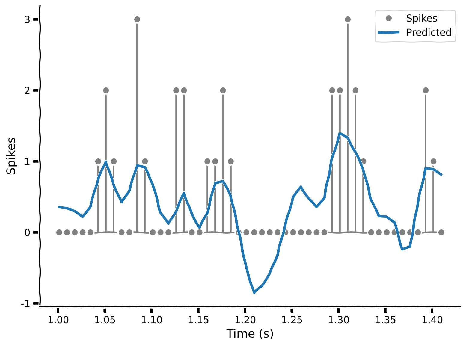
plot_spikes_with_prediction(spikes, predicted_counts, dt_stim)

解答例を見る$

出力例:

# @title Submit your feedback
content_review(f"{feedback_prefix}_Predict_counts_with_Linear_Gaussian_model_Exercise")

このモデルは良いでしょうか？予測線はスパイクの山を大まかに追っていますが、実際に観測されたスパイク数ほど多くは予測しません。さらに問題なのは、一部の時点で負のスパイク数を予測していることです。

ポアソンGLMはこれらの問題を解決するのに役立ちます。

ボーナスチャレンジ

「スパイクトリガー平均（STA）」は線形ガウスGLMの特別な場合として得られます: $\mathrm{STA} = \mathbf{X}^{\top} \mathbf{y} \,/\, \textrm{sum}(\mathbf{y})$。ここで$\mathbf{y}$はニューロンのスパイク数ベクトルです。LG GLMでは、$(\mathbf{X}^{\top}\mathbf{X})^{-1}$の項が回帰子間の相関を補正します。このデータを生成した実験はホワイトノイズ刺激を用いたため、相関はありません。したがって、両者は同等です。（相関がないことをどう確認しますか？）

# @title Submit your feedback
content_review(f"{feedback_prefix}_Bonus_Challenge_Activity")

セクション2: 線形-非線形-ポアソンGLM

チュートリアル開始からここまでの推定所要時間: 36分

# @title Video 2: Generalized linear model
from ipywidgets import widgets
from IPython.display import YouTubeVideo
from IPython.display import IFrame
from IPython.display import display


class PlayVideo(IFrame):
  def __init__(self, id, source, page=1, width=400, height=300, **kwargs):
    self.id = id
    if source == 'Bilibili':
      src = f'https://player.bilibili.com/player.html?bvid={id}&page={page}'
    elif source == 'Osf':
      src = f'https://mfr.ca-1.osf.io/render?url=https://osf.io/download/{id}/?direct%26mode=render'
    super(PlayVideo, self).__init__(src, width, height, **kwargs)


def display_videos(video_ids, W=400, H=300, fs=1):
  tab_contents = []
  for i, video_id in enumerate(video_ids):
    out = widgets.Output()
    with out:
      if video_ids[i][0] == 'Youtube':
        video = YouTubeVideo(id=video_ids[i][1], width=W,
                             height=H, fs=fs, rel=0)
        print(f'Video available at https://youtube.com/watch?v={video.id}')
      else:
        video = PlayVideo(id=video_ids[i][1], source=video_ids[i][0], width=W,
                          height=H, fs=fs, autoplay=False)
        if video_ids[i][0] == 'Bilibili':
          print(f'Video available at https://www.bilibili.com/video/{video.id}')
        elif video_ids[i][0] == 'Osf':
          print(f'Video available at https://osf.io/{video.id}')
      display(video)
    tab_contents.append(out)
  return tab_contents


video_ids = [('Youtube', 'wRbvwdze4uE'), ('Bilibili', 'BV1mz4y1X7JZ')]
tab_contents = display_videos(video_ids, W=854, H=480)
tabs = widgets.Tab()
tabs.children = tab_contents
for i in range(len(tab_contents)):
  tabs.set_title(i, video_ids[i][0])
display(tabs)

# @title Submit your feedback
content_review(f"{feedback_prefix}_Generalized_linear_model_Video")

セクション2.1: scipy.optimizeによる非線形最適化

チュートリアル開始からここまでの推定所要時間: 45分

ポアソンGLMに入る前に、最適化における凸性の重要性と使い方を復習しましょう:

• これまでに、線形ガウスの場合は最尤推定パラメータを解析的に計算できることを見てきました。これはコード1行で済むので非常に便利です！
• 残念ながら、一般には統計推定問題に解析解はなく、非線形最適化アルゴリズムを使って目的関数を最小化するパラメータを探す必要があります。これは、最適解に到達したか局所解にとどまっているかを判定する一般的な方法がないため非常に面倒です。
• この2つの極端の間に、凸目的関数という特別なケースがあります。これは実用上非常に重要で、標準的なソフトウェアを使って非常に信頼性高く（かつ通常は高速に）解くことができます。

補足:

• 関数が凸であるとは、その曲線が任意の2点を結ぶ弦の下側に位置することを意味します。
• 最適化についてもっと学びたい場合は、Stephen BoydとLieven Vandenbergheの書籍Convex Optimizationを参照してください。

ここではscipy.optimizeモジュールを使います。この中のminimize関数は、多数の最適化アルゴリズムに対する汎用的なインターフェースを提供します。この関数は目的関数とパラメータの「初期推定値」を引数に取り、最小関数値、最小値を与えるパラメータ、その他の情報を含む辞書を返します。

簡単な例で動作を見てみましょう。関数$f(x) = x^2$を最小化します:

f = np.square
res = minimize(f, x0=2)
print(f"Minimum value: {res['fun']:.4g} at x = {res['x'].item():.5e}")

$f(x) = x^2$を最小化すると、$x \approx 0$で$f(x) \approx 0$となります。アルゴリズムは「十分近い」最小値で停止するため、厳密に0にはなりません。tolパラメータで「十分近い」の定義を調整できます。

コードのポイントを強調します。minimizeの第一引数は数値や文字列ではなく関数です。ここではnp.squareを使いました。少し珍しいので、何が起きているか理解しておいてください。これは後の演習で重要になります。

この例では初期値$x_0=2$から始めました。異なる初期値で試してみましょう:

start_points = -1, 1.5

xx = np.linspace(-2, 2, 100)
plt.plot(xx, f(xx), color=".2")
plt.xlabel("$x$")
plt.ylabel("$f(x)$")

for i, x0 in enumerate(start_points):
  res = minimize(f, x0)
  plt.plot(x0, f(x0), "o", color=f"C{i}", ms=10, label=f"Start {i}")
  plt.plot(res["x"].item(), res["fun"], "x", c=f"C{i}",
           ms=10, mew=2, label=f"End {i}")
plt.legend()
plt.show()

異なる初期値（点）から始めても、最終的にはほぼ同じ場所（バツ印）に収束します: $f(x_\textrm{final}) \approx 0$。別の関数で試してみましょう:

g = lambda x: x / 5 + np.cos(x)
start_points = -.5, 1.5

xx = np.linspace(-4, 4, 100)
plt.plot(xx, g(xx), color=".2")
plt.xlabel("$x$")
plt.ylabel("$f(x)$")

for i, x0 in enumerate(start_points):
  res = minimize(g, x0)
  plt.plot(x0, g(x0), "o", color=f"C{i}", ms=10, label=f"Start {i}")
  plt.plot(res["x"].item(), res["fun"], "x", color=f"C{i}",
           ms=10, mew=2, label=f"End {i}")
plt.legend()
plt.show()

$f(x) = x^2$とは異なり、$g(x) = \frac{x}{5} + \cos(x)$は凸関数ではありません。最適化の最終位置が初期値に依存するため、問題が複雑になります。

コーディング演習 2.1: ポアソンGLMのフィッティングとスパイク予測

この演習では、scipy.optimize.minimizeを使って、指数非線形性を持つポアソンGLMモデル（LNP: 線形-非線形-ポアソン）のフィルター重みの最尤推定を行います。

実際には2つの関数を完成させます。

• 1つ目は目的関数で、デザイン行列、スパイク数ベクトル、パラメータベクトルを受け取り、負の対数尤度を返します。
• 2つ目はstimとspikesを受け取り、デザイン行列を作成し、内部でminimizeを使ってMLEパラメータを返します。

目的関数は負の対数尤度$-\log P(y \mid \mathbf{X}, \theta)$を返す必要があります。

ポアソンGLMでは、

ここで

全データの対数尤度は:

パラメータ$\theta$に依存しない最後の項は無視してよいので、行列形式で書き直すと:

最後に、負の対数尤度を返すためにマイナス符号を忘れずに。

def neg_log_lik_lnp(theta, X, y):
  """Return -loglike for the Poisson GLM model.

  Args:
    theta (1D array): Parameter vector.
    X (2D array): Full design matrix.
    y (1D array): Data values.

  Returns:
    number: Negative log likelihood.

  """
  #####################################################################
  # Fill in missing code (...), then remove the error
  raise NotImplementedError("Complete the neg_log_lik_lnp function")
  #####################################################################

  # Compute the Poisson log likelihood
  rate = np.exp(X @ theta)
  log_lik = y @ ... - ...

  return ...


def fit_lnp(stim, spikes, d=25):
  """Obtain MLE parameters for the Poisson GLM.

  Args:
    stim (1D array): Stimulus values at each timepoint
    spikes (1D array): Spike counts measured at each timepoint
    d (number): Number of time lags to use.

  Returns:
    1D array: MLE parameters

  """
  #####################################################################
  # Fill in missing code (...), then remove the error
  raise NotImplementedError("Complete the fit_lnp function")
  #####################################################################

  # Build the design matrix
  y = spikes
  constant = np.ones_like(y)
  X = np.column_stack([constant, make_design_matrix(stim)])

  # Use a random vector of weights to start (mean 0, sd .2)
  x0 = np.random.normal(0, .2, d + 1)

  # Find parameters that minimize the negative log likelihood function
  res = minimize(..., args=(X, y))

  return ...


# Fit LNP model
theta_lnp = fit_lnp(stim, spikes)

# Visualize
plot_spike_filter(theta_lg[1:], dt_stim, show=False, color=".5", label="LG")
plot_spike_filter(theta_lnp[1:], dt_stim, show=False, label="LNP")
plt.legend(loc="upper left")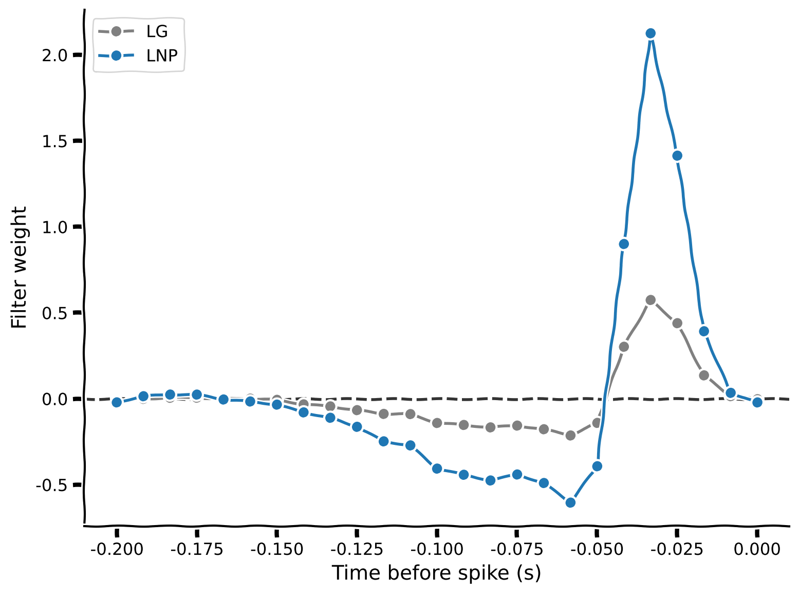
plt.show()

解答例を見る$

出力例:

# @title Submit your feedback
content_review(f"{feedback_prefix}_Fitting_the_Poisson_GLM_Exercise")

LGモデルとLNPモデルの重みを並べてプロットすると、概ね似ていますがLNPの方が一般に大きいです。これはモデルのスパイク予測能力にどう影響するでしょうか？それを見るために、predict_spike_counts_lnp関数を完成させましょう:

def predict_spike_counts_lnp(stim, spikes, theta=None, d=25):
  """Compute a vector of predicted spike counts given the stimulus.

  Args:
    stim (1D array): Stimulus values at each timepoint
    spikes (1D array): Spike counts measured at each timepoint
    theta (1D array): Filter weights; estimated if not provided.
    d (number): Number of time lags to use.

  Returns:
    yhat (1D array): Predicted spikes at each timepoint.

  """
  ###########################################################################
  # Fill in missing code (...) and then remove the error to test
  raise NotImplementedError("Complete the predict_spike_counts_lnp function")
  ###########################################################################

  y = spikes
  constant = np.ones_like(spikes)
  X = np.column_stack([constant, make_design_matrix(stim)])
  if theta is None:  # Allow pre-cached weights, as fitting is slow
    theta = fit_lnp(X, y, d)

  yhat = ...
  return yhat


# Predict spike counts
yhat = predict_spike_counts_lnp(stim, spikes, theta_lnp)

# Visualize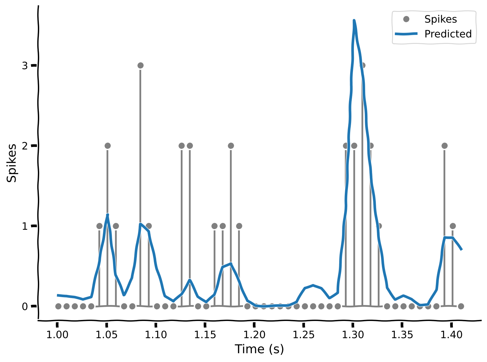
plot_spikes_with_prediction(spikes, yhat, dt_stim)

解答例を見る$

出力例:

# @title Submit your feedback
content_review(f"{feedback_prefix}_Predict_spike_counts_Exercise")

LNPモデルは実際のスパイクデータにより良くフィットしていることがわかります。重要なのは、負のスパイク数を予測しないことです！

ボーナス: LNPモデルが「より良い」と言ったのは定性的で主にプロットの見た目に基づいていますが、これを定量的に示すにはどうすればよいでしょうか？

# @title Submit your feedback
content_review(f"{feedback_prefix}_Predict_spike_counts_Bonus")

まとめ

推定所要時間: 1時間15分

この最初のチュートリアルでは、2つの異なるモデルを使って網膜神経節細胞がフリッカー白色雑音刺激にどう応答するかを学びました。異なるGLMに渡せるデザイン行列の作り方を学び、線形-非線形-ポアソン（LNP）モデルが単純な線形ガウス（LG）モデルよりもスパイク率をより良く予測できることを見ました。

次のチュートリアルでは、さらにこれらのアイデアを拡張します。別のGLMであるロジスティック回帰に出会い、パラメータ数$d$がデータ点数$N$に比べて多い場合でも良好なモデル性能を確保する方法を学びます。

記法

\begin{align}
y &$\quad \text{測定値または応答、ここではスパイク数}$\
T &$\quad \text{時点数}$\
d &$\quad \text{入力の次元数}$\
$\mathbf{X}$ &$\quad \text{デザイン行列、次元: } T \times d$\
$\theta$ &$\quad \text{パラメータ}$\
$\hat \theta$ &$\quad \text{推定されたパラメータ}$\
$\hat y$ &$\quad \text{推定された応答}$\
P($\mathbf{y} \mid \mathbf{X}, \theta)$ &$\quad \text{デザイン行列}\mathbf{X} \text{とパラメータ}\theta \text{のもとで応答} y \text{が観測される確率}$ \
$\mathrm{STA}$ &$\quad \text{スパイクトリガー平均}$\
b &$\quad \text{バイアス重み、切片}$\
\end{align}