チュートリアル 6: モデル選択：クロスバリデーション

第1週、第2日目：モデルフィッティング

Neuromatch Academyによる

コンテンツ作成者: Pierre-Étienne Fiquet、Anqi Wu、Alex Hyafil（Ella Battyの協力を得て）

コンテンツレビュアー: Lina Teichmann、Patrick Mineault、Michael Waskom

制作編集者: Spiros Chavlis

チュートリアルの目的

チュートリアルの推定所要時間：25分

これはデータにモデルをフィットさせるシリーズのチュートリアル6です。最初は単純な線形回帰を、最小二乗法（チュートリアル1）と最尤推定（チュートリアル2）を使って学びました。推定した線形モデルのパラメータの信頼区間をブートストラップで構築する方法も学びました（チュートリアル3）。回帰モデルの探求は、多重線形回帰や多項式回帰への一般化で終わります（チュートリアル4）。最後に、これらの様々なモデルの中からどのモデルを選ぶかを学びます。バイアス・バリアンストレードオフ（チュートリアル5）とモデル選択のためのクロスバリデーション（チュートリアル6）について議論します。

チュートリアルの目的：

クロスバリデーションを実装し、多項式回帰モデルを比較する

# @title Tutorial slides
# @markdown These are the slides for the videos in all tutorials today
from IPython.display import IFrame
link_id = "2mkq4"
print(f"If you want to download the slides: https://osf.io/download/{link_id}/")
IFrame(src=f"https://mfr.ca-1.osf.io/render?url=https://osf.io/{link_id}/?direct%26mode=render%26action=download%26mode=render", width=854, height=480)

セットアップ

# @title Install and import feedback gadget


from vibecheck import DatatopsContentReviewContainer
def content_review(notebook_section: str):
    return DatatopsContentReviewContainer(
        "",  # No text prompt
        notebook_section,
        {
            "url": "https://pmyvdlilci.execute-api.us-east-1.amazonaws.com/klab",
            "name": "neuromatch_cn",
            "user_key": "y1x3mpx5",
        },
    ).render()


feedback_prefix = "W1D2_T6"

# Imports
import numpy as np
import matplotlib.pyplot as plt
from sklearn.model_selection import KFold

# @title Figure Settings
import logging
logging.getLogger('matplotlib.font_manager').disabled = True

%config InlineBackend.figure_format = 'retina'
plt.style.use("https://raw.githubusercontent.com/NeuromatchAcademy/course-content/main/nma.mplstyle")

# @title Plotting Functions

def plot_cross_validate_MSE(mse_all):
  """ Plot the MSE values for the K_fold cross validation

  Args:
    mse_all (ndarray): an array of size (number of splits, max_order + 1)
  """
  plt.figure()
  plt.boxplot(mse_all, labels=np.arange(0, max_order + 1))

  plt.xlabel('Polynomial Order')
  plt.ylabel('Validation MSE')
  plt.title(f'Validation MSE over {n_splits} splits of the data')
  plt.show()


def plot_AIC(order_list, AIC_list):
  """ Plot the AIC value for fitted polynomials of various orders

  Args:
    order_list (list): list of fitted polynomial orders
    AIC_list (list): list of AIC values corresponding to each polynomial model on order_list
  """
  plt.bar(order_list, AIC_list)
  plt.ylabel('AIC')
  plt.xlabel('polynomial order')
  plt.title('comparing polynomial fits')
  plt.show()

# @title Helper Functions

def ordinary_least_squares(x, y):
  """Ordinary least squares estimator for linear regression.

  Args:
    x (ndarray): design matrix of shape (n_samples, n_regressors)
    y (ndarray): vector of measurements of shape (n_samples)

  Returns:
    ndarray: estimated parameter values of shape (n_regressors)
  """

  return np.linalg.inv(x.T @ x) @ x.T @ y


def make_design_matrix(x, order):
  """Create the design matrix of inputs for use in polynomial regression

  Args:
    x (ndarray): input vector of shape (n_samples)
    order (scalar): polynomial regression order

  Returns:
    ndarray: design matrix for polynomial regression of shape (samples, order+1)
  """

  # Broadcast to shape (n x 1)
  if x.ndim == 1:
    x = x[:, None]

  #if x has more than one feature, we don't want multiple columns of ones so we assign
  # x^0 here
  design_matrix = np.ones((x.shape[0], 1))

  # Loop through rest of degrees and stack columns
  for degree in range(1, order + 1):
      design_matrix = np.hstack((design_matrix, x**degree))

  return design_matrix


def solve_poly_reg(x, y, max_order):
  """Fit a polynomial regression model for each order 0 through max_order.

  Args:
    x (ndarray): input vector of shape (n_samples)
    y (ndarray): vector of measurements of shape (n_samples)
    max_order (scalar): max order for polynomial fits

  Returns:
    dict: fitted weights for each polynomial model (dict key is order)
  """

  # Create a dictionary with polynomial order as keys, and np array of theta
  # (weights) as the values
  theta_hats = {}

  # Loop over polynomial orders from 0 through max_order
  for order in range(max_order + 1):

    X = make_design_matrix(x, order)
    this_theta = ordinary_least_squares(X, y)

    theta_hats[order] = this_theta

  return theta_hats


def evaluate_poly_reg(x, y, theta_hats, max_order):
    """ Evaluates MSE of polynomial regression models on data

    Args:
      x (ndarray): input vector of shape (n_samples)
      y (ndarray): vector of measurements of shape (n_samples)
      theta_hat (dict): fitted weights for each polynomial model (dict key is order)
      max_order (scalar): max order of polynomial fit

    Returns
      (ndarray): mean squared error for each order, shape (max_order)
    """

    mse = np.zeros((max_order + 1))
    for order in range(0, max_order + 1):
      X_design = make_design_matrix(x, order)
      y_hat = np.dot(X_design, theta_hats[order])
      residuals = y - y_hat
      mse[order] = np.mean(residuals ** 2)

    return mse

セクション1：クロスバリデーション

# @title Video 1: Cross-Validation
from ipywidgets import widgets
from IPython.display import YouTubeVideo
from IPython.display import IFrame
from IPython.display import display


class PlayVideo(IFrame):
  def __init__(self, id, source, page=1, width=400, height=300, **kwargs):
    self.id = id
    if source == 'Bilibili':
      src = f'https://player.bilibili.com/player.html?bvid={id}&page={page}'
    elif source == 'Osf':
      src = f'https://mfr.ca-1.osf.io/render?url=https://osf.io/download/{id}/?direct%26mode=render'
    super(PlayVideo, self).__init__(src, width, height, **kwargs)


def display_videos(video_ids, W=400, H=300, fs=1):
  tab_contents = []
  for i, video_id in enumerate(video_ids):
    out = widgets.Output()
    with out:
      if video_ids[i][0] == 'Youtube':
        video = YouTubeVideo(id=video_ids[i][1], width=W,
                             height=H, fs=fs, rel=0)
        print(f'Video available at https://youtube.com/watch?v={video.id}')
      else:
        video = PlayVideo(id=video_ids[i][1], source=video_ids[i][0], width=W,
                          height=H, fs=fs, autoplay=False)
        if video_ids[i][0] == 'Bilibili':
          print(f'Video available at https://www.bilibili.com/video/{video.id}')
        elif video_ids[i][0] == 'Osf':
          print(f'Video available at https://osf.io/{video.id}')
      display(video)
    tab_contents.append(out)
  return tab_contents


video_ids = [('Youtube', 'OtKw0rSRxo4'), ('Bilibili', 'BV1mt4y1Q7C4')]
tab_contents = display_videos(video_ids, W=854, H=480)
tabs = widgets.Tab()
tabs.children = tab_contents
for i in range(len(tab_contents)):
  tabs.set_title(i, video_ids[i][0])
display(tabs)

# @title Submit your feedback
content_review(f"{feedback_prefix}_CrossValidation_Video")

特定の問題に対してどのモデルを使うか複数の選択肢があります。線形回帰、2次多項式回帰、3次多項式回帰などです。チュートリアル5で見たように、異なるモデルはトレーニングデータとテストデータの両方で予測の質が異なります。

モデル選択でよく使われる方法は、モデルがまだ見たことのない新しいデータをどれだけよく予測できるかを評価することです。しかし、テストデータを使ってこれを行うと、トレーニング過程でテストデータを使ってしまうことになるので避けたいです。そこで、検証データと呼ばれる別のホールドアウトデータを使います。このデータではモデルをフィットさせず、最良のモデルを選ぶために使います。

ただし、特に神経科学の分野ではデータ量が限られていることが多いため、検証用にデータを割り当ててトレーニングデータをさらに減らしたくありません。幸いなことに、k分割クロスバリデーションを使うことができます。k分割クロスバリデーションでは、トレーニングデータをk個のサブセット（foldと呼びます、下図参照）に分割し、最初のk-1個のfoldでモデルをトレーニングし、最後の1つのfoldで誤差を計算します。このプロセスをk回繰り返し、それぞれ異なるfoldをホールドアウトとして使います。これらk回の各モデル（splitと呼びます、下図参照）は異なるfoldを除外してフィットされます。最後に、各モデルのホールドアウトサブセットでの誤差を平均し、これをモデル選択に使う性能指標とします。

具体的に説明すると、トレーニングデータが1000サンプルあり、4分割クロスバリデーションを選んだとします。サンプル0～250がサブセット1、250～500がサブセット2、500～750がサブセット3、750～1000がサブセット4です。まず、3次多項式回帰モデルをサブセット1、2、3でトレーニングし、サブセット4で評価します。次に、サブセット1、2、4でトレーニングし、サブセット3で評価します。このようにして、4回の3次多項式回帰モデルのトレーニングが行われ、それぞれ異なるサブセットをホールドアウトとして使い、その誤差を平均します。

これで異なるモデルの誤差を比較し、ホールドアウトデータに対してよく一般化するモデルを選べます。予測の質の指標は目的に応じて選べます。ここでは平均二乗誤差（MSE）を使いますが、データの対数尤度なども使えます。

最後に、通常はこのモデルを全トレーニングデータ（サブセット分割なし）で再度トレーニングし、テストデータで評価する最終モデルを得ます。この方法により、貴重なトレーニングデータを犠牲にせずに新しいデータでの予測性能を評価できます。

ホールドアウトサブセットは検証用またはテスト用と呼ばれますが、明確な合意はなく、k分割クロスバリデーションの使い方によって異なります。k分割クロスバリデーションをモデル選択に使い、その後ホールドアウトテストデータで性能を報告する場合もあれば、ホールドアウトサブセットの平均誤差をモデル性能として報告する場合もあります。このテキストとコードでは、完全にホールドアウトされたテストデータと区別するために、ホールドアウトサブセットを検証用サブセットと呼びます（上の動画とは異なります）。

これらのステップはScikit-learnのこの図にまとめられています（https://scikit-learn.org/stable/modules/cross_validation.html）

Sklearnの図 $

重要なのは、データをサブセットに分割する際に非常に注意することです。ホールドアウトサブセットはモデルのフィッティングに一切使ってはいけません。サブセットに分割する前に前処理（例えば正規化）を行うと、ホールドアウトサブセットがトレーニングサブセットに影響を与えてしまう可能性があります。クロスバリデーションでの誤検出の多くは誤った分割から生じます。

モデル選択方法の選択において重要な考慮点は関連するバイアスです。トレーニングデータのMSEだけでフィットすると、パラメータ数を増やすほどフィットが良くなり過学習してしまうことが多いです（チュートリアル5参照）。クロスバリデーションを使う場合、バイアスは逆になります。パラメータ数が多いモデルは分散の影響を受けやすいため、クロスバリデーションは一般にパラメータ数の少ないモデルを好みます。

再びトレーニングデータとテストデータをシミュレートし、多項式回帰モデルをフィットします

# @markdown Execute this cell to simulate data and fit polynomial regression models

# Generate training data
np.random.seed(0)
n_train_samples = 50
x_train = np.random.uniform(-2, 2.5, n_train_samples)  # sample from a uniform distribution over [-2, 2.5)
noise = np.random.randn(n_train_samples)  # sample from a standard normal distribution
y_train = x_train**2 - x_train - 2 + noise

# Generate testing data
n_test_samples = 20
x_test = np.random.uniform(-3, 3, n_test_samples)  # sample from a uniform distribution over [-2, 2.5)
noise = np.random.randn(n_test_samples)  # sample from a standard normal distribution
y_test = x_test**2 - x_test - 2 + noise

# Fit polynomial regression models
max_order = 5
theta_hats = solve_poly_reg(x_train, y_train, max_order)

コーディング演習1：クロスバリデーションの実装

評価するモデル群（0次から5次までの多項式回帰モデル）に対して、クロスバリデーションを使い、新しいデータに対する予測がMSEで最も良いモデルを決定します。

このコードでは、KFold（sklearn.model_selectionから）を使ってデータを10個のサブセットに分割します。KFoldはクロスバリデーションのサブセット分割とトレーニング/検証割り当てを処理します。特に、KFold.splitメソッドはイテレータを返し、ループで回せます。各ループで異なるサブセットを検証用に割り当て、トレーニングと検証のインデックスを返します。

10回のトレーニング/検証スプリットをループし、それぞれで異なる次数の多項式回帰モデルをフィットします。solve_poly_reg（チュートリアル4）とevaluate_poly_reg（チュートリアル5）を使う必要があります（このノートブックに既に実装済みです）。

各多項式次数ごとに10回の検証MSEをボックスプロットで可視化します。

help(solve_poly_reg)

help(evaluate_poly_reg)

def cross_validate(x_train, y_train, max_order, n_splits):
  """ Compute MSE for k-fold validation for each order polynomial

  Args:
    x_train (ndarray): training data input vector of shape (n_samples)
    y_train (ndarray): training vector of measurements of shape (n_samples)
    max_order (scalar): max order of polynomial fit
    n_split (scalar): number of folds for k-fold validation

  Return:
    ndarray: MSE over splits for each model order, shape (n_splits, max_order + 1)

  """

  # Initialize the split method
  kfold_iterator = KFold(n_splits)

  # Initialize np array mse values for all models for each split
  mse_all = np.zeros((n_splits, max_order + 1))

  for i_split, (train_indices, val_indices) in enumerate(kfold_iterator.split(x_train)):

      # Split up the overall training data into cross-validation training and validation sets
      x_cv_train = x_train[train_indices]
      y_cv_train = y_train[train_indices]
      x_cv_val = x_train[val_indices]
      y_cv_val = y_train[val_indices]

      #############################################################################
      ## TODO for students: Fill in missing ... in code below to choose which data
      ## to fit to and compute MSE for
      # Fill out function and remove
      raise NotImplementedError("Student exercise: implement cross-validation")
      #############################################################################

      # Fit models
      theta_hats = ...

      # Compute MSE
      mse_this_split = ...

      mse_all[i_split] = mse_this_split

  return mse_all


# Cross-validate
max_order = 5
n_splits = 10
mse_all = cross_validate(x_train, y_train, max_order, n_splits)

# Visualize
plot_cross_validate_MSE(mse_all)

解答を見る$

出力例:

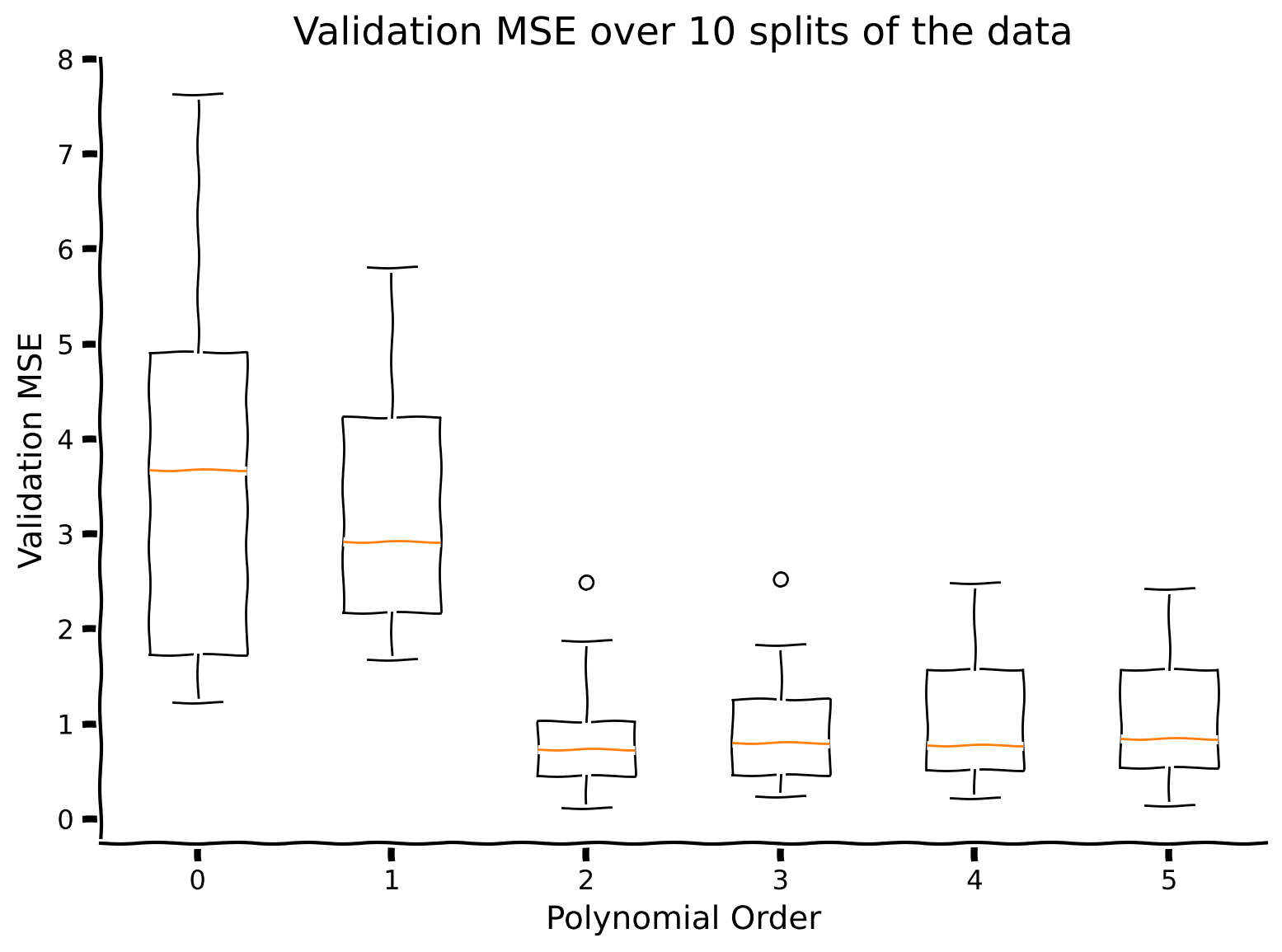
どの多項式の次数がデータのより良いモデルだと思いますか？

# @title Submit your feedback
content_review(f"{feedback_prefix}_Implement_Cross_Validation_Exercise")

まとめ

チュートリアルの推定所要時間: 25分

特定の問題に対して最適なモデルを決定するために、モデル選択の手法を使う必要があります。

交差検証は、モデルが新しいデータをどれだけよく予測できるかに焦点を当てています。

ボーナス

ボーナスセクション1: 赤池情報量規準（AIC）

特定の問題に最適なモデルを選ぶために、与えられたモデルのもとでデータがどれだけ起こりやすいかを考えます。データに高い確率を割り当てるモデルを選びたいのです。このアプローチを用いたモデル選択の一般的な方法が**赤池情報量規準（AIC）**です。

本質的に、AICはモデルの予測を真のデータの代わりに使った場合にどれだけ情報が失われるか（モデルの相対的な情報価値）を推定します。各モデルのAICを計算し、最も低いAICのモデルを選びます。AICは相対的な良さを示すだけで、絶対的にどれだけ良いかはわかりません。

AICはモデルの複雑さと失われる情報量を考慮し、過学習と過小学習の良いバランスを目指します。AICは次のように計算されます。

\mathrm{AIC} = 2K - 2 \log(\mathcal{L})

ここで、 $K$ はモデルのパラメータ数、 $\mathcal{L}$ はモデルが出力データを生成した可能性（尤度）です。

AICが何か分かったので、多項式回帰モデルの中からこれを使って選びたいと思います。ただし、尤度の観点で考えていなかったので、 $\mathcal{L}$ はどう計算すればよいでしょうか？

チュートリアル2で見たように、線形回帰モデルの平均二乗誤差と尤度推定には関連があり、それを利用できます。

導出タイム！

上記のAICの式から始めます。

\mathrm{AIC} = 2k - 2 \log \mathcal{L}

正規誤差を持つモデルの場合、正規分布の対数尤度を使えます。

\log \mathcal{L} = -\frac{n}{2} \log(2 \pi) -\frac{n}{2}\log(\sigma^2) - \sum_i^N \frac{1}{2 \sigma^2} (y_i - \tilde y_i)^2

最初の項は定数なので、AICでの相対情報量の評価には影響しないため省略できます。最後の項も実は定数です： $\sigma^2$ は事前にわからないので、残差からの経験的推定値（ $\hat{\sigma}^2 = 1/N\sum_i^N (y_i - \tilde y_i)^2$ ）を使います。これを代入すると、分子と分母の $\sum [(y - \tilde y)^2]$ の項が打ち消し合い、最後の項は $\frac N 2$ となります。

定数項を省き、AICの式に組み込むと次のようになります。

\mathrm{AIC} = 2k + n\log \left( \sigma^2 \right)

$\sigma^2$ は分散の計算（誤差二乗和をサンプル数で割ったもの）に置き換えられます。したがって、線形回帰や多項式回帰のAICは次の式になります。

\mathrm{AIC} = 2K + n \log \left( \frac{\mathrm{SSE}}{n} \right)

ここで、 $k$ はパラメータ数、 $n$ はサンプル数、 $\mathrm{SSE}$ は誤差二乗和です。

ボーナス演習1: AICを計算しよう

AIC_list = []
order_list = list(range(max_order + 1))

for order in order_list:

  # Compute predictions for this model
  X_design = make_design_matrix(x_train, order)
  y_hat = np.dot(X_design, theta_hats[order])

  #############################################################################
  ## TODO for students:
  ## to fit to and compute MSE for
  # Fill out function and remove
  raise NotImplementedError("Student exercise: implement compute AIC")
  # 1) Compute sum of squared errors (SSE) given prediction y_hat and y_train
  # 2) Identify number of parameters in this model (K in formula above)
  # 3) Compute AIC (call this_AIC) according to formula above
  #############################################################################

  # Compute SSE
  residuals = ...
  sse = ...

  # Get K
  K = len(theta_hats[order])

  # Compute AIC
  AIC = ...

  AIC_list.append(AIC)

# Visualize
plt.bar(order_list, AIC_list)

plt.ylabel('AIC')
plt.xlabel('polynomial order')
plt.title('comparing polynomial fits')
plt.show()

解答を見る$

出力例:

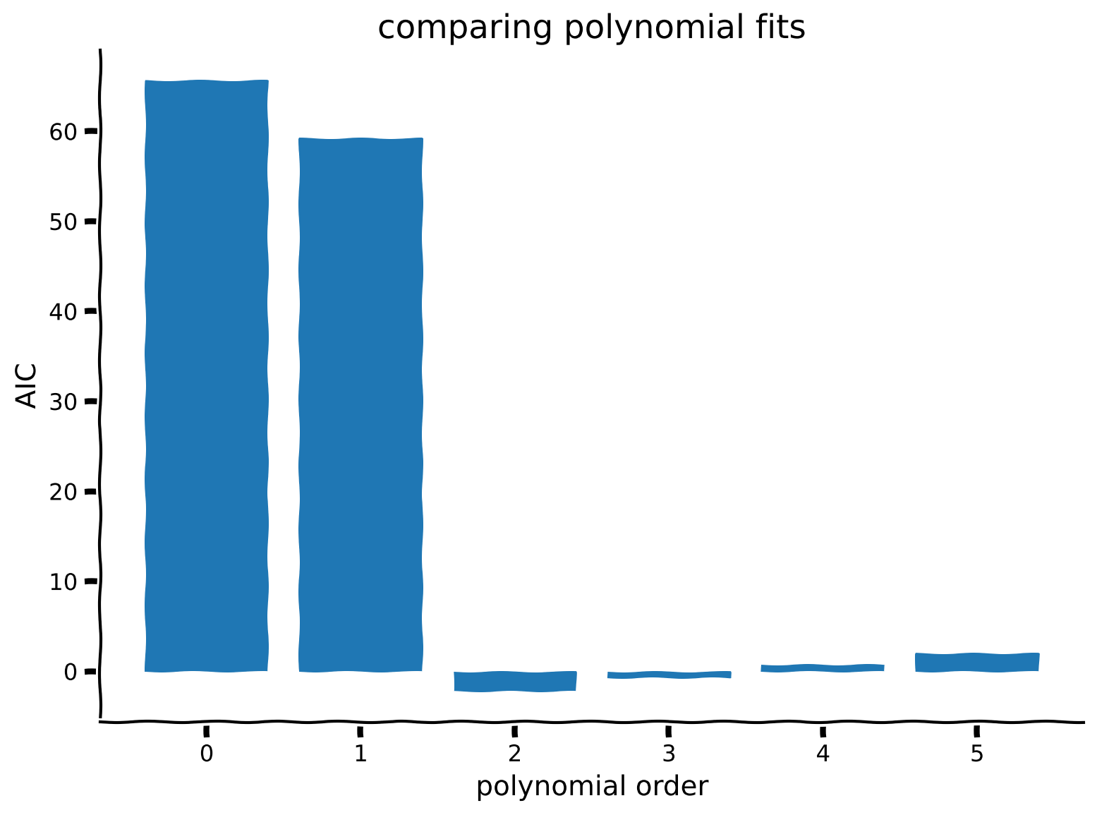
AICに基づくとどのモデルを選びますか？

# @title Submit your feedback
content_review(f"{feedback_prefix}_Compute_AIC_Bonus_Exercise")