チュートリアル 5: モデル選択：バイアス・バリアンストレードオフ

第1週、第2日目：モデルフィッティング

Neuromatch Academyによる

コンテンツ制作者: Pierre-Étienne Fiquet, Anqi Wu, Alex Hyafil（Ella Battyの協力を得て）

コンテンツレビュアー: Lina Teichmann, Patrick Mineault, Michael Waskom

制作編集者: Spiros Chavlis

チュートリアルの目的

推定所要時間: 25分

これはデータにモデルをフィットさせるシリーズのチュートリアル5です。最初に単純な線形回帰を、最小二乗法（チュートリアル1）と最尤推定（チュートリアル2）を使って学びました。推定した線形モデルのパラメータの信頼区間をブートストラップで構築する方法を学びました（チュートリアル3）。回帰モデルの探求は、多重線形回帰と多項式回帰に一般化することで終わりました（チュートリアル4）。最後に、これらの様々なモデルの中から選択する方法を学びます。バイアス・バリアンストレードオフ（チュートリアル5）とモデル選択のための交差検証（チュートリアル6）について議論します。

このチュートリアルでは、バイアス・バリアンストレードオフについて学び、多項式回帰モデルを使ってその動作を確認します。

チュートリアルの目的:

訓練データとテストデータの違いを理解する
複雑さの異なるモデルの訓練誤差とテスト誤差を比較する
バイアス・バリアンストレードオフがモデル選択にどう関係するか理解する

# @title Tutorial slides
# @markdown These are the slides for the videos in all tutorials today
from IPython.display import IFrame
link_id = "2mkq4"
print(f"If you want to download the slides: https://osf.io/download/{link_id}/")
IFrame(src=f"https://mfr.ca-1.osf.io/render?url=https://osf.io/{link_id}/?direct%26mode=render%26action=download%26mode=render", width=854, height=480)

セットアップ

# @title Install and import feedback gadget


from vibecheck import DatatopsContentReviewContainer
def content_review(notebook_section: str):
    return DatatopsContentReviewContainer(
        "",  # No text prompt
        notebook_section,
        {
            "url": "https://pmyvdlilci.execute-api.us-east-1.amazonaws.com/klab",
            "name": "neuromatch_cn",
            "user_key": "y1x3mpx5",
        },
    ).render()


feedback_prefix = "W1D2_T5"

# Imports
import numpy as np
import matplotlib.pyplot as plt

# @title Figure Settings
import logging
logging.getLogger('matplotlib.font_manager').disabled = True

%config InlineBackend.figure_format = 'retina'
plt.style.use("https://raw.githubusercontent.com/NeuromatchAcademy/course-content/main/nma.mplstyle")

# @title Plotting Functions

def plot_MSE_poly_fits(mse_train, mse_test, max_order):
  """
    Plot the MSE values for various orders of polynomial fits on the same bar
    graph

    Args:
      mse_train (ndarray): an array of MSE values for each order of polynomial fit
      over the training data
      mse_test (ndarray): an array of MSE values for each order of polynomial fit
      over the test data
      max_order (scalar): max order of polynomial fit
  """
  fig, ax = plt.subplots()
  width = .35

  ax.bar(np.arange(max_order + 1) - width / 2,
         mse_train, width, label="train MSE")
  ax.bar(np.arange(max_order + 1) + width / 2,
         mse_test , width, label="test MSE")

  ax.legend()
  ax.set(xlabel='Polynomial order', ylabel='MSE',
         title='Comparing polynomial fits')
  plt.show()

# @title Helper functions

def ordinary_least_squares(x, y):
  """Ordinary least squares estimator for linear regression.

  Args:
    x (ndarray): design matrix of shape (n_samples, n_regressors)
    y (ndarray): vector of measurements of shape (n_samples)

  Returns:
    ndarray: estimated parameter values of shape (n_regressors)
  """

  return np.linalg.inv(x.T @ x) @ x.T @ y


def make_design_matrix(x, order):
  """Create the design matrix of inputs for use in polynomial regression

  Args:
    x (ndarray): input vector of shape (n_samples)
    order (scalar): polynomial regression order

  Returns:
    ndarray: design matrix for polynomial regression of shape (samples, order+1)
  """

  # Broadcast to shape (n x 1) so dimensions work
  if x.ndim == 1:
    x = x[:, None]

  #if x has more than one feature, we don't want multiple columns of ones so we assign
  # x^0 here
  design_matrix = np.ones((x.shape[0],1))

  # Loop through rest of degrees and stack columns
  for degree in range(1, order+1):
      design_matrix = np.hstack((design_matrix, x**degree))

  return design_matrix


def solve_poly_reg(x, y, max_order):
  """Fit a polynomial regression model for each order 0 through max_order.

  Args:
    x (ndarray): input vector of shape (n_samples)
    y (ndarray): vector of measurements of shape (n_samples)
    max_order (scalar): max order for polynomial fits

  Returns:
    dict: fitted weights for each polynomial model (dict key is order)
  """

  # Create a dictionary with polynomial order as keys, and np array of theta
  # (weights) as the values
  theta_hats = {}

  # Loop over polynomial orders from 0 through max_order
  for order in range(max_order+1):

    X = make_design_matrix(x, order)
    this_theta = ordinary_least_squares(X, y)

    theta_hats[order] = this_theta

  return theta_hats

セクション1: 訓練データとテストデータ

チュートリアル開始からここまでの推定時間: 8分

モデルのフィッティング手順に使われるデータは訓練データです。チュートリアル4では、多項式回帰モデルの訓練データに対するMSEを計算し、モデル間で訓練MSEを比較しました。もう一つ重要なデータの種類がテストデータです。これはフィッティング手順中に（いかなる形でも）使われない保持されたデータです。モデルをフィットさせる際には、次のセクションで見るように、訓練誤差（訓練データに対する予測の質）とテスト誤差（テストデータに対する予測の質）の両方を考慮することがよくあります。

# @title Video 1: Bias Variance Tradeoff
from ipywidgets import widgets
from IPython.display import YouTubeVideo
from IPython.display import IFrame
from IPython.display import display


class PlayVideo(IFrame):
  def __init__(self, id, source, page=1, width=400, height=300, **kwargs):
    self.id = id
    if source == 'Bilibili':
      src = f'https://player.bilibili.com/player.html?bvid={id}&page={page}'
    elif source == 'Osf':
      src = f'https://mfr.ca-1.osf.io/render?url=https://osf.io/download/{id}/?direct%26mode=render'
    super(PlayVideo, self).__init__(src, width, height, **kwargs)


def display_videos(video_ids, W=400, H=300, fs=1):
  tab_contents = []
  for i, video_id in enumerate(video_ids):
    out = widgets.Output()
    with out:
      if video_ids[i][0] == 'Youtube':
        video = YouTubeVideo(id=video_ids[i][1], width=W,
                             height=H, fs=fs, rel=0)
        print(f'Video available at https://youtube.com/watch?v={video.id}')
      else:
        video = PlayVideo(id=video_ids[i][1], source=video_ids[i][0], width=W,
                          height=H, fs=fs, autoplay=False)
        if video_ids[i][0] == 'Bilibili':
          print(f'Video available at https://www.bilibili.com/video/{video.id}')
        elif video_ids[i][0] == 'Osf':
          print(f'Video available at https://osf.io/{video.id}')
      display(video)
    tab_contents.append(out)
  return tab_contents


video_ids = [('Youtube', 'NcUH_seBcVw'), ('Bilibili', 'BV1dg4y1v7wP')]
tab_contents = display_videos(video_ids, W=854, H=480)
tabs = widgets.Tab()
tabs.children = tab_contents
for i in range(len(tab_contents)):
  tabs.set_title(i, video_ids[i][0])
display(tabs)

# @title Submit your feedback
content_review(f"{feedback_prefix}_Bias_Variance_Tradeoff_Video")

このチュートリアルで使うノイズ付きデータは、チュートリアル4と同様の手順で生成します。ただし今回はテストデータも生成します。モデルが訓練段階で見た値の範囲を超えてどのように一般化するかを見たいからです。そのために、xをより広い範囲（[-3, 3]）から生成します。次に訓練データとテストデータを一緒にプロットします。

# @markdown Execute this cell to simulate both training and test data

### Generate training data
np.random.seed(0)
n_train_samples = 50
x_train = np.random.uniform(-2, 2.5, n_train_samples) # sample from a uniform distribution over [-2, 2.5)
noise = np.random.randn(n_train_samples) # sample from a standard normal distribution
y_train =  x_train**2 - x_train - 2 + noise

### Generate testing data
n_test_samples = 20
x_test = np.random.uniform(-3, 3, n_test_samples) # sample from a uniform distribution over [-2, 2.5)
noise = np.random.randn(n_test_samples) # sample from a standard normal distribution
y_test =  x_test**2 - x_test - 2 + noise

## Plot both train and test data
fig, ax = plt.subplots()
plt.title('Training & Test Data')
plt.plot(x_train, y_train, '.', markersize=15, label='Training')
plt.plot(x_test, y_test, 'g+', markersize=15, label='Test')
plt.legend()
plt.xlabel('x')
plt.ylabel('y');

セクション2: バイアス・バリアンストレードオフ

チュートリアル開始からここまでの推定時間: 10分

ビデオのテキスト要約はこちらをクリック

良いモデルを見つけることは難しいことがあります。モデリングで最も重要な概念の一つがバイアス・バリアンストレードオフです。

バイアスとは、モデルの予測と予測しようとしている真の出力変数との違いです。バイアスが高いモデルは、予測が真のデータと大きく異なるため、訓練データにうまくフィットしません。これらの高バイアスモデルは過度に単純化されており、パラメータや複雑さが不足しているため、データのパターンを正確に捉えられず、アンダーフィッティングしています。

バリアンスは、ある入力に対するモデルの予測の変動性を指します。具体的には、使われる訓練データがわずかに変わったときにモデルの予測がどれだけ変わるかです。バリアンスが高いモデルは、使われる訓練データに強く依存しており、テストデータに対してうまく一般化できません。これらの高バリアンスモデルはデータにオーバーフィッティングしています。

要するに:

バイアスが高くバリアンスが低いモデルは、訓練誤差もテスト誤差も高い
バイアスが低くバリアンスが高いモデルは、訓練誤差は低いがテスト誤差は高い
バイアスもバリアンスも低いモデルは、訓練誤差もテスト誤差も低い

このリストからわかるように、理想的にはバイアスもバリアンスも低いモデルを求めます！しかしこれらの目標はしばしば相反します。バイアスが低いほど複雑なモデルは、オーバーフィッティングしやすく訓練データに依存しやすい傾向があります。適切なトレードオフを決める必要があります。

このセクションでは、異なる次数の多項式回帰モデルを使ってバイアス・バリアンストレードオフを実際に見ていきます。

バイアスとバリアンスの図解。
(出典: http://scott.fortmann-roe.com/docs/BiasVariance.html)

bias-variance $

まずはチュートリアル4と同様に、シミュレーションした訓練データに対して次数0から5までの多項式回帰モデルをフィットさせます。

# @markdown Execute this cell to estimate theta_hats
max_order = 5
theta_hats = solve_poly_reg(x_train, y_train, max_order)

コーディング演習 2: 訓練誤差とテスト誤差の計算と比較

再び誤差指標としてMSEを使います。各多項式回帰モデル（次数0～5）について、訓練データ（ $x_{train}, y_{train}$ ）とテストデータ（ $x_{test}, y_{test}$ ）のMSEを計算してください。設計行列の作成や多項式の評価のコードは、チュートリアル4の演習4で既に作成済みなので、ここではmake_design_matrixとevaluate_poly_reg関数として用意しています。

演習を終えたら、以下の文章を読む前に少し考えてみてください！次数0のモデルはバイアスが高いと思いますか？それとも低いですか？バリアンスは高いですか？低いですか？次数5のモデルはどうでしょう？

# @markdown Execute this cell for function `evalute_poly_reg`

def evaluate_poly_reg(x, y, theta_hats, max_order):
  """ Evaluates MSE of polynomial regression models on data

  Args:
    x (ndarray): input vector of shape (n_samples)
    y (ndarray): vector of measurements of shape (n_samples)
    theta_hats (dict):  fitted weights for each polynomial model (dict key is order)
    max_order (scalar): max order of polynomial fit

  Returns
    (ndarray): mean squared error for each order, shape (max_order)
  """

  mse = np.zeros((max_order + 1))
  for order in range(0, max_order + 1):
    X_design = make_design_matrix(x, order)
    y_hat = np.dot(X_design, theta_hats[order])
    residuals = y - y_hat
    mse[order] = np.mean(residuals ** 2)

  return mse

def compute_mse(x_train, x_test, y_train, y_test, theta_hats, max_order):
  """Compute MSE on training data and test data.

  Args:
    x_train(ndarray): training data input vector of shape (n_samples)
    x_test(ndarray): test data input vector of shape (n_samples)
    y_train(ndarray): training vector of measurements of shape (n_samples)
    y_test(ndarray): test vector of measurements of shape (n_samples)
    theta_hats(dict): fitted weights for each polynomial model (dict key is order)
    max_order (scalar): max order of polynomial fit

  Returns:
    ndarray, ndarray: MSE error on training data and test data for each order
  """

  #######################################################
  ## TODO for students: calculate mse error for both sets
  ## Hint: look back at tutorial 5 where we calculated MSE
  # Fill out function and remove
  raise NotImplementedError("Student exercise: calculate mse for train and test set")
  #######################################################

  mse_train = ...
  mse_test = ...

  return mse_train, mse_test


# Compute train and test MSE
mse_train, mse_test = compute_mse(x_train, x_test, y_train, y_test, theta_hats, max_order)

# Visualize
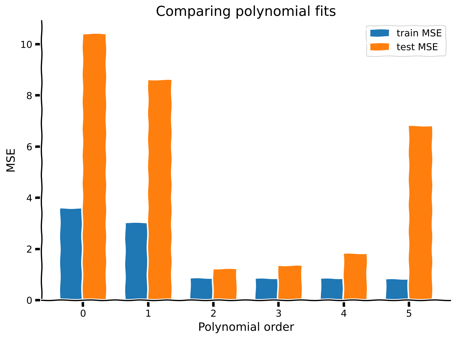
plot_MSE_poly_fits(mse_train, mse_test, max_order)

解答を見る$

出力例:

# @title Submit your feedback
content_review(f"{feedback_prefix}_Compute_train_vs_test_error_Exercise")

上のプロットからわかるように、より複雑なモデル（高次多項式）は訓練データに対するMSEが低くなります。過度に単純化されたモデル（次数0と1）は訓練データに対してMSEが高いです。モデルの複雑さを増すにつれて、バイアスが高い状態から低い状態へと変化します。

テストデータに対するMSEは異なるパターンを示します。最良のテストMSEは次数2のモデルで、これはデータが次数2のモデルで生成されたため理にかなっています。より単純なモデルもより複雑なモデルもテストMSEは高くなります。

まとめると:

次数0モデル: 高バイアス、低バリアンス

次数5モデル: 低バイアス、高バリアンス

次数2モデル: ちょうど良い、低バイアス、低バリアンス

まとめ

推定所要時間: 25分

訓練データはフィッティングに使うデータ、テストデータは保持されたデータです。
バイアスとバリアンスの適切なバランスを取る必要があります。理想的にはバイアスもバリアンスも低い最適なモデル複雑さを持つモデルを見つけたいです。
複雑すぎるモデルはバイアスが低くバリアンスが高いです。
単純すぎるモデルはバイアスが高くバリアンスが低いです。

注意

バイアスとバリアンスは現代の機械学習で非常に重要な概念ですが、最近では必ずしもトレードオフしないことが観察されています（例えば「ダブルディセント」の現象と理論を参照してください）

さらなる参考文献:

Hastie, Tibshirani, Friedman著『The Elements of Statistical Learning』(https://web.stanford.edu/~hastie/ElemStatLearn/)

ボーナス

ボーナス演習: バイアス・バリアンス分解の証明

MSEのバイアス・バリアンス分解を証明してください。

\mathbb{E}_{x}\left[\left(y-\hat{y}(x ; \theta)\right)^{2}\right]=\left(\operatorname{Bias}_{x}[\hat{y}(x ; \theta)]\right)^{2}+\operatorname{Var}_{x}[\hat{y}(x ; \theta)]+\sigma^{2}

ここで

\operatorname{Bias}_{x}[\hat{y}(x ; \theta)]=\mathbb{E}_{x}[\hat{y}(x ; \theta)]-y

および

\operatorname{Var}_{x}[\hat{y}(x ; \theta)]=\mathbb{E}_{x}\left[\hat{y}(x ; \theta)^{2}\right]-\mathrm{E}_{x}[\hat{y}(x ; \theta)]^{2}

ヒントはこちらをクリック

次の式を使ってください:

\operatorname{Var}[X]=\mathbb{E}\left[X^{2}\right]-(\mathrm{E}[X])^{2}

# @title Submit your feedback
content_review(f"{feedback_prefix}_Proof_bias_variance_for_MSE_Bonus_Exercise")