チュートリアル 4: 重回帰分析と多項式回帰

第1週、第2日目: モデルフィッティング

Neuromatch Academyによる

コンテンツ作成者: Pierre-Étienne Fiquet, Anqi Wu, Alex Hyafil（Byron Galbraith, Ella Battyの協力を得て）

コンテンツレビュアー: Lina Teichmann, Saeed Salehi, Patrick Mineault, Michael Waskom

制作編集者: Spiros Chavlis

チュートリアルの目的

チュートリアルの推定所要時間: 35分

これはデータにモデルをフィットさせるシリーズのチュートリアル4です。まずは単純な線形回帰を、最小二乗法（チュートリアル1）と最尤推定（チュートリアル2）を使って学びました。推定された線形モデルのパラメータの信頼区間をブートストラップで構築する方法も学びました（チュートリアル3）。今回のチュートリアル4では、重回帰分析と多項式回帰に一般化して回帰モデルの探求を終えます。最後に、これらのモデルの中からどのモデルを選ぶかを学びます。バイアス・バリアンストレードオフ（チュートリアル5）とモデル選択のためのクロスバリデーション（チュートリアル6）についても議論します。

本チュートリアルでは、複数の特徴量を取り入れた回帰モデルに一般化します。

『デザインマトリックス』を使った回帰の入力構造の学習
複数特徴量に対するMSEの一般化と最小二乗推定量の利用
多次元でのデータとモデルフィットの可視化
複雑さの異なる多項式回帰モデルのフィッティング
多項式回帰のフィット結果のプロットと評価

# @title Tutorial slides
# @markdown These are the slides for the videos in all tutorials today
from IPython.display import IFrame
link_id = "2mkq4"
print(f"If you want to download the slides: https://osf.io/download/{link_id}/")
IFrame(src=f"https://mfr.ca-1.osf.io/render?url=https://osf.io/{link_id}/?direct%26mode=render%26action=download%26mode=render", width=854, height=480)

セットアップ

# @title Install and import feedback gadget


from vibecheck import DatatopsContentReviewContainer
def content_review(notebook_section: str):
    return DatatopsContentReviewContainer(
        "",  # No text prompt
        notebook_section,
        {
            "url": "https://pmyvdlilci.execute-api.us-east-1.amazonaws.com/klab",
            "name": "neuromatch_cn",
            "user_key": "y1x3mpx5",
        },
    ).render()


feedback_prefix = "W1D2_T4"

# Imports
import numpy as np
import matplotlib.pyplot as plt

# @title Figure Settings
import logging
logging.getLogger('matplotlib.font_manager').disabled = True

%config InlineBackend.figure_format = 'retina'
plt.style.use("https://raw.githubusercontent.com/NeuromatchAcademy/course-content/main/nma.mplstyle")

# @title Plotting Functions

def evaluate_fits(order_list, mse_list):
  """ Compare the quality of multiple polynomial fits
  by plotting their MSE values.

  Args:
    order_list (list): list of the order of polynomials to be compared
    mse_list (list): list of the MSE values for the corresponding polynomial fit
  """
  fig, ax = plt.subplots()
  ax.bar(order_list, mse_list)
  ax.set(title='Comparing Polynomial Fits', xlabel='Polynomial order', ylabel='MSE')
  plt.show()


def plot_fitted_polynomials(x, y, theta_hat):
  """ Plot polynomials of different orders

  Args:
    x (ndarray): input vector of shape (n_samples)
    y (ndarray): vector of measurements of shape (n_samples)
    theta_hat (dict): polynomial regression weights for different orders
  """

  x_grid = np.linspace(x.min() - .5, x.max() + .5)

  plt.figure()

  for order in range(0, max_order + 1):
    X_design = make_design_matrix(x_grid, order)
    plt.plot(x_grid, X_design @ theta_hat[order]);

  plt.ylabel('y')
  plt.xlabel('x')
  plt.plot(x, y, 'C0.');
  plt.legend([f'order {o}' for o in range(max_order + 1)], loc=1)
  plt.title('polynomial fits')
  plt.show()

セクション1: 重回帰分析

チュートリアル開始からここまでの推定所要時間: 8分

この動画では、複数入力（1次元以上）の線形回帰と多項式回帰について扱います。

動画のテキスト要約はこちらをクリック

単変量の場合と推定量の信頼区間の作り方を考えたので、次は一般的な線形回帰の場合に移ります。ここでは入力に複数の回帰子（特徴量）が含まれます。

元の単変量線形モデルは次のように表されました。

y = \theta x + \epsilon

ここで $\theta$ は傾き、 $\epsilon$ はノイズです。これを多変量に拡張すると、特徴量ごとにパラメータを追加します。

y = \theta_0 + \theta_1 x_1 + \theta_2 x_2 + ... +\theta_d x_d + \epsilon

ここで $\theta_0$ は切片、 $d$ は特徴量の数（入力の次元数）です。

1つのデータ点についてはベクトル表記で簡潔に書けます。

y_i = \boldsymbol{\theta}^{\top}\mathbf{x}_i + \epsilon

行列形式では

\mathbf{y} = \mathbf{X}\boldsymbol{\theta} + \mathbf{\epsilon}

ここで $\mathbf{y}$ は測定値のベクトル、 $\mathbf{X}$ は各入力サンプル（行）ごとの特徴量値（列）を含む行列、 $\boldsymbol{\theta}$ はパラメータベクトルです。

この行列 $\mathbf{X}$ はしばしば「デザインマトリックス$」と呼ばれます。

最適なパラメータベクトル $\boldsymbol{\hat\theta}$ を求めたいです。単一回帰子のMSE最小化の解析解は

\hat\theta = \frac{\sum_{i=1}^N x_i y_i}{\sum_{i=1}^N x_i^2}.

多回帰子の場合も同様で、行列形式で表すと

\boldsymbol{\hat\theta} = (\mathbf{X}^\top\mathbf{X})^{-1}\mathbf{X}^\top\mathbf{y}.

これは最小二乗法$ (OLS)推定量と呼ばれます。

# @title Video 1: Multiple Linear Regression and Polynomial Regression
from ipywidgets import widgets
from IPython.display import YouTubeVideo
from IPython.display import IFrame
from IPython.display import display


class PlayVideo(IFrame):
  def __init__(self, id, source, page=1, width=400, height=300, **kwargs):
    self.id = id
    if source == 'Bilibili':
      src = f'https://player.bilibili.com/player.html?bvid={id}&page={page}'
    elif source == 'Osf':
      src = f'https://mfr.ca-1.osf.io/render?url=https://osf.io/download/{id}/?direct%26mode=render'
    super(PlayVideo, self).__init__(src, width, height, **kwargs)


def display_videos(video_ids, W=400, H=300, fs=1):
  tab_contents = []
  for i, video_id in enumerate(video_ids):
    out = widgets.Output()
    with out:
      if video_ids[i][0] == 'Youtube':
        video = YouTubeVideo(id=video_ids[i][1], width=W,
                             height=H, fs=fs, rel=0)
        print(f'Video available at https://youtube.com/watch?v={video.id}')
      else:
        video = PlayVideo(id=video_ids[i][1], source=video_ids[i][0], width=W,
                          height=H, fs=fs, autoplay=False)
        if video_ids[i][0] == 'Bilibili':
          print(f'Video available at https://www.bilibili.com/video/{video.id}')
        elif video_ids[i][0] == 'Osf':
          print(f'Video available at https://osf.io/{video.id}')
      display(video)
    tab_contents.append(out)
  return tab_contents


video_ids = [('Youtube', 'd4nfTki6Ejc'), ('Bilibili', 'BV11Z4y1u7cf')]
tab_contents = display_videos(video_ids, W=854, H=480)
tabs = widgets.Tab()
tabs.children = tab_contents
for i in range(len(tab_contents)):
  tabs.set_title(i, video_ids[i][0])
display(tabs)

# @title Submit your feedback
content_review(f"{feedback_prefix}_Multiple_Linear_Regression_and_Polynomial_Regression_Video")

このチュートリアルでは、2次元の場合（ $d=2$ ）に焦点を当てます。これにより結果を簡単に可視化できます。例えば、科学者が網膜神経節細胞のスパイク応答を、コントラストと方向の異なる光刺激パターンに対して記録したとします。この場合、コントラストと方向の値を特徴量／回帰子として細胞の応答を予測できます。

この場合、単一データ点のモデルは次のように書けます。

y = \theta_0 + \theta_1 x_1 + \theta_2 x_2 + \epsilon

複数データ点の場合は行列形式で、

\mathbf{X} = \begin{bmatrix} 1 & x_{1,1} & x_{1,2} \\ 1 & x_{2,1} & x_{2,2} \\ \vdots & \vdots & \vdots \\ 1 & x_{n,1} & x_{n,2} \end{bmatrix}, \boldsymbol{\theta} = \begin{bmatrix} \theta_0 \\ \theta_1 \\ \theta_2 \\ \end{bmatrix}

ここで $x_{i,j}$ はi番目のデータ点のj番目の特徴量を意味します。

実際の探索用データセットでは $\boldsymbol{\theta}=[0, -2, -3]$ と設定し、 $x \in [-2,2)$ から $N=40$ のノイズを含むサンプルを生成します。 $\theta_0=0$ に設定するとオフセット項は無視されます。

# @markdown Execute this cell to simulate some data

# Set random seed for reproducibility
np.random.seed(1234)

# Set parameters
theta = [0, -2, -3]
n_samples = 40

# Draw x and calculate y
n_regressors = len(theta)
x0 = np.ones((n_samples, 1))
x1 = np.random.uniform(-2, 2, (n_samples, 1))
x2 = np.random.uniform(-2, 2, (n_samples, 1))
X = np.hstack((x0, x1, x2))
noise = np.random.randn(n_samples)
y = X @ theta + noise


ax = plt.subplot(projection='3d')
ax.plot(X[:,1], X[:,2], y, '.')

ax.set(
    xlabel='$x_1$',
    ylabel='$x_2$',
    zlabel='y'
)
plt.tight_layout()

コーディング演習1: 最小二乗推定量

この演習では、デザインマトリックス $\mathbf{X}$ と測定ベクトル $\mathbf{y}$ から $\boldsymbol{\hat\theta}$ をOLSで推定する関数を実装します。行列積には@、転置は.T、行列の逆行列はnp.linalg.invを使えます。

def ordinary_least_squares(X, y):
  """Ordinary least squares estimator for linear regression.

  Args:
    x (ndarray): design matrix of shape (n_samples, n_regressors)
    y (ndarray): vector of measurements of shape (n_samples)

  Returns:
    ndarray: estimated parameter values of shape (n_regressors)
  """
  ######################################################################
  ## TODO for students: solve for the optimal parameter vector using OLS
  # Fill out function and remove
  raise NotImplementedError("Student exercise: solve for theta_hat vector using OLS")
  ######################################################################

  # Compute theta_hat using OLS
  theta_hat = ...

  return theta_hat


theta_hat = ordinary_least_squares(X, y)
print(theta_hat)

この関数を完成させると、$\boldsymbol{\hat\theta} = $
[ 0.13861386, -2.09395731, -3.16370742]
となるはずです。

解答を見る$

# @title Submit your feedback
content_review(f"{feedback_prefix}_Ordinary_Least_Squares_Estimator_Exercise")

$\boldsymbol{\hat\theta}$ が得られたので、 $\hat{\mathbf{y}}$ を計算し、平均二乗誤差（MSE）を求められます。

# Compute predicted data
theta_hat = ordinary_least_squares(X, y)
y_hat = X @ theta_hat

# Compute MSE
print(f"MSE = {np.mean((y - y_hat)**2):.2f}")

最後に、以下のコードはデータ点（青）とフィットした平面の幾何学的な可視化を行います。

# @markdown Execute this cell to visualize data and predicted plane

theta_hat = ordinary_least_squares(X, y)
xx, yy = np.mgrid[-2:2:50j, -2:2:50j]
y_hat_grid = np.array([xx.flatten(), yy.flatten()]).T @ theta_hat[1:]
y_hat_grid = y_hat_grid.reshape((50, 50))

ax = plt.subplot(projection='3d')
ax.plot(X[:, 1], X[:, 2], y, '.')
ax.plot_surface(xx, yy, y_hat_grid, linewidth=0, alpha=0.5, color='C1',
                cmap=plt.get_cmap('coolwarm'))

for i in range(len(X)):
  ax.plot((X[i, 1], X[i, 1]),
          (X[i, 2], X[i, 2]),
          (y[i], y_hat[i]),
          'g-', alpha=.5)

ax.set(
    xlabel='$x_1$',
    ylabel='$x_2$',
    zlabel='y'
)
plt.tight_layout()
plt.show()

セクション2: 多項式回帰

これまでに、線形回帰モデルを使って入力から出力を予測する方法を学びました。これにより神経科学を含む様々な関係性をモデル化できます。

この方法の潜在的な問題はモデルの単純さです。線形回帰は名前の通り、入力と出力の間の線形関係しか捉えられません。言い換えれば、予測出力は入力の重み付き和に過ぎません。もしもっと複雑な計算が起きていたら？幸い、多くのより複雑なモデルが存在し（今後3週間で多く出会います）、その中でも理解しやすくフィットも簡単なモデルの一つが多項式回帰です。これは線形回帰の拡張です。

動画の関連部分のテキスト要約はこちらをクリック

多項式回帰は線形回帰の拡張なので、これまで学んだことが役立ちます！目的は同じで、入力 $x$ から従属変数 $y$ を予測します。違いはモデルが捉える入力と出力の関係の種類です。

線形回帰モデルは入力の重み付き和で出力を予測します。

y = \theta_0 + \theta x + \epsilon

多項式回帰では、入力に基づく多項式方程式として出力をモデル化します。例えば、

y = \theta_0 + \theta_1 x + \theta_2 x^2 + \theta_3 x^3 + \epsilon

多項式の次数を変えることで複雑さを調整できます。次数は多項式の最高べき乗を指します。上の式は3次多項式です。さらに項を追加して4次多項式（ $+ \theta_4 x^4$ ）なども可能です。

まず、データをシミュレートして多項式回帰モデルのフィッティングを練習します。ランダムな入力 $x$ を生成し、 $y = x^2 - x - 2$ に従い、入力と出力にノイズを加えて実際の状況に近づけます。

# @markdown Execute this cell to simulate some data

# setting a fixed seed to our random number generator ensures we will always
# get the same psuedorandom number sequence
np.random.seed(121)
n_samples = 30
x = np.random.uniform(-2, 2.5, n_samples)  # inputs uniformly sampled from [-2, 2.5)
y =  x**2 - x - 2   # computing the outputs

output_noise = 1/8 * np.random.randn(n_samples)
y += output_noise  # adding some output noise

input_noise = 1/2 * np.random.randn(n_samples)
x += input_noise  # adding some input noise

fig, ax = plt.subplots()
ax.scatter(x, y)  # produces a scatter plot
ax.set(xlabel='x', ylabel='y');

セクション2.1: 多項式回帰のデザインマトリックス

チュートリアル開始からここまでの推定所要時間: 16分

多項式回帰の基本的な考え方とノイズのあるデータが得られたので始めましょう！線形回帰モデルと多項式回帰モデルの違いは入力変数の構造にあります。

1つの特徴量の場合に戻ります。線形回帰では $\mathbf{X} = \mathbf{x}$ を入力データとして使いました。ここで $\mathbf{x}$ は各要素が1つのデータ点の入力値のベクトルです。定数バイアス（2次元プロットのy切片）を加えるために $\mathbf{X} = \big[ \boldsymbol 1, \mathbf{x} \big]$ とし、 $\boldsymbol 1$ は全て1の列ベクトルです。フィッティング時にはこの行列の各列に重みを学習します。つまり、1列目は全て1なのでバイアスパラメータ（ $+ \theta_0$ ）を学習します。

この入力に使う行列 $\mathbf{X}$ はデザインマトリックスと呼ばれます。 $\mathbf{x}^2, \mathbf{x}^3$ などの重みも学習したいので、多項式回帰の次数 $k$ に対してデザインマトリックスは次のように構築します。

\mathbf{X} = \big[ \boldsymbol 1 , \mathbf{x}^1, \mathbf{x}^2 , \ldots , \mathbf{x}^k \big],

ここで $\boldsymbol{1}$ は $\mathbf{x}$ と同じ長さの全て1のベクトル、 $\mathbf{x}^p$ は $\mathbf{x}$ の各要素を $p$ 乗したベクトルです。なお $\boldsymbol{1} = \mathbf{x}^0$ 、 $\mathbf{x}^1 = \mathbf{x}$ です。

複数特徴量がある場合は、同様に各特徴量を各べき乗に上げて含めます。例えば、2つの特徴量があるとき、 $\mathbf{x}_m$ が1つ目の特徴量のベクトル、 $\mathbf{x}_n$ が2つ目の特徴量のベクトルなら、デザインマトリックスは

\mathbf{X} = \big[ \boldsymbol 1 , \mathbf{x}_m^1, \mathbf{x}_n^1, \mathbf{x}_m^2 , \mathbf{x}_n^2\ldots , \mathbf{x}_m^k , \mathbf{x}_n^k \big],

コーディング演習2.1: デザインマトリックスの構築

入力データとフィットしたい多項式の次数を受け取り、デザインマトリックスを構築する関数(make_design_matrix)を作成してください。データと次数5のときのデザインマトリックスの一部を表示します。

def make_design_matrix(x, order):
  """Create the design matrix of inputs for use in polynomial regression

  Args:
    x (ndarray): input vector of shape (n_samples)
    order (scalar): polynomial regression order

  Returns:
    ndarray: design matrix for polynomial regression of shape (samples, order+1)
  """
  ########################################################################
  ## TODO for students: create the design matrix ##
  # Fill out function and remove
  raise NotImplementedError("Student exercise: create the design matrix")
  ########################################################################

  # Broadcast to shape (n x 1) so dimensions work
  if x.ndim == 1:
    x = x[:, None]

  #if x has more than one feature, we don't want multiple columns of ones so we assign
  # x^0 here
  design_matrix = np.ones((x.shape[0], 1))

  # Loop through rest of degrees and stack columns (hint: np.hstack)
  for degree in range(1, order + 1):
      design_matrix = ...

  return design_matrix


order = 5
X_design = make_design_matrix(x, order)

print(X_design[0:2, 0:2])

表示されるデザインマトリックスの一部は

[[ 1.         -1.51194917]
 [ 1.         -0.35259945]]

解答を見る$

セクション2.2: 多項式回帰モデルのフィッティング

チュートリアル開始からここまでの推定所要時間: 24分

入力が正しくデザインマトリックスに構造化できたので、多項式回帰のフィッティングは線形回帰モデルのフィッティングと同じです！必要な多項式の構造は入力のデザインマトリックスの構造に含まれているため、これまでの最小二乗解を使えます。

コーディング演習2.2: 異なる次数の多項式回帰モデルのフィッティング

ここでは、多項式の次数を変えながら回帰係数（ $\theta_0, \theta_1, \theta_2, \ldots$ ）を求める関数solve_poly_regを作成します。max_orderまでの次数をループし、それぞれのモデルをフィットして重みを保存します。ordinary_least_squares関数を呼び出しても構いません。

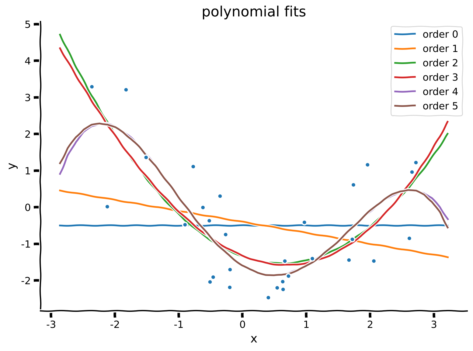
その後、データの上にフィットした多項式をプロットしてフィットの質を定性的に確認します。滑らかな曲線を見るために、データセットの入力の最大値と最小値の範囲でグリッド上に評価します。

def solve_poly_reg(x, y, max_order):
  """Fit a polynomial regression model for each order 0 through max_order.

  Args:
    x (ndarray): input vector of shape (n_samples)
    y (ndarray): vector of measurements of shape (n_samples)
    max_order (scalar): max order for polynomial fits

  Returns:
    dict: fitted weights for each polynomial model (dict key is order)
  """

  # Create a dictionary with polynomial order as keys,
  # and np array of theta_hat (weights) as the values
  theta_hats = {}

  # Loop over polynomial orders from 0 through max_order
  for order in range(max_order + 1):

    ##################################################################################
    ## TODO for students: Create design matrix and fit polynomial model for this order
    # Fill out function and remove
    raise NotImplementedError("Student exercise: fit a polynomial model")
    ##################################################################################

    # Create design matrix
    X_design = ...

    # Fit polynomial model
    this_theta = ...

    theta_hats[order] = this_theta

  return theta_hats


max_order = 5
theta_hats = solve_poly_reg(x, y, max_order)

# Visualize
plot_fitted_polynomials(x, y, theta_hats)

解答を見る$

例の出力:

セクション2.3: フィットの質の評価

チュートリアル開始からここまでの推定所要時間: 29分

線形回帰と同様に、平均二乗誤差（MSE）を計算してモデルのフィットの良さを評価できます。

MSEは次のように計算します。

\mathrm{MSE} = \frac 1 N ||\mathbf{y} - \hat{\mathbf{y}}||^2 = \frac 1 N \sum_{i=1}^N (y_i - \hat y_i)^2

ここで各モデルの予測値は$ \hat{\mathbf{y}} = \mathbf{X}\boldsymbol{\hat\theta}$です。

どのモデル（多項式の次数）が最も良いMSEになると思いますか？

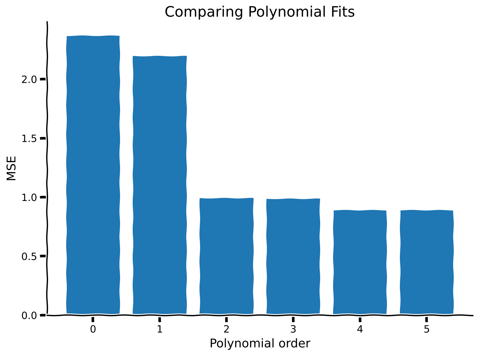
コーディング演習2.3: MSEの計算とモデル比較

異なる多項式次数のMSEを計算し、棒グラフで比較します。

mse_list = []
order_list = list(range(max_order + 1))

for order in order_list:

  X_design = make_design_matrix(x, order)

  ########################################################################
  ## TODO for students
  # Fill out function and remove
  raise NotImplementedError("Student exercise: compute MSE")
  ########################################################################

  # Get prediction for the polynomial regression model of this order
  y_hat = ...

  # Compute the residuals
  residuals = ...

  # Compute the MSE
  mse = ...

  mse_list.append(mse)


# Visualize MSE of fits
evaluate_fits(order_list, mse_list)

解答を見る$

例の出力:

まとめ

チュートリアルの推定所要時間: 35分

線形回帰は自然に多次元に一般化できる
線形代数は2次元を超えた問題を数学的に扱い解くための強力なツールを提供する
線形回帰モデルから多項式回帰モデルに変えるには、入力データの構造を変えるだけでよい
多項式モデルの次数を変えることでモデルの複雑さを選べる
高次の多項式モデルはフィットしたデータに対してMSEが低くなる傾向がある

注意: 実際には、多次元の最小二乗問題はLAPACKなどの数値計算ルーチンのおかげで非常に効率的に解ける。

記法

\begin{align}
x & $\quad \text{入力、独立変数}$ \
y & $\quad \text{応答測定値、従属変数}$ \
$\epsilon$ & $\quad \text{測定誤差、ノイズ成分}$ \
$\theta$ & $\quad \text{傾きパラメータ}$ \
$\hat{\theta}$ & $\quad \text{推定された傾きパラメータ}$ \
$\mathbf{x}$ & $\quad \text{各要素が異なるデータ点の入力ベクトル}$ \
$\mathbf{X}$ & $\quad \text{デザインマトリックス}$ \
$\mathbf{y}$ & $\quad \text{測定値のベクトル}$ \
$\mathbf{\hat y}$ & $\quad \text{推定された測定値のベクトル}$ \
$\boldsymbol{\theta}$ & $\quad \text{パラメータのベクトル}$ \
$\boldsymbol{\hat\theta}$ & $\quad \text{推定されたパラメータのベクトル}$ \
d & $\quad \text{入力の次元数}$ \
N & $\quad \text{サンプル数}$ \
\end{align}

推奨文献

Introduction to Applied Linear Algebra – Vectors, Matrices, and Least Squares by Stephen Boyd and Lieven Vandenberghe