チュートリアル 3: 信頼区間とブートストラップ

第1週、第2日目: モデルフィッティング

Neuromatch Academyによる

コンテンツ作成者: Pierre-Étienne Fiquet, Anqi Wu, Alex Hyafil（Byron Galbraithの協力を得て）

コンテンツレビュアー: Lina Teichmann, Saeed Salehi, Patrick Mineault, Ella Batty, Michael Waskom

制作編集者: Spiros Chavlis

チュートリアルの目的

チュートリアルの推定所要時間: 23分

これはデータにモデルをフィットさせるシリーズのチュートリアル3です。最初に単純な線形回帰を、最小二乗法（チュートリアル1）と最尤推定（チュートリアル2）を使って行いました。今回はブートストラップを用いて推定した線形モデルのパラメータの信頼区間を構築します（チュートリアル3）。回帰モデルの探求は多変量線形回帰や多項式回帰への一般化（チュートリアル4）で終わります。最後にこれらのモデルの選択方法を学びます。バイアス・バリアンスのトレードオフ（チュートリアル5）やモデル選択のためのクロスバリデーション（チュートリアル6）について議論します。

このチュートリアルでは、推定したモデルパラメータの良さを評価する方法について説明します。

• ブートストラップを使って新しいサンプルデータセットを生成する方法を学ぶ
• これらの新しいサンプルデータセットでモデルパラメータを推定する
• 信頼区間を使って推定値の分散を定量化する

# @title Tutorial slides
# @markdown These are the slides for the videos in all tutorials today
from IPython.display import IFrame
link_id = "2mkq4"
print(f"If you want to download the slides: https://osf.io/download/{link_id}/")
IFrame(src=f"https://mfr.ca-1.osf.io/render?url=https://osf.io/{link_id}/?direct%26mode=render%26action=download%26mode=render", width=854, height=480)

セットアップ

# @title Install and import feedback gadget


from vibecheck import DatatopsContentReviewContainer
def content_review(notebook_section: str):
    return DatatopsContentReviewContainer(
        "",  # No text prompt
        notebook_section,
        {
            "url": "https://pmyvdlilci.execute-api.us-east-1.amazonaws.com/klab",
            "name": "neuromatch_cn",
            "user_key": "y1x3mpx5",
        },
    ).render()


feedback_prefix = "W1D2_T3"

# Imports
import numpy as np
import matplotlib.pyplot as plt

# @title Figure Settings
import logging
logging.getLogger('matplotlib.font_manager').disabled = True

%config InlineBackend.figure_format = 'retina'
plt.style.use("https://raw.githubusercontent.com/NeuromatchAcademy/course-content/main/nma.mplstyle")

# @title Plotting Functions

def plot_original_and_resample(x, y, x_, y_):
  """ Plot the original sample and the resampled points from this sample.

  Args:
    x (ndarray): An array of shape (samples,) that contains the input values.
    y (ndarray): An array of shape (samples,) that contains the corresponding
      measurement values to the inputs.
    x_ (ndarray): An array of shape (samples,) with a subset of input values from x
    y_ (ndarray): An array of shape (samples,) with a the corresponding subset
      of measurement values as x_ from y

  """
  fig, (ax1, ax2) = plt.subplots(ncols=2, figsize=(12, 5))
  ax1.scatter(x, y)
  ax1.set(title='Original', xlabel='x', ylabel='y')

  ax2.scatter(x_, y_, color='c')

  ax2.set(title='Resampled', xlabel='x', ylabel='y',
          xlim=ax1.get_xlim(), ylim=ax1.get_ylim())
  plt.show()

はじめに

これまで観測データにフィットするモデルパラメータを推定する方法を探ってきました。アプローチは、平均二乗誤差を最小化するか、尤度を最大化するかのいずれかの基準を最適化し、全データセットを使うものでした。推定値は本当にどれくらい良いのでしょうか？まだ見ていない新しいデータを記述するのにどれほど自信を持てるでしょうか？

一つの解決策は単により多くのデータを収集し、以前推定したパラメータでこの新しいデータセットのMSEをチェックすることです。しかしこれは常に可能とは限らず、モデルの精度にどれほど定量的に自信があるかという問題は残ります。

セクション1ではブートストラップの実装方法を探ります。セクション2ではブートストラップ法を使って推定値の信頼区間を構築します。

# @title Video 1: Confidence Intervals & Bootstrapping
from ipywidgets import widgets
from IPython.display import YouTubeVideo
from IPython.display import IFrame
from IPython.display import display


class PlayVideo(IFrame):
  def __init__(self, id, source, page=1, width=400, height=300, **kwargs):
    self.id = id
    if source == 'Bilibili':
      src = f'https://player.bilibili.com/player.html?bvid={id}&page={page}'
    elif source == 'Osf':
      src = f'https://mfr.ca-1.osf.io/render?url=https://osf.io/download/{id}/?direct%26mode=render'
    super(PlayVideo, self).__init__(src, width, height, **kwargs)


def display_videos(video_ids, W=400, H=300, fs=1):
  tab_contents = []
  for i, video_id in enumerate(video_ids):
    out = widgets.Output()
    with out:
      if video_ids[i][0] == 'Youtube':
        video = YouTubeVideo(id=video_ids[i][1], width=W,
                             height=H, fs=fs, rel=0)
        print(f'Video available at https://youtube.com/watch?v={video.id}')
      else:
        video = PlayVideo(id=video_ids[i][1], source=video_ids[i][0], width=W,
                          height=H, fs=fs, autoplay=False)
        if video_ids[i][0] == 'Bilibili':
          print(f'Video available at https://www.bilibili.com/video/{video.id}')
        elif video_ids[i][0] == 'Osf':
          print(f'Video available at https://osf.io/{video.id}')
      display(video)
    tab_contents.append(out)
  return tab_contents


video_ids = [('Youtube', 'hs6bVGQNSIs'), ('Bilibili', 'BV1vK4y1s7py')]
tab_contents = display_videos(video_ids, W=854, H=480)
tabs = widgets.Tab()
tabs.children = tab_contents
for i in range(len(tab_contents)):
  tabs.set_title(i, video_ids[i][0])
display(tabs)

# @title Submit your feedback
content_review(f"{feedback_prefix}_Confidence_Intervals_and_Bootstrapping_Video")

セクション1: ブートストラップ

チュートリアル開始からここまでの推定所要時間: 7分

ブートストラップは推定パラメータの信頼性や不確実性を評価するための広く使われる方法で、元々はBradley Efron$によって提案されました。アイデアは、元の真のデータセットからランダムにサンプリングして多くの新しい合成データセットを生成し、それぞれのデータセットで推定量を求め、最後にこれらすべての推定量の分布を見て信頼度を定量化することです。

新しくリサンプリングされた各データセットは元のサイズと同じで、データ点は復元抽出（重複を許す）でサンプリングされます。つまり同じデータ点が複数回現れることがあります。実際には多くのリサンプリングデータセットが必要で、ここでは2000個を使います。

この考えを探るために、ノイズのあるサンプルを線形モデル $y_i = 1.2x_i + \epsilon_i$ に沿って再び使いますが、今回は前回の半分のデータ点（30点の代わりに15点）だけを使います。

#@title

#@markdown Execute this cell to simulate some data

# setting a fixed seed to our random number generator ensures we will always
# get the same psuedorandom number sequence
np.random.seed(121)

# Let's set some parameters
theta = 1.2
n_samples = 15

# Draw x and then calculate y
x = 10 * np.random.rand(n_samples)  # sample from a uniform distribution over [0,10)
noise = np.random.randn(n_samples)  # sample from a standard normal distribution
y = theta * x + noise

fig, ax = plt.subplots()
ax.scatter(x, y)  # produces a scatter plot
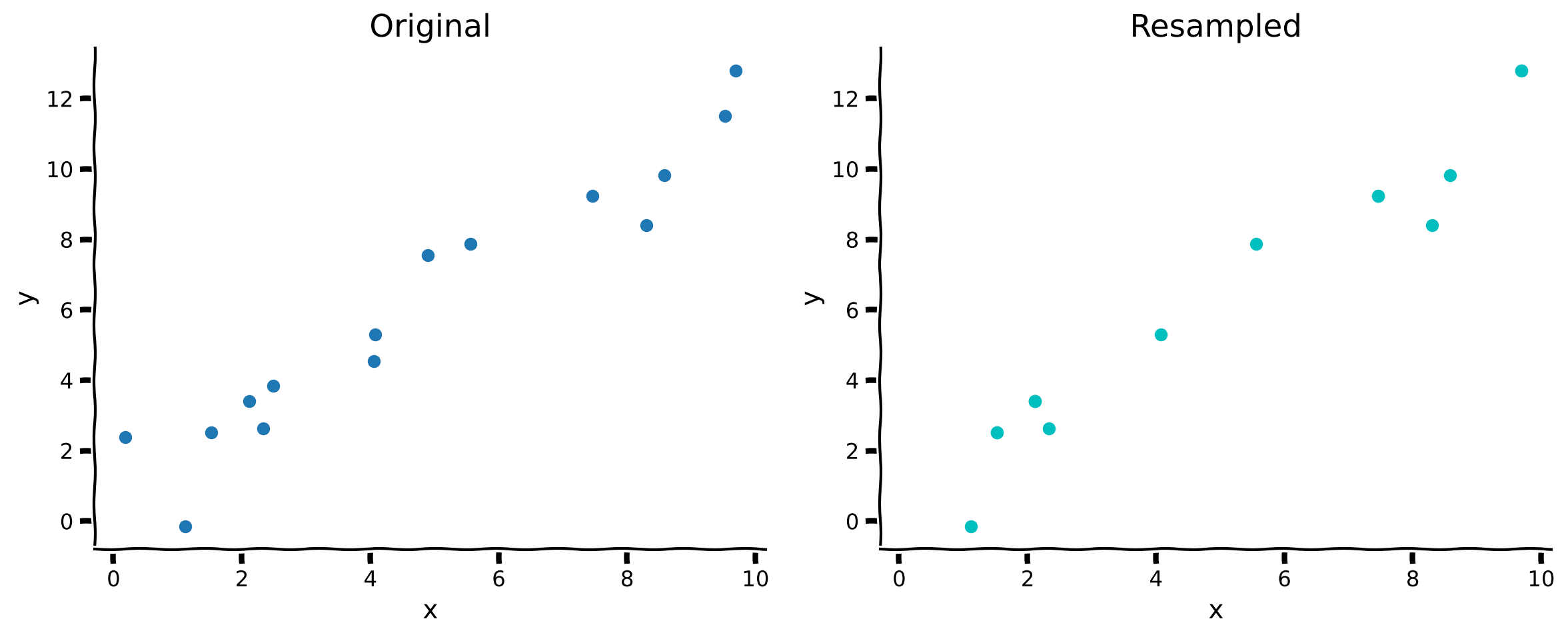
ax.set(xlabel='x', ylabel='y');

コーディング演習1: 復元抽出によるデータセットのリサンプリング

この演習では、復元抽出でデータセットをリサンプリングするメソッドを実装します。このメソッドは $\mathbf{x}$ と $\mathbf{y}$ の配列を受け取り、元の配列からランダムにサンプリングして作成した新しい $\mathbf{x}'$ と $\mathbf{y}'$ の配列を返すべきです。

その後、元のデータセットとリサンプリングしたデータセットを比較します。

ヒント: numpy.random.choice メソッドが役立ちます。

def resample_with_replacement(x, y):
  """Resample data points with replacement from the dataset of `x` inputs and
  `y` measurements.

  Args:
    x (ndarray): An array of shape (samples,) that contains the input values.
    y (ndarray): An array of shape (samples,) that contains the corresponding
      measurement values to the inputs.

  Returns:
    ndarray, ndarray: The newly resampled `x` and `y` data points.
  """
  #######################################################
  ## TODO for students: resample dataset with replacement
  # Fill out function and remove
  raise NotImplementedError("Student exercise: resample dataset with replacement")
  #######################################################

  # Get array of indices for resampled points
  sample_idx = ...

  # Sample from x and y according to sample_idx
  x_ = ...
  y_ = ...

  return x_, y_

x_, y_ = resample_with_replacement(x, y)

plot_original_and_resample(x, y, x_, y_)

解答を見る$

出力例:

# @title Submit your feedback
content_review(f"{feedback_prefix}_Resample_dataset_with_replacement_Exercise")

右側のリサンプリングされたプロットでは、実際の点の数は同じですが、一部の点が繰り返されているため一度しか表示されていません。

これでデータをリサンプリングする方法ができたので、これを使ってブートストラップの全過程を実行できます。

コーディング演習2: ブートストラップ推定

この演習では、入力 ($\mathbf{x}$) と測定値 ($\mathbf{y}$) のデータセットから一連の $\hat\theta$ 値を生成するブートストラップ処理を実装します。ここでは resample_with_replacement を使い、チュートリアル1のヘルパー関数 solve_normal_eqn を呼び出してMSEに基づく推定量を算出してもよいです。

この関数を使って異なるサンプルからの $\hat{\theta}$ を見てみましょう。

# @markdown Execute this cell for helper function `solve_normal_eqn`
def solve_normal_eqn(x, y):
  """Solve the normal equations to produce the value of theta_hat that minimizes
    MSE.

    Args:
    x (ndarray): An array of shape (samples,) that contains the input values.
    y (ndarray): An array of shape (samples,) that contains the corresponding
      measurement values to the inputs.
    thata_hat (float): An estimate of the slope parameter.

  Returns:
    float: the value for theta_hat arrived from minimizing MSE
  """
  theta_hat = (x.T @ y) / (x.T @ x)
  return theta_hat

def bootstrap_estimates(x, y, n=2000):
  """Generate a set of theta_hat estimates using the bootstrap method.

  Args:
    x (ndarray): An array of shape (samples,) that contains the input values.
    y (ndarray): An array of shape (samples,) that contains the corresponding
      measurement values to the inputs.
    n (int): The number of estimates to compute

  Returns:
    ndarray: An array of estimated parameters with size (n,)
  """
  theta_hats = np.zeros(n)

  ##############################################################################
  ## TODO for students: implement bootstrap estimation
  # Fill out function and remove
  raise NotImplementedError("Student exercise: implement bootstrap estimation")
  ##############################################################################

  # Loop over number of estimates
  for i in range(n):

    # Resample x and y
    x_, y_ = ...

    # Compute theta_hat for this sample
    theta_hats[i] = ...

  return theta_hats


# Set random seed
np.random.seed(123)

# Get bootstrap estimates
theta_hats = bootstrap_estimates(x, y, n=2000)
print(theta_hats[0:5])

最初の5つの推定値は [1.27550888 1.17317819 1.18198819 1.25329255 1.20714664] になるはずです。

解答を見る$

# @title Submit your feedback
content_review(f"{feedback_prefix}_Bootsrap_Estimates_Exercise")

ブートストラップ推定値が得られたので、異なるリサンプリングで計算されたモデル（推定値）をすべて可視化し、その分布を確認できます。

# @markdown Execute this cell to visualize all potential models

fig, ax = plt.subplots()

# For each theta_hat, plot model
theta_hats = bootstrap_estimates(x, y, n=2000)
for i, theta_hat in enumerate(theta_hats):
  y_hat = theta_hat * x
  ax.plot(x, y_hat, c='r', alpha=0.01, label='Resampled Fits' if i==0 else '')

# Plot observed data
ax.scatter(x, y, label='Observed')

# Plot true fit data
y_true = theta * x
ax.plot(x, y_true, 'g', linewidth=2, label='True Model')

ax.set(
  title='Bootstrapped Slope Estimation',
  xlabel='x',
  ylabel='y'
)

# Change legend line alpha property
handles, labels = ax.get_legend_handles_labels()
handles[0].set_alpha(1)

ax.legend()
plt.show()

かなり良さそうです！ブートストラップ推定値は真のモデルの周りに広がっており、期待通りです。ここでは真の $\theta$ の値を知ることができる贅沢がありますが、実際の応用ではデータから推測しようとしています。したがって、有限データに基づく推定値の質を評価することはデータ解析において根本的に重要な課題です。

セクション2: 信頼区間

チュートリアル開始からここまでの推定所要時間: 17分

推定した傾きの不確実性を定量化しましょう。ブートストラップ推定値から信頼区間（CI）を計算します。最も直接的な方法は、ブートストラップ推定値の経験的分布からパーセンタイルを計算することです。これは経験的分布がガウス分布であると仮定しないため、広く適用可能です。

# @markdown Execute this cell to plot bootstrapped CI

theta_hats = bootstrap_estimates(x, y, n=2000)
print(f"mean = {np.mean(theta_hats):.2f}, std = {np.std(theta_hats):.2f}")

fig, ax = plt.subplots()
ax.hist(theta_hats, bins=20, facecolor='C1', alpha=0.75)
ax.axvline(theta, c='g', label=r'True $\theta$')
ax.axvline(np.percentile(theta_hats, 50), color='r', label='Median')
ax.axvline(np.percentile(theta_hats, 2.5), color='b', label='95% CI')
ax.axvline(np.percentile(theta_hats, 97.5), color='b')
ax.legend()
ax.set(
    title='Bootstrapped Confidence Interval',
    xlabel=r'$\hat{{\theta}}$',
    ylabel='count',
    xlim=[1.0, 1.5]
)
plt.show()

ブートストラップされた $\hat{\theta}$ の分布を見ると、真の $\theta$ は95%信頼区間内に十分に入っており、安心できます。また $\theta = 1$ は信頼区間に含まれていません。これにより傾きが1であるという仮説は棄却されます。

まとめ

チュートリアルの推定所要時間: 23分

• ブートストラップは推定されたパラメータ値の周りに信頼区間を構築するためのリサンプリング手法である
• これは解析的導出に依存するより古典的な方法とは異なり、計算能力と疑似乱数生成器に依存する、広く適用可能で非常に実用的な方法である

記法

\begin{align}
$\theta$ &$\quad \text{パラメータ}$\
$\hat{\theta}$ &$\quad \text{推定されたパラメータ}$\
x &$\quad \text{入力、独立変数}$\
y &$\quad \text{応答測定値、従属変数}$\
$\mathbf{x}$ &$\quad \text{入力値のベクトル}$\
$\mathbf{y}$ &$\quad \text{測定値のベクトル}$\
$\mathbf{x}'$ &$\quad \text{リサンプリングされた入力値のベクトル}$\
$\mathbf{y}'$ &$\quad \text{リサンプリングされた測定値のベクトル}$\
\end{align}

おすすめの参考文献

Computer Age Statistical Inference: Algorithms, Evidence and Data Science by Bradley Efron and Trevor Hastie