線形最小二乗回帰は古くからあるが非常に有用な最適化手法で、データフィッティングに使います。最小二乗（LS）最適化問題とは、目的関数が最適化されるパラメータの2次関数である問題のことです。

測定値のセットがあるとします。各データ点または測定値について、異なる入力値 $x_{i}$（「独立変数」または「説明変数」）に対して $y_{i}$（「従属変数」）が得られています。測定値は入力値に比例すると考えられますが、何らかの（ランダムな）測定誤差 $\epsilon_{i}$ によって汚染されていると仮定します。すなわち:

ここで、未知の傾きパラメータ $\theta$ があります。最小二乗回帰問題は**平均二乗誤差（MSE）**を目的関数として用い、パラメータ $\theta$ の値を、二乗誤差の平均を最小化することで求めます:

これから、MSEが線形回帰モデルをデータにフィットさせる際にどのように使われるかを探ります。説明のために、真の基礎モデルがわかっている単純な合成データセットを作成します。これにより、推定が実際のモデルをどの程度正しく見つけられるかを確認できます（実際にはこのような恵まれた状況は稀ですが）。

まず、$y = 1.2x$ の直線上で [0, 10) の範囲からノイズを含むサンプル $x$ を生成し、これをフィットさせたいデータセットとします。

# @title

# @markdown Execute this cell to generate some simulated data

# setting a fixed seed to our random number generator ensures we will always
# get the same psuedorandom number sequence
np.random.seed(121)

# Let's set some parameters
theta = 1.2
n_samples = 30

# Draw x and then calculate y
x = 10 * np.random.rand(n_samples)  # sample from a uniform distribution over [0,10)
noise = np.random.randn(n_samples)  # sample from a standard normal distribution
y = theta * x + noise

# Plot the results
fig, ax = plt.subplots()
ax.scatter(x, y)  # produces a scatter plot
ax.set(xlabel='x', ylabel='y');

ノイズを含む適切なデータセットができたので、これを生成した基礎モデルの推定を始めましょう。MSEを使って、ある傾きの推定値 $\hat{\theta}$ がデータをどれだけよく説明できているかを評価します。MSEが0に近いほど推定は良いフィットを示します。

コーディング演習1: MSEの計算

この演習では、入力 $\mathbf{x}$、測定値 $\mathbf{y}$、傾きの推定値 $\hat{\theta}$ に対して平均二乗誤差を計算する関数を実装します。ここで、$\mathbf{x}$ と $\mathbf{y}$ はデータ点のベクトルです。3つの異なる $\theta$ の値についてMSEを計算し、出力します。

復習として、単一のデータ点に対する推定値 $\hat{y}$ の計算式は:

平均二乗誤差は:

def mse(x, y, theta_hat):
  """Compute the mean squared error

  Args:
    x (ndarray): An array of shape (samples,) that contains the input values.
    y (ndarray): An array of shape (samples,) that contains the corresponding
      measurement values to the inputs.
    theta_hat (float): An estimate of the slope parameter

  Returns:
    float: The mean squared error of the data with the estimated parameter.
  """
  ####################################################
  ## TODO for students: compute the mean squared error
  # Fill out function and remove
  raise NotImplementedError("Student exercise: compute the mean squared error")
  ####################################################

  # Compute the estimated y
  y_hat = ...

  # Compute mean squared error
  mse = ...

  return mse


theta_hats = [0.75, 1.0, 1.5]
for theta_hat in theta_hats:
  print(f"theta_hat of {theta_hat} has an MSE of {mse(x, y, theta_hat):.2f}")

結果は以下のようになるはずです:

theta_hat of 0.75 has an MSE of 9.08\
theta_hat of 1.0 has an MSE of 3.0\
theta_hat of 1.5 has an MSE of 4.52

解答を見る$

# @title Submit your feedback
content_review(f"{feedback_prefix}_Compute_MSE_Exercise")

3つのうち $\hat{\theta} = 1.0$ が最良の推定値であることがわかりました。ただ数値だけを見るのは物足りないこともあるので、推定したモデルがデータ上でどのように見えるかを可視化してみましょう。

# @markdown Execute this cell to visualize estimated models

fig, axes = plt.subplots(ncols=3, figsize=(15, 5))
for theta_hat, ax in zip(theta_hats, axes):

  # True data
  ax.scatter(x, y, label='Observed')  # our data scatter plot

  # Compute and plot predictions
  y_hat = theta_hat * x
  ax.plot(x, y_hat, color='r', label='Fit')  # our estimated model

  ax.set(
      title= fr'$\hat{{\theta}}$= {theta_hat}, MSE = {np.mean((y - y_hat)**2):.2f}',
      xlabel='x',
      ylabel='y'
  );

axes[0].legend()
plt.show()

インタラクティブデモ 1: MSE エクスプローラー

インタラクティブなウィジェットを使うことで、傾きの推定値を変えるとモデルの適合度がどのように変わるかを簡単に確認できます。ここでは、残差（観測値と予測値の差）を、データ点（観測応答）とモデル適合線上の対応する予測応答との間の線分として表示します。

• どの値の $\hat{\theta}$ が最小の MSE をもたらしますか？
• これは $\theta$ を推定する良い方法でしょうか？

# @markdown Make sure you execute this cell to enable the widget!
@widgets.interact(theta_hat=widgets.FloatSlider(1.0, min=0.0, max=2.0))
def plot_data_estimate(theta_hat):
  y_hat = theta_hat * x
  plot_observed_vs_predicted(x, y, y_hat, theta_hat)

解答を見る$

# @title Submit your feedback
content_review(f"{feedback_prefix}_MSE_explorer_Interactive_Demo_Discussion")

いくつかの推定値を視覚的に探索することは参考になりますが、データに最適な推定値を見つけるには効率的とは言えません。別の方法として、パラメータ値の妥当な範囲を選び、その区間内のいくつかの値で MSE を計算する方法があります。これにより、パラメータ値に対する誤差をプロットできます（パラメータが複数ある場合は特に、これを誤差ランドスケープと呼びます）。最終的な $\hat{\theta}$（$\hat{\theta}_\textrm{MSE}$）は、最も誤差が小さいものとして選びます。

# @markdown Execute this cell to loop over theta_hats, compute MSE, and plot results

# Loop over different thetas, compute MSE for each
theta_hat_grid = np.linspace(-2.0, 4.0)
errors = np.zeros(len(theta_hat_grid))
for i, theta_hat in enumerate(theta_hat_grid):
  errors[i] = mse(x, y, theta_hat)

# Find theta that results in lowest error
best_error = np.min(errors)
theta_hat = theta_hat_grid[np.argmin(errors)]


# Plot results
fig, ax = plt.subplots()
ax.plot(theta_hat_grid, errors, '-o', label='MSE', c='C1')
ax.axvline(theta, color='g', ls='--', label=r"$\theta_{True}$")
ax.axvline(theta_hat, color='r', ls='-', label=r"$\hat{{\theta}}_{MSE}$")
ax.set(
  title=fr"Best fit: $\hat{{\theta}}$ = {theta_hat:.2f}, MSE = {best_error:.2f}",
  xlabel=r"$\hat{{\theta}}$",
  ylabel='MSE')
ax.legend()
plt.show()

最適な適合は $\hat{\theta}=1.18$ で MSE は 1.45 となりました。これは元の真の値 $\theta=1.2$ にかなり近いですね！

セクション 2: 最小二乗法による最適化

チュートリアル開始からここまでの推定所要時間: 20分

上記の方法（$\hat\theta$ の様々な値で MSE を計算する）は良い推定値を素早く得られましたが、手動で指定した値のグリッド上で MSE を評価する必要がありました。もし適切な範囲や十分な細かさを選ばなければ、最良の推定値を見逃す可能性があります。そこで一歩進んで、候補推定値の中から最小の MSE を探すのではなく、解析的に解を求めてみましょう。

これはコスト関数を最小化することで可能です。平均二乗誤差は凸関数なので、微積分を用いて最小値を計算できます。この導出については動画やボーナスセクション1をご覧ください。最小値を計算すると、以下の式が得られます：

ここで $\mathbf{x}$ と $\mathbf{y}$ はデータ点のベクトルです。

これは正規方程式を解くこととして知られています。解法の詳細は、Eero Simoncelli による最小二乗法最適化に関するノートを参照してください。

コーディング演習 2: 最適推定値の計算

この演習では、最小二乗法最適化のアプローチ（上記の式）を用いて MSE 最小化を解く関数を作成します。引数として $x$ と $y$ を受け取り、解である $\hat{\theta}$ を返す関数を書いてください。

その後、あなたの関数を使って $\hat{\theta}$ を計算し、得られた予測をデータの上にプロットします。

def solve_normal_eqn(x, y):
  """Solve the normal equations to produce the value of theta_hat that minimizes
    MSE.

    Args:
    x (ndarray): An array of shape (samples,) that contains the input values.
    y (ndarray): An array of shape (samples,) that contains the corresponding
      measurement values to the inputs.

  Returns:
    float: the value for theta_hat arrived from minimizing MSE
  """

  ################################################################################
  ## TODO for students: solve for the best parameter using least squares
  # Fill out function and remove
  raise NotImplementedError("Student exercise: solve for theta_hat using least squares")
  ################################################################################

  # Compute theta_hat analytically
  theta_hat = ...

  return theta_hat


theta_hat = solve_normal_eqn(x, y)
y_hat = theta_hat * x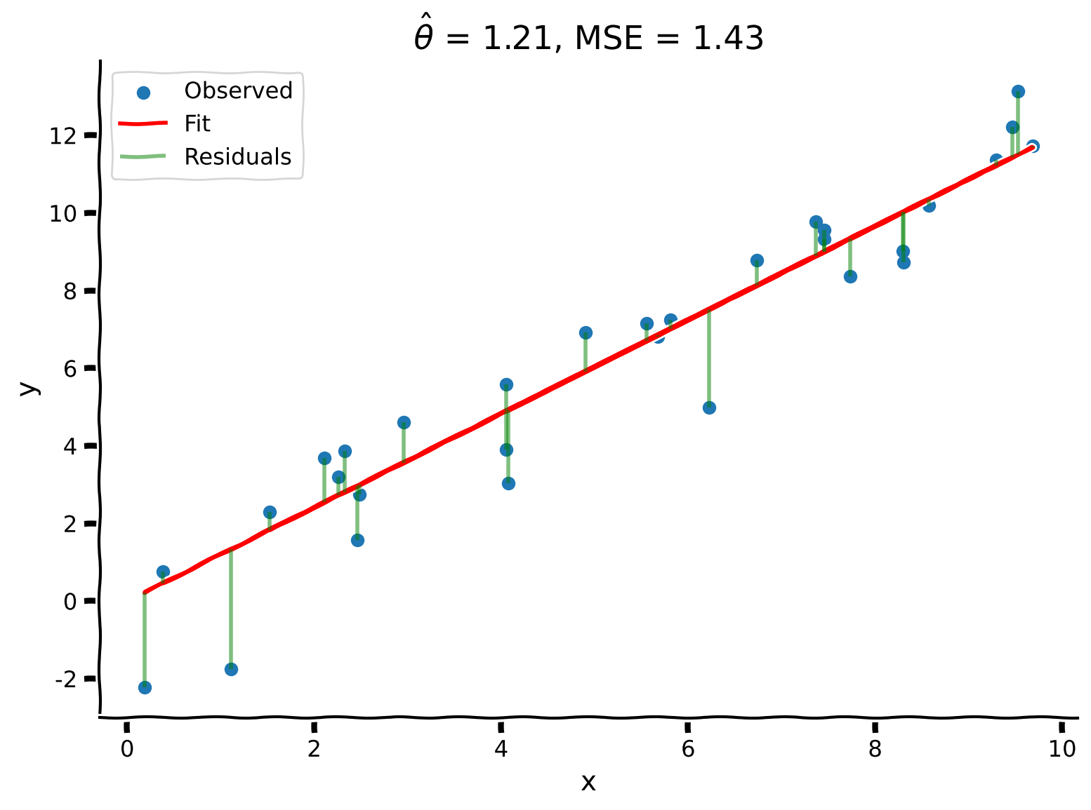
plot_observed_vs_predicted(x, y, y_hat, theta_hat)

解答を見る$

出力例:

# @title Submit your feedback
content_review(f"{feedback_prefix}_Solve_for_the_Optimal_Estimator_Exercise")

解析解は、以前のグリッドサーチよりもさらに良い結果を生み出し、$\hat{\theta} = 1.21$、$\text{MSE} = 1.43$となりました！

まとめ

チュートリアルの推定所要時間: 30分

線形最小二乗回帰はデータフィッティングに用いられる最適化手法です：

• タスク: $x_i$ が与えられたときに $y_i$ の値を予測する
• 性能指標: $\textrm{MSE}$
• 手順: 正規方程式を解くことで $\textrm{MSE}$ を最小化する

重要なポイント: モデルは目的関数を定義し、それを最小化することでフィットさせます。

補足: この場合、最小化問題には解析的な解が存在し、実際には線形代数を用いて計算できます。これは非常に強力であり、科学全般における数値計算の基盤となっています。

記法

\begin{align}
$x_{i}$ &$\quad \text{入力、独立変数}$\
$y_{i}$ &$\quad \text{観測値、従属変数}$\
$\mathbf{x}$ &$\quad \text{入力値のベクトル}$\
$\mathbf{y}$ &$\quad \text{観測値のベクトル}$\
$\hat{y}_{i}$ &$\quad \text{従属変数の推定値}$\
$\epsilon_{i}$ &$\quad \text{観測誤差}$\
$\theta$ &$\quad \text{傾きパラメータ}$\
$\hat{\theta}$ &$\quad \text{推定された傾きパラメータ}$\
$\hat{\theta}_\text{MSE}$ &$\quad \text{平均二乗誤差を用いて推定された傾きパラメータ}$\
$\textrm{MSE}$ &$\quad \text{平均二乗誤差}$\
\end{align}

ボーナス

ボーナスセクション1: 最小二乗最適化の導出

ここでは最小二乗解の導出を概説します。

まず、誤差式を $\theta$ で微分し、それをゼロに等しく設定します。

\begin{align}
$\frac{d}{d\theta}\frac{1}{N}\sum_{i=1}^N(y_i - \theta x_i)^2$ &= 0 \
$\frac{1}{N}\sum_{i=1}^N-2x_i(y_i - \theta x_i)$ &= 0
\end{align}

ここで連鎖律を用いています。これを $\theta$ について解くと、最適値は次のようになります。

ベクトル表記では次のように書けます。

これは正規方程式を解くこととして知られています。解法の詳細については、Eero Simoncelliによる最小二乗最適化のノートを参照してください。