チュートリアル 3: 「なぜ」モデル

第1週、第1日目：モデルの種類

Neuromatch Academyによる

コンテンツ作成者: Matt Laporte, Byron Galbraith, Konrad Kording

コンテンツレビュアー: Dalin Guo, Aishwarya Balwani, Madineh Sarvestani, Maryam Vaziri-Pashkam, Michael Waskom, Ella Batty

ポストプロダクションチーム: Gagana B, Spiros Chavlis

ここで使用しているデータの一部は、Steinmetz et al. (2019) が共有したデータセットのサブセットであることに感謝します。

チュートリアルの目的

推定所要時間：45分

これは神経データを理解するために使われるさまざまなタイプのモデルに関する3部構成のシリーズのチュートリアル3です。パート1と2では、データを生み出すメカニズムを探りました。このチュートリアルでは、観察されたスパイクデータがなぜそのように生成されるのかを説明できる可能性のあるモデルと手法を探ります。

異なるスパイク挙動がなぜ有益であるかを理解するために、エントロピーの概念を学びます。具体的には、以下を行います。

情報の尺度であるエントロピーの計算式をコードで実装する
いくつかの簡単な分布のエントロピーを計算する
Steinmetzデータセットのスパイク活動のエントロピーを計算する

# @title Tutorial slides
# @markdown These are the slides for the videos in all tutorials today
from IPython.display import IFrame
link_id = "6dxwe"
print(f"If you want to download the slides: https://osf.io/download/{link_id}/")
IFrame(src=f"https://mfr.ca-1.osf.io/render?url=https://osf.io/{link_id}/?direct%26mode=render%26action=download%26mode=render", width=854, height=480)

セットアップ

# @title Install and import feedback gadget


from vibecheck import DatatopsContentReviewContainer
def content_review(notebook_section: str):
    return DatatopsContentReviewContainer(
        "",  # No text prompt
        notebook_section,
        {
            "url": "https://pmyvdlilci.execute-api.us-east-1.amazonaws.com/klab",
            "name": "neuromatch_cn",
            "user_key": "y1x3mpx5",
        },
    ).render()


feedback_prefix = "W1D1_T3"

# Imports
import numpy as np
import matplotlib.pyplot as plt
from scipy import stats

# @title Figure Settings
import logging
logging.getLogger('matplotlib.font_manager').disabled = True

import ipywidgets as widgets  # interactive display
%matplotlib inline
%config InlineBackend.figure_format = 'retina'
plt.style.use("https://raw.githubusercontent.com/NeuromatchAcademy/course-content/main/nma.mplstyle")

# @title Plotting Functions

def plot_pmf(pmf,isi_range):
  """Plot the probability mass function."""
  ymax = max(0.2, 1.05 * np.max(pmf))
  pmf_ = np.insert(pmf, 0, pmf[0])
  plt.plot(bins, pmf_, drawstyle="steps")
  plt.fill_between(bins, pmf_, step="pre", alpha=0.4)
  plt.title(f"Neuron {neuron_idx}")
  plt.xlabel("Inter-spike interval (s)")
  plt.ylabel("Probability mass")
  plt.xlim(isi_range)
  plt.ylim([0, ymax])

#@title Download Data
import io
import requests
r = requests.get('https://osf.io/sy5xt/download')
if r.status_code != 200:
  print('Could not download data')
else:
  steinmetz_spikes = np.load(io.BytesIO(r.content), allow_pickle=True)['spike_times']

「なぜ」モデル

# @title Video 1: “Why” models
from ipywidgets import widgets
from IPython.display import YouTubeVideo
from IPython.display import IFrame
from IPython.display import display


class PlayVideo(IFrame):
  def __init__(self, id, source, page=1, width=400, height=300, **kwargs):
    self.id = id
    if source == 'Bilibili':
      src = f'https://player.bilibili.com/player.html?bvid={id}&page={page}'
    elif source == 'Osf':
      src = f'https://mfr.ca-1.osf.io/render?url=https://osf.io/download/{id}/?direct%26mode=render'
    super(PlayVideo, self).__init__(src, width, height, **kwargs)


def display_videos(video_ids, W=400, H=300, fs=1):
  tab_contents = []
  for i, video_id in enumerate(video_ids):
    out = widgets.Output()
    with out:
      if video_ids[i][0] == 'Youtube':
        video = YouTubeVideo(id=video_ids[i][1], width=W,
                             height=H, fs=fs, rel=0)
        print(f'Video available at https://youtube.com/watch?v={video.id}')
      else:
        video = PlayVideo(id=video_ids[i][1], source=video_ids[i][0], width=W,
                          height=H, fs=fs, autoplay=False)
        if video_ids[i][0] == 'Bilibili':
          print(f'Video available at https://www.bilibili.com/video/{video.id}')
        elif video_ids[i][0] == 'Osf':
          print(f'Video available at https://osf.io/{video.id}')
      display(video)
    tab_contents.append(out)
  return tab_contents


video_ids = [('Youtube', 'OOIDEr1e5Gg'), ('Bilibili', 'BV16t4y1Q7DR')]
tab_contents = display_videos(video_ids, W=854, H=480)
tabs = widgets.Tab()
tabs.children = tab_contents
for i in range(len(tab_contents)):
  tabs.set_title(i, video_ids[i][0])
display(tabs)

# @title Submit your feedback
content_review(f"{feedback_prefix}_Why_models_Video")

セクション1: 最適化と情報

記号の説明はまとめの後にありますので、参照してください。

ニューロンは一定時間内に発火できる回数に限りがあります。なぜならスパイクを発する行為はエネルギーを消費し、そのエネルギーは枯渇し最終的に補充されなければならないからです。下流の計算のために効果的に情報を伝達するには、ニューロンは限られた発火能力をうまく使う必要があります。これは最適化問題となります。

ニューロンが情報を伝達する能力を最大化するために、どのように発火するのが最適でしょうか？

この問いを探るために、まず情報を定量的に測る指標が必要です。シャノンはこれをエントロピーという概念で導入し、次のように定義しました。

H_b(X) = -\sum_{x\in X} p(x) \log_b p(x)

ここで、 $H$ は基数 $b$ の単位で測ったエントロピー、 $p(x)$ は事象 $x$ が全事象集合 $X$ の中で起こる確率です。詳しい導出はボーナスセクション1を参照してください。

エントロピーを測る際に最も一般的な基数は $b=2$ であり、情報量の単位はビットと呼ばれますが、他の基数も使われます（例えば $b=e$ のときはnatsと呼びます）。

まず、いくつかの単純な離散確率分布間でエントロピーがどのように変化するかを見てみましょう。このチュートリアルではこれらを確率質量関数（PMF）と呼びます。ここで $p(x_i)$ は配列の $i$ 番目の値に等しく、質量はその値に含まれる分布の割合を指します。

最初のPMFとして、分布の中央に全ての確率質量が集中しているものを選びます。

n_bins = 50  # number of points supporting the distribution
x_range = (0, 1)  # will be subdivided evenly into bins corresponding to points

bins = np.linspace(*x_range, n_bins + 1)  # bin edges

pmf = np.zeros(n_bins)
pmf[len(pmf) // 2] = 1.0  # middle point has all the mass

# Since we already have a PMF, rather than un-binned samples, `plt.hist` is not
# suitable. Instead, we directly plot the PMF as a step function to visualize
# the histogram:
pmf_ = np.insert(pmf, 0, pmf[0])  # this is necessary to align plot steps with bin edges
plt.plot(bins, pmf_, drawstyle="steps")
# `fill_between` provides area shading
plt.fill_between(bins, pmf_, step="pre", alpha=0.4)
plt.xlabel("x")
plt.ylabel("p(x)")
plt.xlim(x_range)
plt.ylim(0, 1)
plt.show()

この分布からサンプルを取ると、毎回何が得られるか正確にわかっています。全ての質量が単一の事象に集中している分布は決定的と呼ばれます。

決定的分布のエントロピーはどれくらいでしょうか？次の演習で計算してみましょう。

コーディング演習1: エントロピーの計算

最初の演習は、離散確率分布の質量関数が与えられたときにエントロピーを計算するメソッドを実装することです。エントロピーは_ビット_単位で求めたいので、適切な対数関数を使うことを忘れないでください。

$\log(0)$ は定義されていません。NumPyの対数関数（例えばnp.log2）は0のときnp.nan（「数値ではない」）を返します。慣例として、質量がゼロの点に対応するこれらの未定義項はエントロピー計算の和から除外します。

def entropy(pmf):
  """Given a discrete distribution, return the Shannon entropy in bits.

  This is a measure of information in the distribution. For a totally
  deterministic distribution, where samples are always found in the same bin,
  then samples from the distribution give no more information and the entropy
  is 0.

  For now this assumes `pmf` arrives as a well-formed distribution (that is,
  `np.sum(pmf)==1` and `not np.any(pmf < 0)`)

  Args:
    pmf (np.ndarray): The probability mass function for a discrete distribution
      represented as an array of probabilities.
  Returns:
    h (number): The entropy of the distribution in `pmf`.

  """
  ############################################################################
  # Exercise for students: compute the entropy of the provided PMF
  #   1. Exclude the points in the distribution with no mass (where `pmf==0`).
  #      Hint: this is equivalent to including only the points with `pmf>0`.
  #   2. Implement the equation for Shannon entropy (in bits).
  #  When ready to test, comment or remove the next line
  raise NotImplementedError("Exercise: implement the equation for entropy")
  ############################################################################

  # reduce to non-zero entries to avoid an error from log2(0)
  pmf = ...

  # implement the equation for Shannon entropy (in bits)
  h = ...

  # return the absolute value (avoids getting a -0 result)
  return np.abs(h)

# Call entropy function and print result
print(f"{entropy(pmf):.2f} bits")

解答を見る$

# @title Submit your feedback
content_review(f"{feedback_prefix}_Optimization_and_Information_Exercise")

決定的分布からは驚きはゼロと予想されます。手計算で行うと単に $-1\log_2 1 = -0=0$ となります。

ピークの位置（つまり全質量がある点やビン）を変えてもエントロピーは変わりません。エントロピーは分布に対してサンプルがどれだけ予測可能かを表します。単一のピークはどの点にあっても決定的であり、次の図はエントロピーがゼロとなるPMFの例です。

# @markdown Execute this cell to visualize another PMF with zero entropy
pmf = np.zeros(n_bins)
pmf[2] = 1.0  # arbitrary point has all the mass

pmf_ = np.insert(pmf, 0, pmf[0])
plt.plot(bins, pmf_, drawstyle="steps")
plt.fill_between(bins, pmf_, step="pre", alpha=0.4)
plt.xlabel("x")
plt.ylabel("p(x)")
plt.xlim(x_range)
plt.ylim(0, 1);

では、質量が2つの点に均等に分かれている分布はどうでしょうか？

# @markdown Execute this cell to visualize a PMF with split mass

pmf = np.zeros(n_bins)
pmf[len(pmf) // 3] = 0.5
pmf[2 * len(pmf) // 3] = 0.5

pmf_ = np.insert(pmf, 0, pmf[0])
plt.plot(bins, pmf_, drawstyle="steps")
plt.fill_between(bins, pmf_, step="pre", alpha=0.4)
plt.xlabel("x")
plt.ylabel("p(x)")
plt.xlim(x_range)
plt.ylim(0, 1)
plt.show()

この場合のエントロピー計算は： $-(0.5 \log_2 0.5 + 0.5\log_2 0.5)=1$

エントロピーは1ビットです。これはランダムサンプルを取る前に、サンプルが分布のどちらのピークに落ちるかについて1ビットの不確実性があることを意味します。すなわち、最初のピークか2番目のピークのどちらかです。

同様に、ピークの一方を高く（その点により多くの確率質量がある）し、もう一方を低くすると、サンプルがどちらかの点に落ちる確実性が増すためエントロピーは減少します： $-(0.2 \log_2 0.2 + 0.8\log_2 0.8)\approx 0.72$

ピークの数や重み付けを変えて、エントロピーがどのように変化するか試してみてください。

質量をさらに多くの点に分けると、エントロピーは増加し続けます。 $N$ 個の点に均等に分布する場合、 $p_i=p=1/N$ として一般形を導きましょう：

\begin{align}
- $\sum_i p_i \log_b p_i$ &= - $\sum_i^N \frac{1}{N} \log_b \frac{1}{N}$ \
&= - $\log_b \frac{1}{N}$ \
&= $\log_b N \end{align}$

$N$ 個の離散点がある場合、一様分布（すべての点が等しい質量を持つ）は最大のエントロピーを持つ分布であり、その値は $\log_b N$ です。このエントロピーの上限はビニング戦略を考える際に有用で、 $N$ 個の離散点（またはビン）に対するエントロピーの推定値は区間 $[0, \log_b N]$ 内にある必要があります。

# @markdown Execute this cell to visualize a PMF of uniform distribution

pmf = np.ones(n_bins) / n_bins  # [1/N] * N

pmf_ = np.insert(pmf, 0, pmf[0])
plt.plot(bins, pmf_, drawstyle="steps")
plt.fill_between(bins, pmf_, step="pre", alpha=0.4)
plt.xlabel("x")
plt.ylabel("p(x)")
plt.xlim(x_range)
plt.ylim(0, 1)
plt.show()

ここでは、50個の点があり、一様分布のエントロピーは $\log_2 50\approx 5.64$ です。もし50個の点（またはビン）に対して_任意の_離散分布 $X$ を構築し、そのエントロピー $H_2(X)>\log_2 50$ と計算された場合、離散エントロピー計算の実装に何か問題があるはずです。

セクション 2: 情報、ニューロン、スパイク

チュートリアル開始からここまでの推定所要時間: 20分

# @title Video 2: Entropy of different distributions
from ipywidgets import widgets
from IPython.display import YouTubeVideo
from IPython.display import IFrame
from IPython.display import display


class PlayVideo(IFrame):
  def __init__(self, id, source, page=1, width=400, height=300, **kwargs):
    self.id = id
    if source == 'Bilibili':
      src = f'https://player.bilibili.com/player.html?bvid={id}&page={page}'
    elif source == 'Osf':
      src = f'https://mfr.ca-1.osf.io/render?url=https://osf.io/download/{id}/?direct%26mode=render'
    super(PlayVideo, self).__init__(src, width, height, **kwargs)


def display_videos(video_ids, W=400, H=300, fs=1):
  tab_contents = []
  for i, video_id in enumerate(video_ids):
    out = widgets.Output()
    with out:
      if video_ids[i][0] == 'Youtube':
        video = YouTubeVideo(id=video_ids[i][1], width=W,
                             height=H, fs=fs, rel=0)
        print(f'Video available at https://youtube.com/watch?v={video.id}')
      else:
        video = PlayVideo(id=video_ids[i][1], source=video_ids[i][0], width=W,
                          height=H, fs=fs, autoplay=False)
        if video_ids[i][0] == 'Bilibili':
          print(f'Video available at https://www.bilibili.com/video/{video.id}')
        elif video_ids[i][0] == 'Osf':
          print(f'Video available at https://osf.io/{video.id}')
      display(video)
    tab_contents.append(out)
  return tab_contents


video_ids = [('Youtube', 'o6nyrx3KH20'), ('Bilibili', 'BV1df4y1976g')]
tab_contents = display_videos(video_ids, W=854, H=480)
tabs = widgets.Tab()
tabs.children = tab_contents
for i in range(len(tab_contents)):
  tabs.set_title(i, video_ids[i][0])
display(tabs)

# @title Submit your feedback
content_review(f"{feedback_prefix}_Entropy_of_different_distributions_Video")

チュートリアル1でのスパイク時間とスパイク間隔（ISI）の議論を思い出してください。これらの測定値の情報量（または分布エントロピー）は、神経系の理論について何を示しているでしょうか？

同じ平均ISIを持つが異なる分布を持つ3つの仮想ニューロンを考えます：

決定論的
一様分布
指数分布

ISI分布の平均を固定することは、その逆数であるニューロンの平均発火率を固定することと同じです。もしニューロンが固定されたエネルギー予算を持ち、各スパイクが同じエネルギーコストを持つなら、平均発火率を固定することでエネルギー消費を正規化しています。これにより、異なるISI分布のエントロピーを比較する基準が得られます。言い換えれば、ニューロンが固定された予算を持つ場合、（他の条件が同じなら）出力の情報量を最大化するためにどのISI分布を表現すべきでしょうか？

3つの分布を構築し、それらのエントロピーがどのように異なるかを見てみましょう。

n_bins = 50
mean_isi = 0.025
isi_range = (0, 0.25)

bins = np.linspace(*isi_range, n_bins + 1)
mean_idx = np.searchsorted(bins, mean_isi)

# 1. all mass concentrated on the ISI mean
pmf_single = np.zeros(n_bins)
pmf_single[mean_idx] = 1.0

# 2. mass uniformly distributed about the ISI mean
pmf_uniform = np.zeros(n_bins)
pmf_uniform[0:2*mean_idx] = 1 / (2 * mean_idx)

# 3. mass exponentially distributed about the ISI mean
pmf_exp = stats.expon.pdf(bins[1:], scale=mean_isi)
pmf_exp /= np.sum(pmf_exp)

# @markdown Run this cell to plot the three PMFs
fig, axes = plt.subplots(ncols=3, figsize=(15, 5))

dists =  [# (subplot title, pmf, ylim)
          ("(1) Deterministic", pmf_single, (0, 1.05)),
          ("(1) Uniform", pmf_uniform, (0, 1.05)),
          ("(1) Exponential", pmf_exp, (0, 1.05))]

for ax, (label, pmf_, ylim) in zip(axes, dists):
  pmf_ = np.insert(pmf_, 0, pmf_[0])
  ax.plot(bins, pmf_, drawstyle="steps")
  ax.fill_between(bins, pmf_, step="pre", alpha=0.4)
  ax.set_title(label)
  ax.set_xlabel("Inter-spike interval (s)")
  ax.set_ylabel("Probability mass")
  ax.set_xlim(isi_range)
  ax.set_ylim(ylim)
plt.show()

print(
  f"Deterministic: {entropy(pmf_single):.2f} bits",
  f"Uniform: {entropy(pmf_uniform):.2f} bits",
  f"Exponential: {entropy(pmf_exp):.2f} bits",
  sep="\n",
)

セクション 3: データからISI分布のエントロピーを計算する

チュートリアル開始からここまでの推定所要時間: 25分

セクション 3.1: ヒストグラムから確率を計算する

# @title Video 3: Probabilities from histogram
from ipywidgets import widgets
from IPython.display import YouTubeVideo
from IPython.display import IFrame
from IPython.display import display


class PlayVideo(IFrame):
  def __init__(self, id, source, page=1, width=400, height=300, **kwargs):
    self.id = id
    if source == 'Bilibili':
      src = f'https://player.bilibili.com/player.html?bvid={id}&page={page}'
    elif source == 'Osf':
      src = f'https://mfr.ca-1.osf.io/render?url=https://osf.io/download/{id}/?direct%26mode=render'
    super(PlayVideo, self).__init__(src, width, height, **kwargs)


def display_videos(video_ids, W=400, H=300, fs=1):
  tab_contents = []
  for i, video_id in enumerate(video_ids):
    out = widgets.Output()
    with out:
      if video_ids[i][0] == 'Youtube':
        video = YouTubeVideo(id=video_ids[i][1], width=W,
                             height=H, fs=fs, rel=0)
        print(f'Video available at https://youtube.com/watch?v={video.id}')
      else:
        video = PlayVideo(id=video_ids[i][1], source=video_ids[i][0], width=W,
                          height=H, fs=fs, autoplay=False)
        if video_ids[i][0] == 'Bilibili':
          print(f'Video available at https://www.bilibili.com/video/{video.id}')
        elif video_ids[i][0] == 'Osf':
          print(f'Video available at https://osf.io/{video.id}')
      display(video)
    tab_contents.append(out)
  return tab_contents


video_ids = [('Youtube', 'e2U_-07O9jo'), ('Bilibili', 'BV1Jk4y1B7cz')]
tab_contents = display_videos(video_ids, W=854, H=480)
tabs = widgets.Tab()
tabs.children = tab_contents
for i in range(len(tab_contents)):
  tabs.set_title(i, video_ids[i][0])
display(tabs)

# @title Submit your feedback
content_review(f"{feedback_prefix}_Probabilities_from_histogram_Video")

前の例では、理想化されたシナリオを示すためにPMFを手作業で作成しました。実際のニューロンから記録されたデータからこれらをどのように計算するでしょうか？

一つの方法は、以前に計算したISIヒストグラムを次の式を使って離散確率分布に変換することです：

p_i = \frac{n_i}{\sum\nolimits_{i}n_i}

ここで、 $p_i$ は特定の区間 $i$ にISIが入る確率、 $n_i$ はその区間で観測されたISIの数です。

コーディング演習 3.1: 確率質量関数

2つ目の演習は、ISIビンのカウント配列から確率質量関数を生成するメソッドを実装することです。

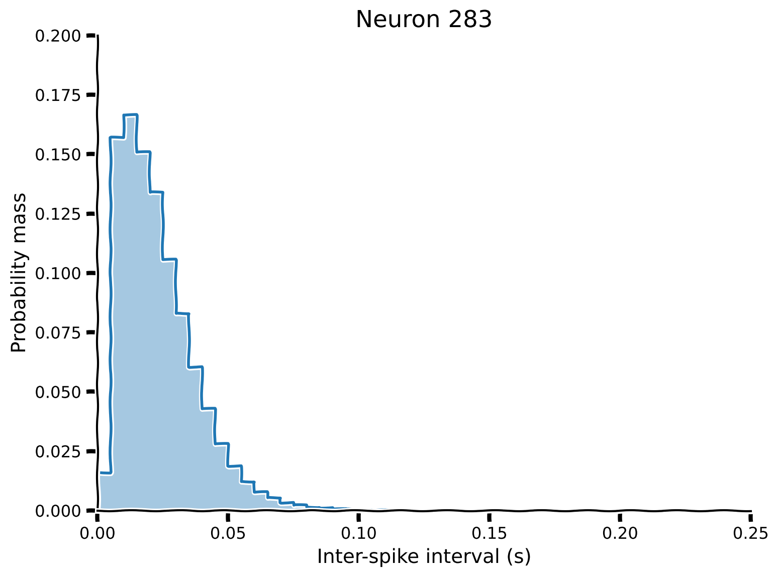
解答の検証には、Steinmetzデータセットから取得した実際の神経データのISI確率分布を計算します。

def pmf_from_counts(counts):
  """Given counts, normalize by the total to estimate probabilities."""
  ###########################################################################
  # Exercise: Compute the PMF. Remove the next line to test your function
  raise NotImplementedError("Student exercise: compute the PMF from ISI counts")
  ###########################################################################

  pmf = ...

  return pmf


# Get neuron index
neuron_idx = 283

# Get counts of ISIs from Steinmetz data
isi = np.diff(steinmetz_spikes[neuron_idx])
bins = np.linspace(*isi_range, n_bins + 1)
counts, _ = np.histogram(isi, bins)

# Compute pmf
pmf = pmf_from_counts(counts)

# Visualize
plot_pmf(pmf, isi_range)

解答を見る$

出力例:

# @title Submit your feedback
content_review(f"{feedback_prefix}_Probability_mass_function_Exercise")

セクション 3.2: pmfからエントロピーを計算する

# @title Video 4: Calculating entropy from pmf
from ipywidgets import widgets
from IPython.display import YouTubeVideo
from IPython.display import IFrame
from IPython.display import display


class PlayVideo(IFrame):
  def __init__(self, id, source, page=1, width=400, height=300, **kwargs):
    self.id = id
    if source == 'Bilibili':
      src = f'https://player.bilibili.com/player.html?bvid={id}&page={page}'
    elif source == 'Osf':
      src = f'https://mfr.ca-1.osf.io/render?url=https://osf.io/download/{id}/?direct%26mode=render'
    super(PlayVideo, self).__init__(src, width, height, **kwargs)


def display_videos(video_ids, W=400, H=300, fs=1):
  tab_contents = []
  for i, video_id in enumerate(video_ids):
    out = widgets.Output()
    with out:
      if video_ids[i][0] == 'Youtube':
        video = YouTubeVideo(id=video_ids[i][1], width=W,
                             height=H, fs=fs, rel=0)
        print(f'Video available at https://youtube.com/watch?v={video.id}')
      else:
        video = PlayVideo(id=video_ids[i][1], source=video_ids[i][0], width=W,
                          height=H, fs=fs, autoplay=False)
        if video_ids[i][0] == 'Bilibili':
          print(f'Video available at https://www.bilibili.com/video/{video.id}')
        elif video_ids[i][0] == 'Osf':
          print(f'Video available at https://osf.io/{video.id}')
      display(video)
    tab_contents.append(out)
  return tab_contents


video_ids = [('Youtube', 'Xjy-jj-6Oz0'), ('Bilibili', 'BV1vA411e7Cd')]
tab_contents = display_videos(video_ids, W=854, H=480)
tabs = widgets.Tab()
tabs.children = tab_contents
for i in range(len(tab_contents)):
  tabs.set_title(i, video_ids[i][0])
display(tabs)

# @title Submit your feedback
content_review(f"{feedback_prefix}_Calculating_entropy_from_pmf_Video")

実際のニューロンのスパイク活動の確率分布が得られたので、そのエントロピーを計算できます。

print(f"Entropy for Neuron {neuron_idx}: {entropy(pmf):.2f} bits")

インタラクティブデモ 3.2: ニューロンのエントロピー

上記の分布プロットとエントロピー計算をインタラクティブなウィジェットと組み合わせて、データセット内の異なるニューロンがどのようにスパイク活動や相対情報量に違いがあるかを探れます。ニューロン間の平均発火率は固定されていないため、均一なISI分布を持つニューロンの方が、より指数分布的なニューロンよりも高いエントロピーを持つ場合があることに注意してください。

# @markdown **Run the cell** to enable the sliders.

def _pmf_from_counts(counts):
  """Given counts, normalize by the total to estimate probabilities."""
  pmf = counts / np.sum(counts)
  return pmf


def _entropy(pmf):
  """Given a discrete distribution, return the Shannon entropy in bits."""
  # remove non-zero entries to avoid an error from log2(0)
  pmf = pmf[pmf > 0]
  h = -np.sum(pmf * np.log2(pmf))
  # absolute value applied to avoid getting a -0 result
  return np.abs(h)


@widgets.interact(neuron=widgets.IntSlider(0, min=0, max=(len(steinmetz_spikes)-1)))
def steinmetz_pmf(neuron):
  """ Given a neuron from the Steinmetz data, compute its PMF and entropy """
  isi = np.diff(steinmetz_spikes[neuron])
  bins = np.linspace(*isi_range, n_bins + 1)
  counts, _ = np.histogram(isi, bins)
  pmf = _pmf_from_counts(counts)

  plot_pmf(pmf, isi_range)
  plt.title(f"Neuron {neuron}: H = {_entropy(pmf):.2f} bits")
  plt.show()

# @title Submit your feedback
content_review(f"{feedback_prefix}_Entropy_of_neurons_Interactive_Demo")

セクション4: なぜモデルなのかを考える

チュートリアル開始からここまでの推定時間: 35分

考えよう！3: なぜモデルなのかを考える

以下の質問について、グループで約10分間話し合ってください：

なぜモデルを見たことがありますか？
なぜモデルを作ったことがありますか？
なぜモデルは役に立つのでしょうか？
いつモデルは可能でしょうか？あなたの分野にはなぜモデルがありますか？
なぜモデルを構築することで何が学べますか？

# @title Submit your feedback
content_review(f"{feedback_prefix}_Reflecting_on_why_models_Discussion")

まとめ

チュートリアルの推定所要時間: 45分

# @title Video 5: Summary of model types
from ipywidgets import widgets
from IPython.display import YouTubeVideo
from IPython.display import IFrame
from IPython.display import display


class PlayVideo(IFrame):
  def __init__(self, id, source, page=1, width=400, height=300, **kwargs):
    self.id = id
    if source == 'Bilibili':
      src = f'https://player.bilibili.com/player.html?bvid={id}&page={page}'
    elif source == 'Osf':
      src = f'https://mfr.ca-1.osf.io/render?url=https://osf.io/download/{id}/?direct%26mode=render'
    super(PlayVideo, self).__init__(src, width, height, **kwargs)


def display_videos(video_ids, W=400, H=300, fs=1):
  tab_contents = []
  for i, video_id in enumerate(video_ids):
    out = widgets.Output()
    with out:
      if video_ids[i][0] == 'Youtube':
        video = YouTubeVideo(id=video_ids[i][1], width=W,
                             height=H, fs=fs, rel=0)
        print(f'Video available at https://youtube.com/watch?v={video.id}')
      else:
        video = PlayVideo(id=video_ids[i][1], source=video_ids[i][0], width=W,
                          height=H, fs=fs, autoplay=False)
        if video_ids[i][0] == 'Bilibili':
          print(f'Video available at https://www.bilibili.com/video/{video.id}')
        elif video_ids[i][0] == 'Osf':
          print(f'Video available at https://osf.io/{video.id}')
      display(video)
    tab_contents.append(out)
  return tab_contents


video_ids = [('Youtube', 'X4K2RR5qBK8'), ('Bilibili', 'BV1F5411e7ww')]
tab_contents = display_videos(video_ids, W=854, H=480)
tabs = widgets.Tab()
tabs.children = tab_contents
for i in range(len(tab_contents)):
  tabs.set_title(i, video_ids[i][0])
display(tabs)

# @title Submit your feedback
content_review(f"{feedback_prefix}_Summary_of_model_types_Video")

おめでとうございます！最初のNMAチュートリアルを終了しました。この3部構成のチュートリアルシリーズでは、さまざまなタイプのモデルを使って、Steinmetzデータセットで記録されたニューロンのスパイク挙動を理解しました。

「何を」モデルを使って、実際のニューロンのISI分布が指数分布に最も近いことを発見しました
「どのように」モデルを使って、バランスの取れた興奮性および抑制性入力とリーキ膜が、指数分布的なISI分布を示すニューロンスパイクを生み出すことを発見しました
「なぜ」モデルを使って、平均スパイク数が制約されているときに指数ISI分布が最も情報量が多いことを発見しました

記法

\begin{align}
H(X) & $\quad \text{ランダム変数Xのエントロピー}$ \
b & $\quad \text{底、例: b=2 または b=e}$ \
x & $\quad \text{事象 x}$ \
p(x) & $\quad \text{事象 x が観測される確率}$ \
$\text{ISI}$ & $\quad \text{インタースパイク間隔}$ \
$n_i$ & $\quad \text{区間 i に観測されたISIのカウント}$ \
$p_i$ & $\quad \text{特定の区間 i にISIが入る確率} \end{align}$

ボーナス

ボーナスセクション1: エントロピーの基礎

情報理論の基礎となる1948年の論文$で、クロード・シャノンは確率質量 $p_i\in p(X)$ が離散的に分布する点 $x_i\in X$ に対して、エントロピーを定義する関数 $H$ に対して3つの条件を提示しました：

$H$ は $p_i$ に関して連続であること。

つまり、 $H$ は各点 $x_i$ の質量 $p_i$ が滑らかに変化したときに滑らかに変化するべきです。

すべての点が等しい確率質量を持つ場合、 $p_i=1/N$ 、 $H$ は $N$ の非減少関数であること。

つまり、 $X_N$ が $N$ 個の離散点を持つ支持集合で、 $p(x\in X_N)$ が各点に一定の質量を割り当てるなら、 $H(X_1) < H(X_2) < H(X_3) < \dots$ となるべきです。

$H$ は分布の同等な（分解・合成）操作に対して不変であること。

例えば（シャノンの論文から）、質量が $(\frac{1}{2},\frac{1}{3},\frac{1}{6})$ の3点の離散分布があるとき、そのエントロピーは3点の直接選択として $H(\frac{1}{2},\frac{1}{3},\frac{1}{6})$ として計算できます。しかし、2段階の選択としても表現できます：
1. 質量 $1/2$ の点をサンプリングするかどうか（しない は残りの $1/2$ で、その細分は最初の選択には含まれません）、
2. もし（確率 $1/2$ で）最初の点をサンプリングしなければ、残りの2点（質量 $1/3$ と $1/6$ ）のどちらかをサンプリングします。
この場合、 $H(\frac{1}{2},\frac{1}{3},\frac{1}{6})=H(\frac{1}{2},\frac{1}{2}) + \frac{1}{2}H(\frac{1}{3}, \frac{1}{6})$ である必要があります。

これら3つの条件を満たす関数は（線形スケーリングを除いて）唯一つ存在します：

H_b(X) = -\sum_{x\in X} p(x) \log_b p(x)

ここで対数の底 $b>1$ はエントロピーの単位を決定します。最も一般的なものは、 $b=2$ （ビット単位）と $b=e$ （ナット単位）です。

この関数は分布における自己情報の期待値として見ることができます：

\begin{align}
$H_b(X)$ &= $\mathbb{E}_{x\in X} \left$ [ $I_b(x)$ $\right$ ]\
$I_b(x)$ &= - $\log_b p(x) \end{align}$

自己情報は確率の負の対数であり、分布からサンプリングされた事象がどれだけ驚くべきかの尺度です。 $p(x)=1$ の事象は確実に起こるため、その自己情報はゼロ（それらが構成する分布のエントロピーもゼロ）であり、全く驚くべきではありません。事象の確率が小さいほど自己情報は大きくなり、その事象を観測することはより驚くべきことになります。