![]()

チュートリアル 2: 「どのように」モデル
第1週、第1日目: モデルの種類
Neuromatch Academyによる
コンテンツ作成者: Matt Laporte, Byron Galbraith, Konrad Kording
コンテンツレビュアー: Dalin Guo, Aishwarya Balwani, Madineh Sarvestani, Maryam Vaziri-Pashkam, Michael Waskom, Ella Batty
制作編集者: Gagana B, Spiros Chavlis
チュートリアルの目的
チュートリアルの推定所要時間: 45分
これは神経データを理解するために使われるさまざまなタイプのモデルに関する3部構成のシリーズの第2回目です。このチュートリアルでは、観察されたスパイクデータがどのように生成されるかを説明できる可能性のあるモデルを探ります。
チュートリアル1で保存した神経データが生じるメカニズムを理解するために、単純な神経モデルを構築し、そのスパイク応答を実際のデータと比較します。具体的には:
- 単純な「リーキー積分発火」ニューロンモデルをシミュレートするコードを書く
- モデルをより複雑に、しかしより生理学的にリアルにするために詳細を追加する
# @title Tutorial slides
# @markdown These are the slides for the videos in all tutorials today
from IPython.display import IFrame
link_id = "6dxwe"
print(f"If you want to download the slides: https://osf.io/download/{link_id}/")
IFrame(src=f"https://mfr.ca-1.osf.io/render?url=https://osf.io/{link_id}/?direct%26mode=render%26action=download%26mode=render", width=854, height=480)
セットアップ
# @title Install and import feedback gadget


from vibecheck import DatatopsContentReviewContainer
def content_review(notebook_section: str):
    return DatatopsContentReviewContainer(
        "",  # No text prompt
        notebook_section,
        {
            "url": "https://pmyvdlilci.execute-api.us-east-1.amazonaws.com/klab",
            "name": "neuromatch_cn",
            "user_key": "y1x3mpx5",
        },
    ).render()


feedback_prefix = "W1D1_T2"
import numpy as np
import matplotlib.pyplot as plt
from scipy import stats# @title Figure Settings
import logging
logging.getLogger('matplotlib.font_manager').disabled = True
import ipywidgets as widgets # interactive display
%matplotlib inline
%config InlineBackend.figure_format = 'retina'
plt.style.use("https://raw.githubusercontent.com/NeuromatchAcademy/course-content/main/nma.mplstyle")# @title Plotting Functions
def histogram(counts, bins, vlines=(), ax=None, ax_args=None, **kwargs):
"""Plot a step histogram given counts over bins."""
if ax is None:
_, ax = plt.subplots()
# duplicate the first element of `counts` to match bin edges
counts = np.insert(counts, 0, counts[0])
ax.fill_between(bins, counts, step="pre", alpha=0.4, **kwargs) # area shading
ax.plot(bins, counts, drawstyle="steps", **kwargs) # lines
for x in vlines:
ax.axvline(x, color='r', linestyle='dotted') # vertical line
if ax_args is None:
ax_args = {}
# heuristically set max y to leave a bit of room
ymin, ymax = ax_args.get('ylim', [None, None])
if ymax is None:
ymax = np.max(counts)
if ax_args.get('yscale', 'linear') == 'log':
ymax *= 1.5
else:
ymax *= 1.1
if ymin is None:
ymin = 0
if ymax == ymin:
ymax = None
ax_args['ylim'] = [ymin, ymax]
ax.set(**ax_args)
ax.autoscale(enable=False, axis='x', tight=True)
def plot_neuron_stats(v, spike_times):
fig, (ax1, ax2) = plt.subplots(ncols=2, figsize=(12, 5))
# membrane voltage trace
ax1.plot(v[0:100])
ax1.set(xlabel='Time', ylabel='Voltage')
# plot spike events
for x in spike_times:
if x >= 100:
break
ax1.axvline(x, color='red')
# ISI distribution
if len(spike_times)>1:
isi = np.diff(spike_times)
n_bins = np.arange(isi.min(), isi.max() + 2) - .5
counts, bins = np.histogram(isi, n_bins)
vlines = []
if len(isi) > 0:
vlines = [np.mean(isi)]
xmax = max(20, int(bins[-1])+5)
histogram(counts, bins, vlines=vlines, ax=ax2, ax_args={
'xlabel': 'Inter-spike interval',
'ylabel': 'Number of intervals',
'xlim': [0, xmax]
})
else:
ax2.set(xlabel='Inter-spike interval',
ylabel='Number of intervals')
plt.show()「どのように」モデル
# @title Video 1: "How" models
from ipywidgets import widgets
from IPython.display import YouTubeVideo
from IPython.display import IFrame
from IPython.display import display


class PlayVideo(IFrame):
  def __init__(self, id, source, page=1, width=400, height=300, **kwargs):
    self.id = id
    if source == 'Bilibili':
      src = f'https://player.bilibili.com/player.html?bvid={id}&page={page}'
    elif source == 'Osf':
      src = f'https://mfr.ca-1.osf.io/render?url=https://osf.io/download/{id}/?direct%26mode=render'
    super(PlayVideo, self).__init__(src, width, height, **kwargs)


def display_videos(video_ids, W=400, H=300, fs=1):
  tab_contents = []
  for i, video_id in enumerate(video_ids):
    out = widgets.Output()
    with out:
      if video_ids[i][0] == 'Youtube':
        video = YouTubeVideo(id=video_ids[i][1], width=W,
                             height=H, fs=fs, rel=0)
        print(f'Video available at https://youtube.com/watch?v={video.id}')
      else:
        video = PlayVideo(id=video_ids[i][1], source=video_ids[i][0], width=W,
                          height=H, fs=fs, autoplay=False)
        if video_ids[i][0] == 'Bilibili':
          print(f'Video available at https://www.bilibili.com/video/{video.id}')
        elif video_ids[i][0] == 'Osf':
          print(f'Video available at https://osf.io/{video.id}')
      display(video)
    tab_contents.append(out)
  return tab_contents


video_ids = [('Youtube', 'PpnagITsb3E'), ('Bilibili', 'BV1yV41167Di')]
tab_contents = display_videos(video_ids, W=854, H=480)
tabs = widgets.Tab()
tabs.children = tab_contents
for i in range(len(tab_contents)):
  tabs.set_title(i, video_ids[i][0])
display(tabs)
# @title Submit your feedback
content_review(f"{feedback_prefix}_How_models_Video")セクション1: 線形積分発火ニューロン
リーキー積分発火ニューロンを記述するためにいくつかの数学を使います。もし記号の意味(例えば特定の変数名が何を表すか)をすぐに確認したい場合は、まとめの後の記号セクションを参照してください。
ニューロンはどのようにスパイクするのでしょうか?
ニューロンは細胞膜をまたいで電場を充電・放電します。この電場の状態は膜電位で表されます。膜電位はニューロンの興奮によって上昇し、閾値に達するとスパイクが発生します。膜電位はリセットされ、次のスパイクが発生するまで再び閾値に達する必要があります。
スパイクするニューロンの最も単純なモデルの一つが線形積分発火モデルです。このモデルでは、ニューロンは興奮性入力電流 に比例した係数 をかけたものに応じて膜電位 を時間とともに増加させます:
が閾値に達するとスパイクが発生し、 は初期値にリセットされ、このプロセスが続きます。
ここでは、開始電位と閾値をそれぞれ と とします。例えば、 が一定(つまり入力電流が一定)であれば、 となり、各タイムステップで膜電位 は ずつ増加し、 タイムステップ後に閾値に達して にリセットされます。
膜電位 はスカラー、つまり単一の実数(浮動小数点数)として定義しています。しかし、生物学的なニューロンの膜電位は、ある時点で細胞膜のすべての場所で正確に一定ではありません。この変動をより複雑なモデル(例えば複数の数値を使う)で表現することも可能です。果たしてそれは必要でしょうか?
提案したモデルは1次元の単純化です。実際のニューロンの複雑な構造や動態の異なる部分を保持するために多くの詳細を追加できます。膜電位の小さな局所的な変化に興味がある場合、この1次元単純化は問題になるかもしれません。しかし、ここでは理想化された「点」ニューロンモデルを仮定します。
スパイク入力
単純化したニューロンダイナミクスのモデルを考えた上で、入力 がどのような形を取るかを考える必要があります。モデルニューロンに入力を与えるシナプス前ニューロンの発火挙動をどのように指定すればよいでしょうか?
上の単純な例()とは異なり、入力電流は一般に一定ではありません。物理的な入力は時間とともに変動します。この変動は分布で表現できます。
1タイムステップあたりの入力電流 は、非負整数()の入力スパイク数の等しい寄与の合計と仮定します。モデルニューロンはあるタイムステップで3つの入力スパイクから電流を積分し、次のタイムステップでは7つのスパイクから積分するかもしれません。分布からサンプリングした場合も同様の挙動が見られるはずです。
入力ニューロンについて他に情報がない場合、分布は平均(すなわち平均発火率、または1タイムステップあたりに受け取るスパイク数)を持ち、入力ニューロンのスパイクイベントは時間的に独立であると仮定します。これらは実際のニューロンの文脈で妥当な仮定でしょうか?
これらの仮定の下で適切な分布はポアソン分布であり、これを用いて をモデル化します:
ここで は分布の平均、すなわち1タイムステップあたりの平均スパイク数です。
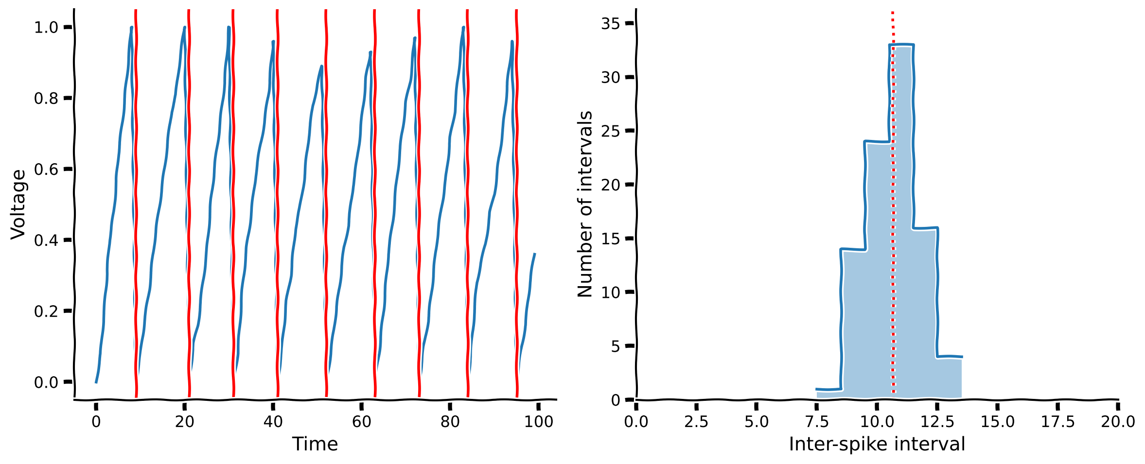
コーディング演習1: の計算
最初の演習では、線形積分発火モデルニューロンの電圧変化 (1タイムステップあたり)を計算するコードを書きます。数値積分を扱う残りのコードは提供されているので、lif_neuron 関数内で dv の定義を埋めるだけで構いません。ポアソン乱数のパラメータ は関数引数 rate で与えられます。
scipy.stats パッケージはさまざまな確率分布の操作やサンプリングに便利です。ここでは scipy.stats.poisson クラスとそのメソッド rvs を使ってポアソン分布に従う乱数を生成します。このチュートリアルではこのパッケージを stats という別名でインポートしているので、コード内では stats.poisson として参照してください。
def lif_neuron(n_steps=1000, alpha=0.01, rate=10):
  """ Simulate a linear integrate-and-fire neuron.

  Args:
    n_steps (int): The number of time steps to simulate the neuron's activity.
    alpha (float): The input scaling factor
    rate (int): The mean rate of incoming spikes

  """
  # Precompute Poisson samples for speed
  exc = stats.poisson(rate).rvs(n_steps)

  # Initialize voltage and spike storage
  v = np.zeros(n_steps)
  spike_times = []

  ################################################################################
  # Students: compute dv, then comment out or remove the next line
  raise NotImplementedError("Exercise: compute the change in membrane potential")
  ################################################################################

  # Loop over steps
  for i in range(1, n_steps):

    # Update v
    dv = ...
    v[i] = v[i-1] + dv

    # If spike happens, reset voltage and record
    if v[i] > 1:
      spike_times.append(i)
      v[i] = 0

  return v, spike_times

# Set random seed (for reproducibility)
np.random.seed(12)

# Model LIF neuron
v, spike_times = lif_neuron()

# Visualize
plot_neuron_stats(v, spike_times)出力例:
# @title Submit your feedback
content_review(f"{feedback_prefix}_Compute_dVm_Exercise")
インタラクティブデモ1: 線形IFニューロン
前回と同様に、LIFモデルのさまざまなパラメータがISI分布にどのように影響するかを探索できます。具体的には、入力スケーリング係数 alpha と入力スパイクの平均発火率 rate を変化させられます。
- このモデルのスパイクパターンはどのようなものですか?
alphaを上げたり下げたりするとどんな影響がありますか?rateを上げたり下げたりするとどんな影響がありますか?- ISIの分布はチュートリアル1で観察したデータの分布に似ていますか?
# @markdown You don't need to worry about how the code works – but you do need to **run the cell** to enable the sliders.

def _lif_neuron(n_steps=1000, alpha=0.01, rate=10):
  exc = stats.poisson(rate).rvs(n_steps)
  v = np.zeros(n_steps)
  spike_times = []
  for i in range(1, n_steps):
    dv = alpha * exc[i]
    v[i] = v[i-1] + dv
    if v[i] > 1:
      spike_times.append(i)
      v[i] = 0
  return v, spike_times

@widgets.interact(
  alpha=widgets.FloatLogSlider(0.01, min=-2, max=-1),
  rate=widgets.IntSlider(10, min=5, max=20)
)
def plot_lif_neuron(alpha=0.01, rate=10):
  v, spike_times = _lif_neuron(2000, alpha, rate)

plot_neuron_stats(v, spike_times)# @title Submit your feedback
content_review(f"{feedback_prefix}_Linear_IF_neuron_Interactive_Demo_and_Discussion")# @title Video 2: Linear-IF models
from ipywidgets import widgets
from IPython.display import YouTubeVideo
from IPython.display import IFrame
from IPython.display import display
class PlayVideo(IFrame):
def __init__(self, id, source, page=1, width=400, height=300, **kwargs):
self.id = id
if source == 'Bilibili':
src = f'https://player.bilibili.com/player.html?bvid={id}&page={page}'
elif source == 'Osf':
src = f'https://mfr.ca-1.osf.io/render?url=https://osf.io/download/{id}/?direct%26mode=render'
super(PlayVideo, self).__init__(src, width, height, **kwargs)
def display_videos(video_ids, W=400, H=300, fs=1):
tab_contents = []
for i, video_id in enumerate(video_ids):
out = widgets.Output()
with out:
if video_ids[i][0] == 'Youtube':
video = YouTubeVideo(id=video_ids[i][1], width=W,
height=H, fs=fs, rel=0)
print(f'Video available at https://youtube.com/watch?v={video.id}')
else:
video = PlayVideo(id=video_ids[i][1], source=video_ids[i][0], width=W,
height=H, fs=fs, autoplay=False)
if video_ids[i][0] == 'Bilibili':
print(f'Video available at https://www.bilibili.com/video/{video.id}')
elif video_ids[i][0] == 'Osf':
print(f'Video available at https://osf.io/{video.id}')
display(video)
tab_contents.append(out)
return tab_contents
video_ids = [('Youtube', 'QBD7kulhg4U'), ('Bilibili', 'BV1iZ4y1u7en')]
tab_contents = display_videos(video_ids, W=854, H=480)
tabs = widgets.Tab()
tabs.children = tab_contents
for i in range(len(tab_contents)):
tabs.set_title(i, video_ids[i][0])
display(tabs)# @title Submit your feedback
content_review(f"{feedback_prefix}_Linear_IF_models_Video")セクション2: 抑制性シグナル
チュートリアル開始からここまでの推定所要時間: 20分
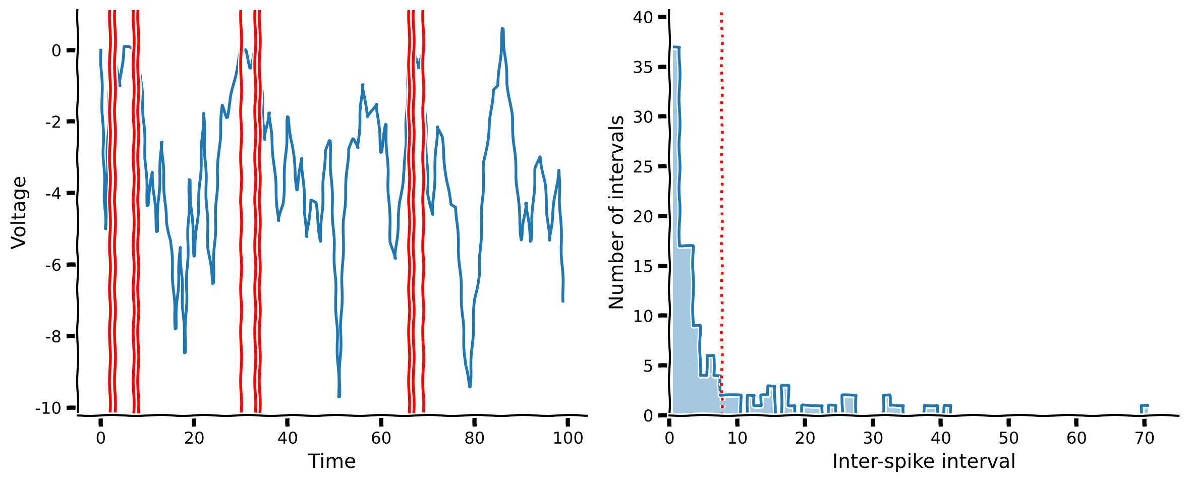
前節の線形積分発火ニューロンは確かにスパイクを生成できました。しかし、ISIヒストグラムはチュートリアル1で見た指数関数的な形状の実測ISIヒストグラムとはあまり似ていません。実際のニューロンのように振る舞わない理由は何でしょうか?
前のモデルでは興奮性の振る舞いのみを考慮しており、膜電位が減少するのはスパイクイベント時のみでした。しかし、膜電位を下げる他の要因もあります。まずニューロンは自然に安定状態や静止電位に戻ろうとする傾向があります。これを考慮してモデルを次のように更新できます:
ここで は現在の膜電位、 は漏れ係数です。これは人気のあるリーキー積分発火(LIF)モデルの基本形です(LIFニューロンの詳細な議論はボーナスセクション2や本コースの生物学的ニューロンモデルの日を参照してください)。
また、興奮性のシナプス前ニューロンに加えて抑制性のシナプス前ニューロンも存在します。これらの抑制性ニューロンは別のポアソン乱数でモデル化できます:
\begin{align}
I &= I_{\mathrm{exc}} - I_{\mathrm{inh}} \
I_{\mathrm{exc}} & \
I_{\mathrm{inh}} &\sim \mathrm{Poisson}(\lambda_{\mathrm{inh}})
\end{align}
ここで と はそれぞれ興奮性および抑制性シナプス前ニューロンの平均スパイク率(1タイムステップあたり)です。
コーディング演習 2: 抑制信号を含む の計算
2 回目の演習では、上で説明した LIF モデルニューロンの電圧変化 を計算するコードを書きます。前回同様、ニューロンダイナミクスを扱うための残りのコードは用意されているので、以下の dv の定義だけを埋めればよいです。
def lif_neuron_inh(n_steps=1000, alpha=0.5, beta=0.1, exc_rate=10, inh_rate=10):
  """ Simulate a simplified leaky integrate-and-fire neuron with both excitatory
  and inhibitory inputs.

  Args:
    n_steps (int): The number of time steps to simulate the neuron's activity.
    alpha (float): The input scaling factor
    beta (float): The membrane potential leakage factor
    exc_rate (int): The mean rate of the incoming excitatory spikes
    inh_rate (int): The mean rate of the incoming inhibitory spikes
  """

  # precompute Poisson samples for speed
  exc = stats.poisson(exc_rate).rvs(n_steps)
  inh = stats.poisson(inh_rate).rvs(n_steps)

  v = np.zeros(n_steps)
  spike_times = []

  ###############################################################################
  # Students: compute dv, then comment out or remove the next line
  raise NotImplementedError("Exercise: compute the change in membrane potential")
  ################################################################################

  for i in range(1, n_steps):

    dv = ...

    v[i] = v[i-1] + dv
    if v[i] > 1:
      spike_times.append(i)
      v[i] = 0

  return v, spike_times

# Set random seed (for reproducibility)
np.random.seed(12)

# Model LIF neuron
v, spike_times = lif_neuron_inh()

# Visualize
plot_neuron_stats(v, spike_times)出力例:
# @title Submit your feedback
content_review(f"{feedback_prefix}_Compute_dVm_with_inhibitory_signals_Exercise")
インタラクティブデモ 2: LIF + 抑制ニューロン
インタラクティブデモ 1 と同様に、LIF ニューロンへの入力パラメータを操作して、その挙動を可視化できます。ここでは、入力をスケールする alpha に加え、電圧の漏れ係数である beta、興奮性の前シナプスニューロンの平均発火率 exc_rate、抑制性の前シナプスニューロンの平均発火率 inh_rate も調整できます。
- 興奮性発火率を上げるとどんな影響がありますか?
- 抑制性発火率を上げるとどんな影響がありますか?
- 興奮性と抑制性の両方の発火率を上げたらどうなりますか?
- ISI(発火間隔)の分布は、チュートリアル 1 で観察したデータのような形になりますか?
#@title
#@markdown **Run the cell** to enable the sliders.
def _lif_neuron_inh(n_steps=1000, alpha=0.5, beta=0.1, exc_rate=10, inh_rate=10):
  """ Simulate a simplified leaky integrate-and-fire neuron with both excitatory
  and inhibitory inputs.

  Args:
    n_steps (int): The number of time steps to simulate the neuron's activity.
    alpha (float): The input scaling factor
    beta (float): The membrane potential leakage factor
    exc_rate (int): The mean rate of the incoming excitatory spikes
    inh_rate (int): The mean rate of the incoming inhibitory spikes
  """
  # precompute Poisson samples for speed
  exc = stats.poisson(exc_rate).rvs(n_steps)
  inh = stats.poisson(inh_rate).rvs(n_steps)

  v = np.zeros(n_steps)
  spike_times = []
  for i in range(1, n_steps):
    dv = -beta * v[i-1] + alpha * (exc[i] - inh[i])
    v[i] = v[i-1] + dv
    if v[i] > 1:
      spike_times.append(i)
      v[i] = 0

  return v, spike_times

@widgets.interact(alpha=widgets.FloatLogSlider(0.5, min=-1, max=1),
                  beta=widgets.FloatLogSlider(0.1, min=-1, max=0),
                  exc_rate=widgets.IntSlider(12, min=10, max=20),
                  inh_rate=widgets.IntSlider(12, min=10, max=20))
def plot_lif_neuron(alpha=0.5, beta=0.1, exc_rate=10, inh_rate=10):
  v, spike_times = _lif_neuron_inh(2000, alpha, beta, exc_rate, inh_rate)
plot_neuron_stats(v, spike_times)# @title Submit your feedback
content_review(f"{feedback_prefix}_LIF_and_inhibition_neuron_Interactive_Demo_and_Discussion")# @title Video 3: LIF + inhibition
from ipywidgets import widgets
from IPython.display import YouTubeVideo
from IPython.display import IFrame
from IPython.display import display
class PlayVideo(IFrame):
def __init__(self, id, source, page=1, width=400, height=300, **kwargs):
self.id = id
if source == 'Bilibili':
src = f'https://player.bilibili.com/player.html?bvid={id}&page={page}'
elif source == 'Osf':
src = f'https://mfr.ca-1.osf.io/render?url=https://osf.io/download/{id}/?direct%26mode=render'
super(PlayVideo, self).__init__(src, width, height, **kwargs)
def display_videos(video_ids, W=400, H=300, fs=1):
tab_contents = []
for i, video_id in enumerate(video_ids):
out = widgets.Output()
with out:
if video_ids[i][0] == 'Youtube':
video = YouTubeVideo(id=video_ids[i][1], width=W,
height=H, fs=fs, rel=0)
print(f'Video available at https://youtube.com/watch?v={video.id}')
else:
video = PlayVideo(id=video_ids[i][1], source=video_ids[i][0], width=W,
height=H, fs=fs, autoplay=False)
if video_ids[i][0] == 'Bilibili':
print(f'Video available at https://www.bilibili.com/video/{video.id}')
elif video_ids[i][0] == 'Osf':
print(f'Video available at https://osf.io/{video.id}')
display(video)
tab_contents.append(out)
return tab_contents
video_ids = [('Youtube', 'Aq7JrxRkn2w'), ('Bilibili', 'BV1nV41167mS')]
tab_contents = display_videos(video_ids, W=854, H=480)
tabs = widgets.Tab()
tabs.children = tab_contents
for i in range(len(tab_contents)):
tabs.set_title(i, video_ids[i][0])
display(tabs)# @title Submit your feedback
content_review(f"{feedback_prefix}_LIF_and_inhibition_Video")セクション 3: モデルのあり方を振り返る
チュートリアル開始からここまでの推定所要時間: 35 分
考えよう!3: モデルのあり方を振り返る
以下の質問について、グループで約 10 分間話し合ってください:
- これまでに「モデルのあり方」を見たことがありますか?
- 自分で作ったことはありますか?
- なぜ「モデルのあり方」は役に立つのでしょう?
- いつ可能なのでしょう?あなたの分野には「モデルのあり方」がありますか?
- 作ることで何を学べますか?
# @title Submit your feedback
content_review(f"{feedback_prefix}_Reflecting_on_how_models_Discussion")
概要
チュートリアルの推定所要時間:45分
このチュートリアルでは、実際の神経データで観察される挙動を生み出すメカニズムについて直感を得ました。まず、興奮性入力を持つ単純なニューロンモデルを構築し、その挙動をISI分布を用いて測定しましたが、実際のニューロンとは一致しませんでした。次に、漏れ電流と抑制性入力を追加してモデルを改良しました。このバランスの取れたモデルの挙動は、実際の神経データにかなり近づきました。
記号の説明
\begin{align}
& \
d &\
&\
I &\
&\
V_ &\
&\
&\
&\
&\
&\
\end{align}
ボーナス
ボーナスセクション1:なぜニューロンは発火するのか?
ニューロンは細胞膜を挟んだ電場にエネルギーを蓄えています。これは膜の両側にある電荷(イオン)の分布を制御することで実現されます。このエネルギーは、膜電位(または電場電位)が閾値を超えたときに急速に放出され、スパイクを発生させます。膜電位は他のニューロンからの入力によって閾値に向かって動いたり、離れたりします。これらの入力はそれぞれ興奮性または抑制性です。膜電位はイオンの漏れなどにより静止電位に戻ろうとする傾向があるため、スパイク閾値に達するかどうかは、最後のスパイク以降に受けた入力の量だけでなく、その入力のタイミングにも依存します。
絶縁膜を挟んだ電場電位を維持してエネルギーを蓄えることはコンデンサでモデル化できます。膜を通じた電荷の漏れは抵抗でモデル化できます。これがリーキーインテグレート・アンド・ファイア(LIF)ニューロンモデルの基礎です。
ボーナスセクション2:LIFモデルニューロン
LIFニューロンの完全な方程式は次の通りです。
ここで、は膜容量、は膜抵抗、は静止電位、は入力電流(他のニューロンや電極などからのもの)です。
上記の例では、モデルの一般的な挙動に焦点を当てるために多くのパラメータを便利な値に設定しました(, )。しかし、これらのパラメータも異なる動的挙動を実現したり、シミュレーション単位と実験単位間で問題の次元を保つために調整可能です(例えば、をミリボルト、をメガオーム、をミリ秒で表す場合など)。