チュートリアル 1: 「何を」モデル化するか

第1週、第1日目：モデルの種類

Neuromatch Academyによる

コンテンツ作成者： Matt Laporte、Byron Galbraith、Konrad Kording

コンテンツレビュアー： Dalin Guo、Aishwarya Balwani、Madineh Sarvestani、Maryam Vaziri-Pashkam、Michael Waskom、Ella Batty

制作編集者： Gagana B、Spiros Chavlis

Steinmetz et al. (2019) によるデータ共有に感謝します。ここではそのデータの一部を使用しています。

チュートリアルの目的

チュートリアルの推定所要時間：50分

これは神経データを理解するために使われるさまざまなタイプのモデルに関する3部構成のシリーズの第1回目です。このチュートリアルでは、データを記述するために使われる「何を」モデル（Whatモデル）を探ります。データの様子を理解するために、さまざまな方法で可視化します。その後、単純な数学モデルと比較します。具体的には以下を行います。

• 数百のニューロンのスパイク活動を含むデータセットを読み込み、その構造を理解する
• 集団全体のスパイク活動の特徴を可視化するプロットを作成する
• 単一ニューロンの「インタースパイク間隔」（ISI）の分布を計算する
• この分布の形状に関するいくつかの形式的モデルを検討し、それらを「手作業」でデータにフィットさせる

# @title Tutorial slides
# @markdown These are the slides for the videos in all tutorials today
from IPython.display import IFrame
link_id = "6dxwe"
print(f"If you want to download the slides: https://osf.io/download/{link_id}/")
IFrame(src=f"https://mfr.ca-1.osf.io/render?url=https://osf.io/{link_id}/?direct%26mode=render%26action=download%26mode=render", width=854, height=480)

セットアップ

# @title Install and import feedback gadget


from vibecheck import DatatopsContentReviewContainer
def content_review(notebook_section: str):
    return DatatopsContentReviewContainer(
        "",  # No text prompt
        notebook_section,
        {
            "url": "https://pmyvdlilci.execute-api.us-east-1.amazonaws.com/klab",
            "name": "neuromatch_cn",
            "user_key": "y1x3mpx5",
        },
    ).render()


feedback_prefix = "W1D1_T1"

Pythonでは、ライブラリの関数を使う前に明示的に「import」する必要があります。ノートブックやスクリプトの冒頭で必ずインポートを指定します。

import numpy as np
import matplotlib.pyplot as plt

チュートリアルノートブックは通常、最初にいくつかのセットアップ手順があり、デフォルトでは非表示になっています。

重要： コードが隠れていても、ノートブックの他の部分が正しく動作するために必ず実行してください。左上の再生ボタンを押すか、キーボードショートカット（MacではCmd-Return、それ以外はCtrl-Enter）で各セルを順に実行します。実行されると、ブラケット内に番号（例：[3]）が表示され、実行順序がわかります。

各セルの中身を見たい場合は、ダブルクリックで展開できます。展開後は、エディタ右側の白いスペースをダブルクリックすると再び折りたたむことができます。

# @title Figure Settings
import logging
logging.getLogger('matplotlib.font_manager').disabled = True

import ipywidgets as widgets  # interactive display
%matplotlib inline
%config InlineBackend.figure_format = 'retina'
plt.style.use("https://raw.githubusercontent.com/NeuromatchAcademy/course-content/main/nma.mplstyle")

# @title Plotting functions

def plot_isis(single_neuron_isis):
  plt.hist(single_neuron_isis, bins=50, histtype="stepfilled")
  plt.axvline(single_neuron_isis.mean(), color="orange", label="Mean ISI")
  plt.xlabel("ISI duration (s)")
  plt.ylabel("Number of spikes")
  plt.legend()

#@title Data retrieval
#@markdown This cell downloads the example dataset that we will use in this tutorial.
import io
import requests
r = requests.get('https://osf.io/sy5xt/download')
if r.status_code != 200:
  print('Failed to download data')
else:
  spike_times = np.load(io.BytesIO(r.content), allow_pickle=True)['spike_times']

「What」モデル

# @title Video 1: "What" Models
from ipywidgets import widgets
from IPython.display import YouTubeVideo
from IPython.display import IFrame
from IPython.display import display


class PlayVideo(IFrame):
  def __init__(self, id, source, page=1, width=400, height=300, **kwargs):
    self.id = id
    if source == 'Bilibili':
      src = f'https://player.bilibili.com/player.html?bvid={id}&page={page}'
    elif source == 'Osf':
      src = f'https://mfr.ca-1.osf.io/render?url=https://osf.io/download/{id}/?direct%26mode=render'
    super(PlayVideo, self).__init__(src, width, height, **kwargs)


def display_videos(video_ids, W=400, H=300, fs=1):
  tab_contents = []
  for i, video_id in enumerate(video_ids):
    out = widgets.Output()
    with out:
      if video_ids[i][0] == 'Youtube':
        video = YouTubeVideo(id=video_ids[i][1], width=W,
                             height=H, fs=fs, rel=0)
        print(f'Video available at https://youtube.com/watch?v={video.id}')
      else:
        video = PlayVideo(id=video_ids[i][1], source=video_ids[i][0], width=W,
                          height=H, fs=fs, autoplay=False)
        if video_ids[i][0] == 'Bilibili':
          print(f'Video available at https://www.bilibili.com/video/{video.id}')
        elif video_ids[i][0] == 'Osf':
          print(f'Video available at https://osf.io/{video.id}')
      display(video)
    tab_contents.append(out)
  return tab_contents


video_ids = [('Youtube', 'KgqR_jbjMQg'), ('Bilibili', 'BV1mz4y1X7ot')]
tab_contents = display_videos(video_ids, W=854, H=480)
tabs = widgets.Tab()
tabs.children = tab_contents
for i in range(len(tab_contents)):
  tabs.set_title(i, video_ids[i][0])
display(tabs)

# @title Submit your feedback
content_review(f"{feedback_prefix}_What_models_Video")

セクション 1: Steinmetz データセットの探索

このチュートリアルでは、神経科学のデータセットの構造を探索します。

ここでは、Steinmetz et al. (2019) の研究からのデータの一部を扱います。この研究では、Neuropixels プローブがマウスの脳に埋め込まれました。各プローブの長さに沿って数百の電極で電位が測定されました。各電極の測定は、近くのスパイクするニューロンによる電場の局所的な変動を捉えています。スパイクソーティングアルゴリズムを用いてスパイク時刻を推定し、共通の起源に基づいてスパイクをクラスタリングしました：ソートされたスパイクの単一クラスタは、因果的に単一のニューロンに帰属されます。

特に、スパイク時刻とニューロン割り当ての単一の記録セッションが読み込まれ、前のセットアップで spike_times に割り当てられています。

通常、データセットにはその構造に関する情報が付属しています。しかし、この情報は不完全な場合があります。また、関心のあるデータの作業用表現を作成するために、いくつかの変換や「前処理」を適用することもあり、その過程が部分的に文書化されていないこともあります。いずれにせよ、利用可能なツールを使って未知のデータ構造の側面を調査できることが重要です。

それでは、私たちのデータがどのようなものか見てみましょう...

セクション 1.1: spike_times でウォーミングアップ

変数のPythonの型は何でしょうか？

type(spike_times)

numpy.ndarray と表示されるはずです。これは通常のNumPy配列であることを意味します。

エラーメッセージが表示される場合は、おそらくノートブックの最初のセットアップセルを実行していないことが原因です。なので、必ず実行してください。

すべてが正常に動作していることを確認したら、次の質問をしましょう：データセットの形状はどうなっていますか？

spike_times.shape

1次元に734個のエントリがあり、他の次元はありません。最初のエントリのPythonの型は何で、その形状はどうなっていますか？

idx = 0
print(
  type(spike_times[idx]),
  spike_times[idx].shape,
  sep="\n",
)

これも1次元の形状を持つNumPy配列です！なぜこれがspike_timesの形状において第2の次元として現れなかったのでしょうか？つまり、なぜspike_times.shape == (734, 826)ではないのでしょう？

調査のために、別のエントリを確認してみましょう。

idx = 321
print(
  type(spike_times[idx]),
  spike_times[idx].shape,
  sep="\n",
)

これも1次元のNumPy配列ですが、形状が異なります。これらの配列の値のNumPy型と最初の数個の要素を確認すると、浮動小数点数（別のレベルのnp.ndarrayではありません）で構成されていることがわかります：

i_neurons = [0, 321]
i_print = slice(0, 5)

for i in i_neurons:
  print(
    "Neuron {}:".format(i),
    spike_times[i].dtype,
    spike_times[i][i_print],
    "\n",
    sep="\n"
  )

今回はPythonの変数型ではなくNumPyのdtypeを確認したことに注意してください。これら2つの配列は32ビット精度の浮動小数点数（「float」）を含んでいます。

基本的なイメージは次のようになります：

• spike_timesは1次元で、そのエントリはNumPy配列であり、その長さはニューロンの数（734）です：インデックスを指定することでニューロンのサブセットを選択します。
• spike_timesの中の配列も1次元で、単一のニューロンに対応し、そのエントリは浮動小数点数で、その長さはそのニューロンに割り当てられたスパイクの数です。インデックスを指定することで、そのニューロンのスパイク時刻のサブセットを選択します。

視覚的には、データ構造は次のように見えると考えられます：

| . . . . . |
| . . . . . . . . |
| . . . |
| . . . . . . . |

先に進む前に、データセット内のニューロンの数とニューロンごとのスパイク数を計算して保存しましょう。

n_neurons = len(spike_times)
total_spikes_per_neuron = [len(spike_times_i) for spike_times_i in spike_times]

print(f"Number of neurons: {n_neurons}")
print(f"Number of spikes for first five neurons: {total_spikes_per_neuron[:5]}")

# @title Video 2: Exploring the dataset
from ipywidgets import widgets
from IPython.display import YouTubeVideo
from IPython.display import IFrame
from IPython.display import display


class PlayVideo(IFrame):
  def __init__(self, id, source, page=1, width=400, height=300, **kwargs):
    self.id = id
    if source == 'Bilibili':
      src = f'https://player.bilibili.com/player.html?bvid={id}&page={page}'
    elif source == 'Osf':
      src = f'https://mfr.ca-1.osf.io/render?url=https://osf.io/download/{id}/?direct%26mode=render'
    super(PlayVideo, self).__init__(src, width, height, **kwargs)


def display_videos(video_ids, W=400, H=300, fs=1):
  tab_contents = []
  for i, video_id in enumerate(video_ids):
    out = widgets.Output()
    with out:
      if video_ids[i][0] == 'Youtube':
        video = YouTubeVideo(id=video_ids[i][1], width=W,
                             height=H, fs=fs, rel=0)
        print(f'Video available at https://youtube.com/watch?v={video.id}')
      else:
        video = PlayVideo(id=video_ids[i][1], source=video_ids[i][0], width=W,
                          height=H, fs=fs, autoplay=False)
        if video_ids[i][0] == 'Bilibili':
          print(f'Video available at https://www.bilibili.com/video/{video.id}')
        elif video_ids[i][0] == 'Osf':
          print(f'Video available at https://osf.io/{video.id}')
      display(video)
    tab_contents.append(out)
  return tab_contents


video_ids = [('Youtube', 'oHwYWUI_o1U'), ('Bilibili', 'BV1Hp4y1S7Au')]
tab_contents = display_videos(video_ids, W=854, H=480)
tabs = widgets.Tab()
tabs.children = tab_contents
for i in range(len(tab_contents)):
  tabs.set_title(i, video_ids[i][0])
display(tabs)

# @title Submit your feedback
content_review(f"{feedback_prefix}_Exploring_the_dataset_Video")

セクション1.2：温まってきた：総スパイク数のカウントとプロット

これまで見てきたように、全記録期間におけるスパイク数はニューロン間で変動します。より一般的には、ある期間において一部のニューロンは他よりも多くスパイクを発生させる傾向があります。データセット内の全ニューロンにわたるスパイクの分布を調べてみましょう。

ほとんどのニューロンは平均と比べて「うるさい」でしょうか、それとも「静か」でしょうか？これを見るために、総スパイク数の一定幅のビンを定義し、そのビンに入るニューロン数をカウントします。これは「ヒストグラム」として知られています。

matplotlibの関数plt.histでヒストグラムをプロットできます。計算だけが必要な場合は、numpyの関数np.histogramを使うこともできます。

plt.hist(total_spikes_per_neuron, bins=50, histtype="stepfilled")
plt.xlabel("Total spikes per neuron")
plt.ylabel("Number of neurons");

平均以下のスパイク数を持つニューロンの割合を見てみましょう：

mean_spike_count = np.mean(total_spikes_per_neuron)
frac_below_mean = (total_spikes_per_neuron < mean_spike_count).mean()
print(f"{frac_below_mean:2.1%} of neurons are below the mean")

平均スパイク数をヒストグラムのプロットに追加してもこれがわかります：

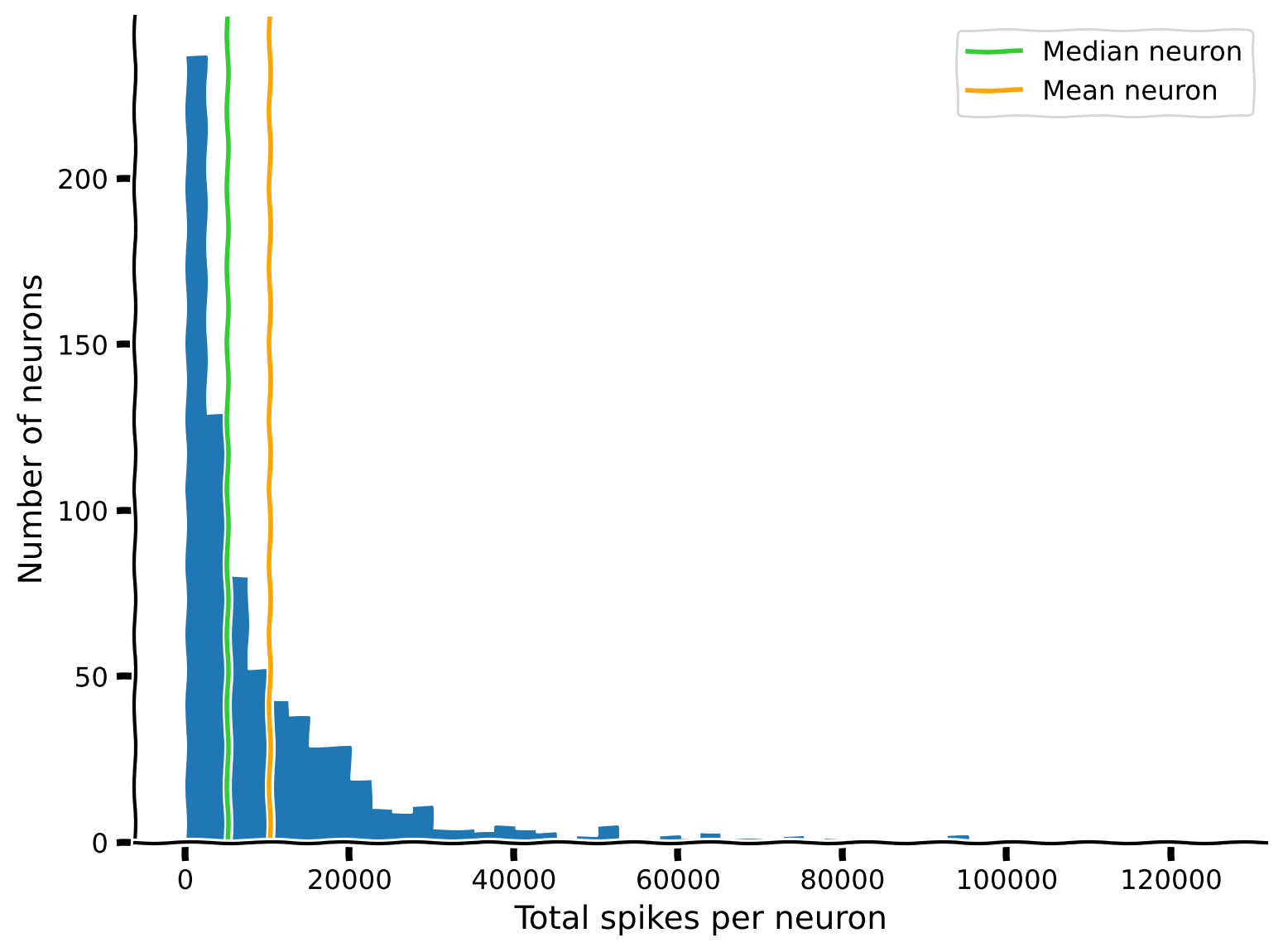
plt.hist(total_spikes_per_neuron, bins=50, histtype="stepfilled")
plt.xlabel("Total spikes per neuron")
plt.ylabel("Number of neurons")
plt.axvline(mean_spike_count, color="orange", label="Mean neuron")
plt.legend();

これは、ほとんどのニューロンが平均と比べて比較的「静か」であり、一部のニューロンは非常に「うるさい」ことを示しています：大きなスパイク数に達するためにより頻繁にスパイクしているに違いありません。

コーディング演習1.2：平均ニューロンと中央値ニューロンの比較

もし平均ニューロンが集団の68％よりも活発であるならば、それは平均ニューロンと中央値ニューロンの関係について何を意味するでしょうか？

演習の目的: 上記のプロットを再現し、中央値ニューロンを追加してください。

#################################################################################
## TODO for students:
# Fill out function and remove
raise NotImplementedError("Student exercise: complete histogram plotting with median")
#################################################################################

# Compute median spike count
median_spike_count = ...  # Hint: Try the function np.median

# Visualize median, mean, and histogram
plt.hist(..., bins=50, histtype="stepfilled")
plt.axvline(..., color="limegreen", label="Median neuron")
plt.axvline(mean_spike_count, color="orange", label="Mean neuron")
plt.xlabel("Total spikes per neuron")
plt.ylabel("Number of neurons")
plt.legend()

解答を見る$

出力例:

ボーナス: 中央値は50パーセンタイルです。他のパーセンタイルはどうでしょうか？ヒストグラムに四分位範囲を表示できますか？

# @title Submit your feedback
content_review(f"{feedback_prefix}_Comparing_mean_and_median_neurons_Exercise")

セクション 2: ニューロンのスパイク活動の可視化

チュートリアル開始からここまでの推定時間: 15分

セクション 2.1: データのサブセット取得

これからスパイク列を可視化します。記録が長いため、まず短い時間間隔を定義し、この間隔内のスパイクのみを可視化対象に制限します。これを行うためのヘルパー関数 restrict_spike_times を用意しました。この関数に対して help() を呼び出すと、関数の簡単な説明が表示されます。

# @markdown Execute this cell for helper function `restrict_spike_times`
def restrict_spike_times(spike_times, interval):
  """Given a spike_time dataset, restrict to spikes within given interval.

  Args:
    spike_times (sequence of np.ndarray): List or array of arrays,
      each inner array has spike times for a single neuron.
    interval (tuple): Min, max time values; keep min <= t < max.

  Returns:
    np.ndarray: like `spike_times`, but only within `interval`
  """
  interval_spike_times = []
  for spikes in spike_times:
    interval_mask = (spikes >= interval[0]) & (spikes < interval[1])
    interval_spike_times.append(spikes[interval_mask])
  return np.array(interval_spike_times, object)

help(restrict_spike_times)

t_interval = (5, 15)  # units are seconds after start of recording
interval_spike_times = restrict_spike_times(spike_times, t_interval)

この間隔は代表的なものですか？全スパイクのうちこの間隔に含まれる割合はどれくらいですか？

original_counts = sum([len(spikes) for spikes in spike_times])
interval_counts = sum([len(spikes) for spikes in interval_spike_times])
frac_interval_spikes = interval_counts / original_counts
print(f"{frac_interval_spikes:.2%} of the total spikes are in the interval")

この割合は、間隔の長さと実験全体の長さの比率とどう比較されますか？（全時間のうちこの間隔が占める割合は？）

実験の全期間は、全データセットのスパイク時刻の最小値と最大値を取ることで近似できます。そのために、すべてのニューロンのスパイク時刻を一つの配列に「連結」し、np.ptp（ピーク・トゥ・ピーク）を使って最大値と最小値の差を取得します。

spike_times_flat = np.concatenate(spike_times)
experiment_duration = np.ptp(spike_times_flat)
interval_duration = t_interval[1] - t_interval[0]

frac_interval_time = interval_duration / experiment_duration
print(f"{frac_interval_time:.2%} of the total time is in the interval")

これら2つの値、すなわち全スパイクに占める割合と全時間に占める割合は似ています。これは、この間隔内のニューロン集団の平均スパイク率が全記録期間と比較して大きく異ならないことを示唆しています。

セクション 2.2: スパイク列とラスターのプロット

代表的なサブセットが得られたので、matplotlib の plt.eventplot 関数を使ってスパイクをプロットしましょう。まずは単一のニューロンを見てみます。

neuron_idx = 1
plt.eventplot(interval_spike_times[neuron_idx], color=".2")
plt.xlabel("Time (s)")
plt.yticks([]);

複数のニューロンもプロットできます。ここでは3つのニューロンを示します。

neuron_idx = [1, 11, 51]
plt.eventplot(interval_spike_times[neuron_idx], color=".2")
plt.xlabel("Time (s)")
plt.yticks([]);

これは「ラスター」プロットを作成し、各ニューロンのスパイクが異なる行に表示されます。

多数のニューロンをプロットすると、集団の特徴を把握できます。記録されたニューロンのうち5つおきに表示してみましょう。

neuron_idx = np.arange(0, len(spike_times), 5)
plt.eventplot(interval_spike_times[neuron_idx], color=".2")
plt.xlabel("Time (s)")
plt.yticks([]);

質問: このプロットの情報は、上で見た総スパイク数のヒストグラムとどのように関連していますか？

解答を見る$

# @title Video 3: Visualizing activity
from ipywidgets import widgets
from IPython.display import YouTubeVideo
from IPython.display import IFrame
from IPython.display import display


class PlayVideo(IFrame):
  def __init__(self, id, source, page=1, width=400, height=300, **kwargs):
    self.id = id
    if source == 'Bilibili':
      src = f'https://player.bilibili.com/player.html?bvid={id}&page={page}'
    elif source == 'Osf':
      src = f'https://mfr.ca-1.osf.io/render?url=https://osf.io/download/{id}/?direct%26mode=render'
    super(PlayVideo, self).__init__(src, width, height, **kwargs)


def display_videos(video_ids, W=400, H=300, fs=1):
  tab_contents = []
  for i, video_id in enumerate(video_ids):
    out = widgets.Output()
    with out:
      if video_ids[i][0] == 'Youtube':
        video = YouTubeVideo(id=video_ids[i][1], width=W,
                             height=H, fs=fs, rel=0)
        print(f'Video available at https://youtube.com/watch?v={video.id}')
      else:
        video = PlayVideo(id=video_ids[i][1], source=video_ids[i][0], width=W,
                          height=H, fs=fs, autoplay=False)
        if video_ids[i][0] == 'Bilibili':
          print(f'Video available at https://www.bilibili.com/video/{video.id}')
        elif video_ids[i][0] == 'Osf':
          print(f'Video available at https://osf.io/{video.id}')
      display(video)
    tab_contents.append(out)
  return tab_contents


video_ids = [('Youtube', 'QGA5FCW7kkA'), ('Bilibili', 'BV1dt4y1Q7C5')]
tab_contents = display_videos(video_ids, W=854, H=480)
tabs = widgets.Tab()
tabs.children = tab_contents
for i in range(len(tab_contents)):
  tabs.set_title(i, video_ids[i][0])
display(tabs)

# @title Submit your feedback
content_review(f"{feedback_prefix}_Visualizing_activity_Video")

セクション 3: スパイク間隔とその分布

チュートリアル開始からここまでの推定時間: 25分

spike_times にある各ニューロンの順序付けられたスパイク時刻配列を可視化しましたが、次に何を問うことができるでしょうか？

科学的な問いは既存のモデルに基づいています。では、このデータに関する問いを導くために、どんな知識を既に持っているでしょうか？

ニューロンのスパイクには物理的制約があることがわかっています。スパイクにはエネルギーが必要で、ニューロンの細胞機構は有限の速度でしかエネルギーを供給できません。したがって、ニューロンには不応期があり、代謝プロセスが支える速度でしか発火できず、同じニューロンの連続スパイク間には最小遅延があります。

より一般的には、「ニューロンは次のスパイクまでどれくらい待つのか？」「最長でどれくらい待つのか？」といった問いが考えられます。スパイク時刻を何か別のものに変換して、こうした問いにより直接的に答えられるでしょうか？

スパイク間隔（Inter-Spike Intervals: ISI）を考えられます。これは単に同じニューロンの連続スパイク間の時間差です。

演習 3: 単一ニューロンの ISI 分布をプロットしよう

演習の目的: スパイク数のヒストグラムと同様に、データセットの一つのニューロンの ISI 分布を示すヒストグラムを作成します。

3つのステップで行います：

1. あるニューロンのスパイク時刻を抽出する
2. ISI（スパイク間の時間、すなわち隣接するスパイク時刻の差）を計算する
3. 個々の ISI 配列でヒストグラムをプロットする

def compute_single_neuron_isis(spike_times, neuron_idx):
  """Compute a vector of ISIs for a single neuron given spike times.

  Args:
    spike_times (list of 1D arrays): Spike time dataset, with the first
      dimension corresponding to different neurons.
    neuron_idx (int): Index of the unit to compute ISIs for.

  Returns:
    isis (1D array): Duration of time between each spike from one neuron.
  """
  #############################################################################
  # Students: Fill in missing code (...) and comment or remove the next line
  raise NotImplementedError("Exercise: compute single neuron ISIs")
  #############################################################################

  # Extract the spike times for the specified neuron
  single_neuron_spikes = ...

  # Compute the ISIs for this set of spikes
  # Hint: the function np.diff computes discrete differences along an array
  isis = ...

  return isis

# Compute ISIs
single_neuron_isis = compute_single_neuron_isis(spike_times, neuron_idx=283)

# Visualize ISIs
plot_isis(single_neuron_isis)

解答を見る$

例の出力:

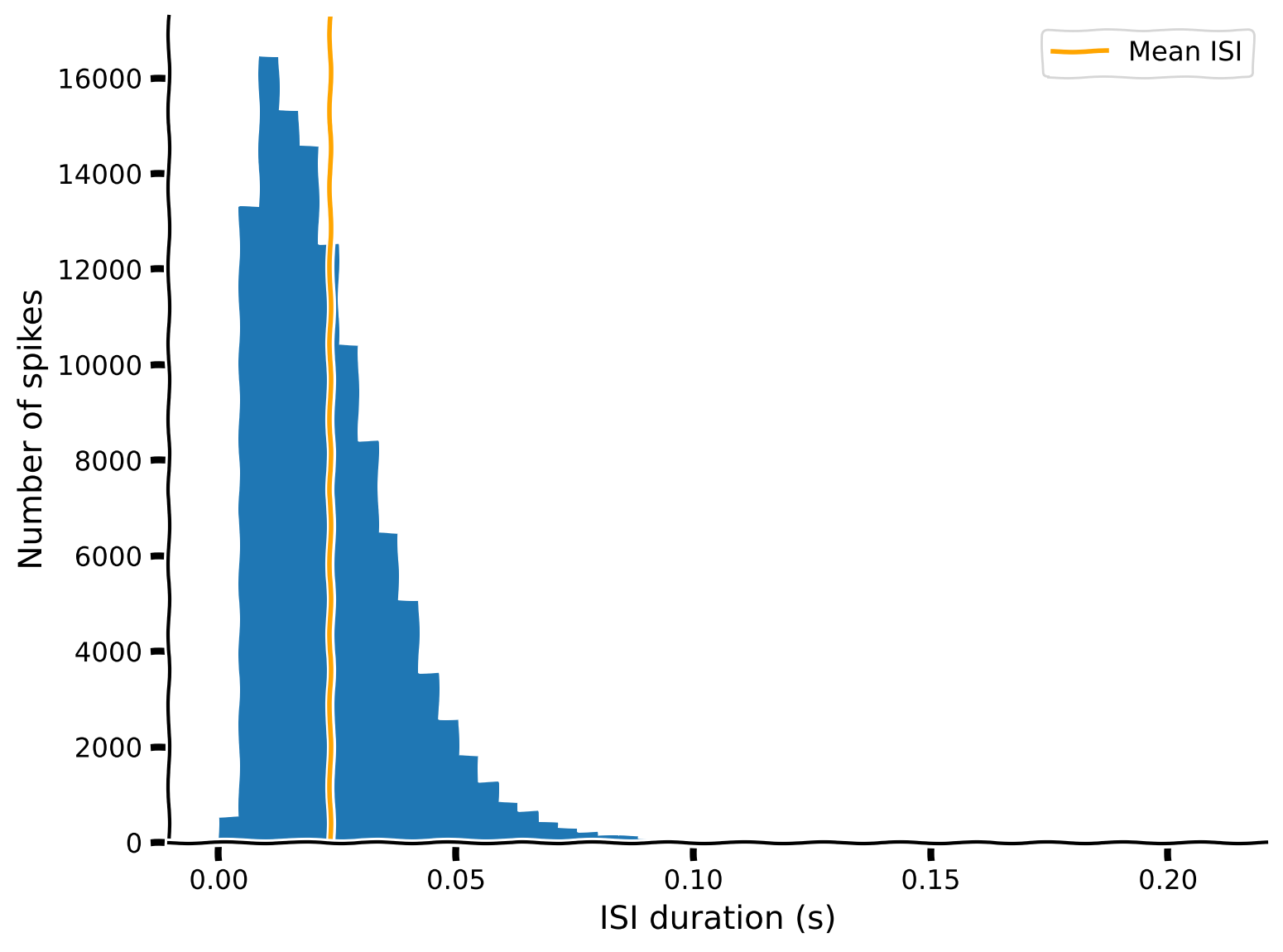
一般的に、短い ISI が優勢で、ISI が長くなるにつれてカウントは急速に（そしておおむね滑らかに）減少します。しかし、分布の最大値（8～11 ms）より短い ISI ではカウントが急速にゼロに近づきます。この非常に短い ISI の欠如は不応期仮説と一致し、ニューロンはこの領域の ISI 分布を埋めるほど速く発火できないことを示しています。

他のニューロンの分布も確認してみてください。分布のさまざまな特徴を解像するために、plt.hist の bins の値を調整する必要があるかもしれません。ビン数が少なすぎると興味深い詳細が平滑化されますが、多すぎるとランダムな変動が目立ってしまいます。

また、比較的短いまたは長い ISI に注目して分布の形状を見るために範囲を制限したい場合もあるでしょう。ヒント: plt.hist は range 引数を取ります。

# @title Submit your feedback
content_review(f"{feedback_prefix}_ISIs_and_their_distributions_Exercise")

セクション 4: ISI 分布の関数形は？

チュートリアル開始からここまでの推定時間: 35分

# @title Video 4: ISI distribution
from ipywidgets import widgets
from IPython.display import YouTubeVideo
from IPython.display import IFrame
from IPython.display import display


class PlayVideo(IFrame):
  def __init__(self, id, source, page=1, width=400, height=300, **kwargs):
    self.id = id
    if source == 'Bilibili':
      src = f'https://player.bilibili.com/player.html?bvid={id}&page={page}'
    elif source == 'Osf':
      src = f'https://mfr.ca-1.osf.io/render?url=https://osf.io/download/{id}/?direct%26mode=render'
    super(PlayVideo, self).__init__(src, width, height, **kwargs)


def display_videos(video_ids, W=400, H=300, fs=1):
  tab_contents = []
  for i, video_id in enumerate(video_ids):
    out = widgets.Output()
    with out:
      if video_ids[i][0] == 'Youtube':
        video = YouTubeVideo(id=video_ids[i][1], width=W,
                             height=H, fs=fs, rel=0)
        print(f'Video available at https://youtube.com/watch?v={video.id}')
      else:
        video = PlayVideo(id=video_ids[i][1], source=video_ids[i][0], width=W,
                          height=H, fs=fs, autoplay=False)
        if video_ids[i][0] == 'Bilibili':
          print(f'Video available at https://www.bilibili.com/video/{video.id}')
        elif video_ids[i][0] == 'Osf':
          print(f'Video available at https://osf.io/{video.id}')
      display(video)
    tab_contents.append(out)
  return tab_contents


video_ids = [('Youtube', 'DHhM80MOTe8'), ('Bilibili', 'BV1ov411B7Pm')]
tab_contents = display_videos(video_ids, W=854, H=480)
tabs = widgets.Tab()
tabs.children = tab_contents
for i in range(len(tab_contents)):
  tabs.set_title(i, video_ids[i][0])
display(tabs)

# @title Submit your feedback
content_review(f"{feedback_prefix}_ISI_distribution_Video")

ISI ヒストグラムは最大値を超えて連続的かつ単調減少する関数に従うように見えます。関数は明らかに非線形です。これらは単一の関数族に属すると考えられるでしょうか？

生理学的現象を説明するために数学的関数を使う考えを動機付けるために、指数関数、逆関数、線形関数といういくつかの異なる関数形を定義してみましょう。

def exponential(xs, scale, rate, x0):
  """A simple parameterized exponential function, applied element-wise.

  Args:
    xs (np.ndarray or float): Input(s) to the function.
    scale (float): Linear scaling factor.
    rate (float): Exponential growth (positive) or decay (negative) rate.
    x0 (float): Horizontal offset.

  """
  ys = scale * np.exp(rate * (xs - x0))
  return ys

def inverse(xs, scale, x0):
  """A simple parameterized inverse function (`1/x`), applied element-wise.

  Args:
    xs (np.ndarray or float): Input(s) to the function.
    scale (float): Linear scaling factor.
    x0 (float): Horizontal offset.

  """
  ys = scale / (xs - x0)
  return ys

def linear(xs, slope, y0):
  """A simple linear function, applied element-wise.

  Args:
    xs (np.ndarray or float): Input(s) to the function.
    slope (float): Slope of the line.
    y0 (float): y-intercept of the line.

  """
  ys = slope * xs + y0
  return ys

インタラクティブデモ 4: ISI 関数エクスプローラー

ここでは、これらの関数のパラメータを変化させて、結果の出力がデータにどれだけ合致するかを確認できるインタラクティブデモを用意しました。スライダーを動かしてパラメータを調整し、ヒストグラムの減少曲線にどれだけ近づけられるか試してみてください。これはデータに対してモデルをフィットさせる際に何をしようとしているかを体験するものです。

「インタラクティブデモ」セルには、スライダーで関数のパラメータを操作できるインターフェースを定義する隠しコードがあります。コードの動作は気にせず、セルを実行するだけでスライダーが有効になります。

• どのタイプの関数（指数関数／逆関数／線形関数）がデータに最もよく合いますか？

#@markdown Be sure to run this cell to enable the demo
# Don't worry about understanding this code! It's to setup an interactive plot.
single_neuron_idx = 283
single_neuron_spikes = spike_times[single_neuron_idx]
single_neuron_isis = np.diff(single_neuron_spikes)

counts, edges = np.histogram(
  single_neuron_isis,
  bins=50,
  range=(0, single_neuron_isis.max())
)

functions = dict(
  exponential=exponential,
  inverse=inverse,
  linear=linear,
)

colors = dict(
  exponential="C1",
  inverse="C2",
  linear="C4",
)

@widgets.interact(
  exp_scale=widgets.FloatSlider(1000, min=0, max=20000, step=250),
  exp_rate=widgets.FloatSlider(-10, min=-200, max=50, step=1),
  exp_x0=widgets.FloatSlider(0.1, min=-0.5, max=0.5, step=0.005),
  inv_scale=widgets.FloatSlider(1000, min=0, max=3e2, step=10),
  inv_x0=widgets.FloatSlider(0, min=-0.2, max=0.2, step=0.01),
  lin_slope=widgets.FloatSlider(-1e5, min=-6e5, max=1e5, step=10000),
  lin_y0=widgets.FloatSlider(10000, min=0, max=4e4, step=1000),
)
def fit_plot(
  exp_scale=1000, exp_rate=-10, exp_x0=0.1,
  inv_scale=1000, inv_x0=0,
  lin_slope=-1e5, lin_y0=2000,
):
  """Helper function for plotting function fits with interactive sliders."""
  func_params = dict(
    exponential=(exp_scale, exp_rate, exp_x0),
    inverse=(inv_scale, inv_x0),
    linear=(lin_slope, lin_y0),
  )
  f, ax = plt.subplots()
  ax.fill_between(edges[:-1], counts, step="post", alpha=.5)
  xs = np.linspace(1e-10, edges.max())
  for name, function in functions.items():
    ys = function(xs, *func_params[name])
    ax.plot(xs, ys, lw=3, color=colors[name], label=name);
  ax.set(
      xlim=(edges.min(), edges.max()),
      ylim=(0, counts.max() * 1.1),
      xlabel="ISI (s)",
      ylabel="Number of spikes",
  )
  ax.legend()
  plt.show()

解答を見る$

# @title Submit your feedback
content_review(f"{feedback_prefix}_ISI_functions_explorer_Interactive_Demo_and_Discussion")

# @title Video 5: Fitting models by hand
from ipywidgets import widgets
from IPython.display import YouTubeVideo
from IPython.display import IFrame
from IPython.display import display


class PlayVideo(IFrame):
  def __init__(self, id, source, page=1, width=400, height=300, **kwargs):
    self.id = id
    if source == 'Bilibili':
      src = f'https://player.bilibili.com/player.html?bvid={id}&page={page}'
    elif source == 'Osf':
      src = f'https://mfr.ca-1.osf.io/render?url=https://osf.io/download/{id}/?direct%26mode=render'
    super(PlayVideo, self).__init__(src, width, height, **kwargs)


def display_videos(video_ids, W=400, H=300, fs=1):
  tab_contents = []
  for i, video_id in enumerate(video_ids):
    out = widgets.Output()
    with out:
      if video_ids[i][0] == 'Youtube':
        video = YouTubeVideo(id=video_ids[i][1], width=W,
                             height=H, fs=fs, rel=0)
        print(f'Video available at https://youtube.com/watch?v={video.id}')
      else:
        video = PlayVideo(id=video_ids[i][1], source=video_ids[i][0], width=W,
                          height=H, fs=fs, autoplay=False)
        if video_ids[i][0] == 'Bilibili':
          print(f'Video available at https://www.bilibili.com/video/{video.id}')
        elif video_ids[i][0] == 'Osf':
          print(f'Video available at https://osf.io/{video.id}')
      display(video)
    tab_contents.append(out)
  return tab_contents


video_ids = [('Youtube', 'uW2HDk_4-wk'), ('Bilibili', 'BV1w54y1S7Eb')]
tab_contents = display_videos(video_ids, W=854, H=480)
tabs = widgets.Tab()
tabs.children = tab_contents
for i in range(len(tab_contents)):
  tabs.set_title(i, video_ids[i][0])
display(tabs)

# @title Submit your feedback
content_review(f"{feedback_prefix}_Fitting_models_by_hand_Video")

セクション 5: モデルについて振り返る

チュートリアル開始からここまでの推定時間: 40分

考えよう！5: モデルについて振り返る

以下の質問についてグループで約10分間話し合ってください：

• これまでにどんなモデルを見たことがありますか？
• モデルを作ったことはありますか？
• モデルはなぜ役立つのでしょうか？
• いつモデルは可能でしょうか？あなたの分野にはモデルがありますか？
• モデルを構築することで何を学べますか？

# @title Submit your feedback
content_review(f"{feedback_prefix}_Reflecting_on_what_models_Discussion")

まとめ

チュートリアルの推定所要時間: 50分

このチュートリアルでは、神経データを読み込み、データセットの構造を理解するために触ってみました。次に、(1) 集団全体の平均的な活動レベルと (2) 個々のニューロンの ISI 分布を可視化する基本的なプロットを作成しました。最後に、生理学的現象を理解・説明するために数学的形式主義を使うことを考え始めました。これらはすべて、データが「何であるか」を理解するための第一歩に過ぎません。

これは脳について何かを語れるモデルを開発するための最初のステップです。次の2つのチュートリアルではそこに焦点を当てます。