チュートリアル 1: オートエンコーダー入門

ボーナスデイ: オートエンコーダー

Neuromatch Academy 提供

コンテンツ作成者: Marco Brigham と CCNSS チーム (2014-2018)

コンテンツレビュアー: Itzel Olivos, Karen Schroeder, Karolina Stosio, Kshitij Dwivedi, Spiros Chavlis, Michael Waskom

制作編集: Spiros Chavlis

チュートリアルの目的

内部表現とオートエンコーダー

単純なアルゴリズムがどのようにしてデータの重要な側面を捉え、世界の堅牢なモデルを構築できるのでしょうか？

オートエンコーダーは、補助タスクを通じて内部表現を学習する人工ニューラルネットワーク（ANN）の一種です。つまり、実践による学習です。

主なタスクは、入力の圧縮表現に基づいて出力画像を再構成することです。このタスクは、入力に似た画像を生成しつつ、どの詳細を捨てるべきかをネットワークに教えます。

架空のMNIST認知タスクは、画像のノイズ除去、隠れた部分の推測、元の画像の向きの復元など、より複雑なタスクをまとめています。MNISTデータセットの手書き数字を使うのは、スパイクデータの時系列など他のタイプのデータよりも、類似画像や再構成の問題を識別しやすいためです。

MNIST認知タスク $

オートエンコーダーの魅力は、これらの内部表現を可視化できる点にあります。ボトルネック層は、入力層や出力層よりもユニット数が少ないことでデータ圧縮を強制します。さらに、この層を2つまたは3つのユニットに制限すると、オートエンコーダーがデータを2次元または3次元の潜在空間でどのように整理しているかを見ることができます。

ロードマップは以下の通りです：チュートリアル1（本チュートリアル）でオートエンコーダーの典型的な要素を学び、チュートリアル2で性能拡張方法を学び、チュートリアル3でMNIST認知タスクを解きます。

このチュートリアルでは以下を行います：

潜在空間の可視化に慣れ、*主成分分析（PCA）と非負値行列因子分解（NMF）*に適用する
単一隠れ層のANNオートエンコーダーを構築し訓練する
異なる次元の潜在空間を持つオートエンコーダーの表現力を検査する

セットアップ

# @title Install and import feedback gadget


from vibecheck import DatatopsContentReviewContainer
def content_review(notebook_section: str):
    return DatatopsContentReviewContainer(
        "",  # No text prompt
        notebook_section,
        {
            "url": "https://pmyvdlilci.execute-api.us-east-1.amazonaws.com/klab",
            "name": "neuromatch_cn",
            "user_key": "y1x3mpx5",
        },
    ).render()


feedback_prefix = "Bonus_Autoencoders_T1"

# Imports
import numpy as np
import matplotlib.pyplot as plt

import torch
from torch import nn, optim

from sklearn import decomposition
from sklearn.datasets import fetch_openml

# @title Figure settings
import logging
logging.getLogger('matplotlib.font_manager').disabled = True
%config InlineBackend.figure_format = 'retina'
plt.style.use("https://raw.githubusercontent.com/NeuromatchAcademy/course-content/NMA2020/nma.mplstyle")
fig_w, fig_h = plt.rcParams['figure.figsize']

# @title Helper functions


def downloadMNIST():
  """
  Download MNIST dataset and transform it to torch.Tensor

  Args:
    None

  Returns:
    x_train : training images (torch.Tensor) (60000, 28, 28)
    x_test  : test images (torch.Tensor) (10000, 28, 28)
    y_train : training labels (torch.Tensor) (60000, )
    y_train : test labels (torch.Tensor) (10000, )
  """
  X, y = fetch_openml('mnist_784', version=1, return_X_y=True, as_frame=False)
  # Trunk the data
  n_train = 60000
  n_test = 10000

  train_idx = np.arange(0, n_train)
  test_idx = np.arange(n_train, n_train + n_test)

  x_train, y_train = X[train_idx], y[train_idx]
  x_test, y_test = X[test_idx], y[test_idx]

  # Transform np.ndarrays to torch.Tensor
  x_train = torch.from_numpy(np.reshape(x_train,
                                        (len(x_train),
                                         28, 28)).astype(np.float32))
  x_test = torch.from_numpy(np.reshape(x_test,
                                       (len(x_test),
                                        28, 28)).astype(np.float32))

  y_train = torch.from_numpy(y_train.astype(int))
  y_test = torch.from_numpy(y_test.astype(int))

  return (x_train, y_train, x_test, y_test)


def init_weights_kaiming_uniform(layer):
  """
  Initializes weights from linear PyTorch layer
  with kaiming uniform distribution.

  Args:
    layer (torch.Module)
        Pytorch layer

  Returns:
    Nothing.
  """
  # check for linear PyTorch layer
  if isinstance(layer, nn.Linear):
    # initialize weights with kaiming uniform distribution
    nn.init.kaiming_uniform_(layer.weight.data)


def init_weights_kaiming_normal(layer):
  """
  Initializes weights from linear PyTorch layer
  with kaiming normal distribution.

  Args:
    layer (torch.Module)
        Pytorch layer

  Returns:
    Nothing.
  """
  # check for linear PyTorch layer
  if isinstance(layer, nn.Linear):
    # initialize weights with kaiming normal distribution
    nn.init.kaiming_normal_(layer.weight.data)


def get_layer_weights(layer):
  """
  Retrieves learnable parameters from PyTorch layer.

  Args:
    layer (torch.Module)
        Pytorch layer

  Returns:
    list with learnable parameters
  """
  # initialize output list
  weights = []

  # check whether layer has learnable parameters
  if layer.parameters():
    # copy numpy array representation of each set of learnable parameters
    for item in layer.parameters():
      weights.append(item.detach().numpy().copy())

  return weights


def eval_mse(y_pred, y_true):
  """
  Evaluates Mean Square Error (MSE) between y_pred and y_true

  Args:
    y_pred (torch.Tensor)
        prediction samples

    v (numpy array of floats)
        ground truth samples

  Returns:
    MSE(y_pred, y_true)
  """

  with torch.no_grad():
      criterion = nn.MSELoss()
      loss = criterion(y_pred, y_true)

  return float(loss)


def eval_bce(y_pred, y_true):
  """
  Evaluates Binary Cross-Entropy (BCE) between y_pred and y_true

  Args:
    y_pred (torch.Tensor)
        prediction samples

    v (numpy array of floats)
        ground truth samples

  Returns:
    BCE(y_pred, y_true)
  """

  with torch.no_grad():
      criterion = nn.BCELoss()
      loss = criterion(y_pred, y_true)

  return float(loss)


def plot_weights_ab(encoder_w_a, encoder_w_b, decoder_w_a, decoder_w_b,
                    label_a='init', label_b='train',
                    bins_encoder=0.5, bins_decoder=1.5):
  """
  Plots row of histograms with encoder and decoder weights
  between two training checkpoints.

  Args:
    encoder_w_a (iterable)
        encoder weights at checkpoint a

    encoder_w_b (iterable)
        encoder weights at checkpoint b

    decoder_w_a (iterable)
        decoder weights at checkpoint a

    decoder_w_b (iterable)
        decoder weights at checkpoint b

    label_a (string)
        label for checkpoint a

    label_b (string)
        label for checkpoint b

    bins_encoder (float)
        norm of extreme values for encoder bins

    bins_decoder (float)
        norm of extreme values for decoder bins

  Returns:
    Nothing.
  """

  plt.figure(figsize=(fig_w * 1.2, fig_h * 1.2))

  # plot encoder weights
  bins = np.linspace(-bins_encoder, bins_encoder, num=32)

  plt.subplot(221)
  plt.title('Encoder weights to unit 0')
  plt.hist(encoder_w_a[0].flatten(), bins=bins, alpha=0.3, label=label_a)
  plt.hist(encoder_w_b[0].flatten(), bins=bins, alpha=0.3, label=label_b)
  plt.legend()

  plt.subplot(222)
  plt.title('Encoder weights to unit 1')
  plt.hist(encoder_w_a[1].flatten(), bins=bins, alpha=0.3, label=label_a)
  plt.hist(encoder_w_b[1].flatten(), bins=bins, alpha=0.3, label=label_b)
  plt.legend()

  # plot decoder weights
  bins = np.linspace(-bins_decoder, bins_decoder, num=32)

  plt.subplot(223)
  plt.title('Decoder weights from unit 0')
  plt.hist(decoder_w_a[:, 0].flatten(), bins=bins, alpha=0.3, label=label_a)
  plt.hist(decoder_w_b[:, 0].flatten(), bins=bins, alpha=0.3, label=label_b)
  plt.legend()

  plt.subplot(224)
  plt.title('Decoder weights from unit 1')
  plt.hist(decoder_w_a[:, 1].flatten(), bins=bins, alpha=0.3, label=label_a)
  plt.hist(decoder_w_b[:, 1].flatten(), bins=bins, alpha=0.3, label=label_b)
  plt.legend()

  plt.tight_layout()
  plt.show()


def plot_row(images, show_n=10, image_shape=None):
  """
  Plots rows of images from list of iterables (iterables: list, numpy array
  or torch.Tensor). Also accepts single iterable.
  Randomly selects images in each list element if item count > show_n.

  Args:
    images (iterable or list of iterables)
        single iterable with images, or list of iterables

    show_n (integer)
        maximum number of images per row

    image_shape (tuple or list)
        original shape of image if vectorized form

  Returns:
    Nothing.
  """

  if not isinstance(images, (list, tuple)):
    images = [images]

  for items_idx, items in enumerate(images):

    items = np.array(items)
    if items.ndim == 1:
      items = np.expand_dims(items, axis=0)

    if len(items) > show_n:
      selected = np.random.choice(len(items), show_n, replace=False)
      items = items[selected]

    if image_shape is not None:
      items = items.reshape([-1] + list(image_shape))

    plt.figure(figsize=(len(items) * 1.5, 2))
    for image_idx, image in enumerate(items):

      plt.subplot(1, len(items), image_idx + 1)
      plt.imshow(image, cmap='gray', vmin=image.min(), vmax=image.max())
      plt.axis('off')

      plt.tight_layout()


def xy_lim(x):
  """
  Return arguments for plt.xlim and plt.ylim calculated from minimum
  and maximum of x.

  Args:
    x (list, numpy array or torch.Tensor of floats)
        data to be plotted

  Returns:
    Nothing.
  """

  x_min = np.min(x, axis=0)
  x_max = np.max(x, axis=0)

  x_min = x_min - np.abs(x_max - x_min) * 0.05 - np.finfo(float).eps
  x_max = x_max + np.abs(x_max - x_min) * 0.05 + np.finfo(float).eps

  return [x_min[0], x_max[0]], [x_min[1], x_max[1]]


def plot_generative(x, decoder_fn, image_shape, n_row=16):
  """
  Plots images reconstructed by decoder_fn from a 2D grid in
  latent space that is determined by minimum and maximum values in x.

  Args:
    x (list, numpy array or torch.Tensor of floats)
        2D coordinates in latent space

    decoder_fn (integer)
        function returning vectorized images from 2D latent space coordinates

    image_shape (tuple or list)
        original shape of image

    n_row
        number of rows in grid

  Returns:
    Nothing.
  """

  xlim, ylim = xy_lim(np.array(x))

  dx = (xlim[1] - xlim[0]) / n_row
  grid = [np.linspace(ylim[0] + dx / 2, ylim[1] - dx / 2, n_row),
          np.linspace(xlim[0] + dx / 2, xlim[1] - dx / 2, n_row)]

  canvas = np.zeros((image_shape[0]*n_row, image_shape[1] * n_row))

  cmap = plt.get_cmap('gray')

  for j, latent_y in enumerate(grid[0][::-1]):
    for i, latent_x in enumerate(grid[1]):

      latent = np.array([[latent_x, latent_y]], dtype=np.float32)
      with torch.no_grad():
          x_decoded = decoder_fn(torch.from_numpy(latent))

      x_decoded = x_decoded.reshape(image_shape)

      canvas[j*image_shape[0]: (j + 1) * image_shape[0],
             i*image_shape[1]: (i + 1) * image_shape[1]] = x_decoded

  plt.imshow(canvas, cmap=cmap, vmin=canvas.min(), vmax=canvas.max())
  plt.axis('off')


def plot_latent(x, y, show_n=500, fontdict=None, xy_labels=None):
  """
  Plots digit class of each sample in 2D latent space coordinates.

  Args:
    x (list, numpy array or torch.Tensor of floats)
        2D coordinates in latent space

    y (list, numpy array or torch.Tensor of floats)
        digit class of each sample

    n_row (integer)
        number of samples

    fontdict (dictionary)
        optional style option for plt.text

    xy_labels (list)
        optional list with [xlabel, ylabel]

  Returns:
    Nothing.
  """

  if fontdict is None:
    fontdict = {'weight': 'bold', 'size': 12}

  cmap = plt.get_cmap('tab10')

  if len(x) > show_n:
    selected = np.random.choice(len(x), show_n, replace=False)
    x = x[selected]
    y = y[selected]

  for my_x, my_y in zip(x, y):
    plt.text(my_x[0], my_x[1], str(int(my_y)),
             color=cmap(int(my_y) / 10.),
             fontdict=fontdict,
             horizontalalignment='center',
             verticalalignment='center',
             alpha=0.8)

  if xy_labels is None:
    xy_labels = ['$Z_1$', '$Z_2$']

  plt.xlabel(xy_labels[0])
  plt.ylabel(xy_labels[1])

  xlim, ylim = xy_lim(np.array(x))
  plt.xlim(xlim)
  plt.ylim(ylim)


def plot_latent_generative(x, y, decoder_fn, image_shape, title=None,
                           xy_labels=None):
  """
  Two horizontal subplots generated with encoder map and decoder grid.

  Args:
    x (list, numpy array or torch.Tensor of floats)
        2D coordinates in latent space

    y (list, numpy array or torch.Tensor of floats)
        digit class of each sample

    decoder_fn (integer)
        function returning vectorized images from 2D latent space coordinates

    image_shape (tuple or list)
        original shape of image

    title (string)
        plot title

    xy_labels (list)
        optional list with [xlabel, ylabel]

  Returns:
    Nothing.
  """

  fig = plt.figure(figsize=(12, 6))

  if title is not None:
    fig.suptitle(title, y=1.05)

  ax = fig.add_subplot(121)
  ax.set_title('Encoder map', y=1.05)
  plot_latent(x, y, xy_labels=xy_labels)

  ax = fig.add_subplot(122)
  ax.set_title('Decoder grid', y=1.05)
  plot_generative(x, decoder_fn, image_shape)

  plt.tight_layout()
  plt.show()


def plot_latent_ab(x1, x2, y, selected_idx=None,
                   title_a='Before', title_b='After', show_n=500):
  """
  Two horizontal subplots with encoder maps.

  Args:
    x1 (list, numpy array or torch.Tensor of floats)
        2D coordinates in latent space (left plot)

    x2 (list, numpy array or torch.Tensor of floats)
        digit class of each sample (right plot)

    y (list, numpy array or torch.Tensor of floats)
        digit class of each sample

    selected_idx (list of integers)
        indexes of elements to be plotted

    show_n (integer)
        maximum number of samples in each plot

    s2 (boolean)
        convert 3D coordinates (x, y, z) to spherical coordinates (theta, phi)

  Returns:
    Nothing.
  """

  fontdict = {'weight': 'bold', 'size': 12}

  if len(x1) > show_n:

    if selected_idx is None:
      selected_idx = np.random.choice(len(x1), show_n, replace=False)

    x1 = x1[selected_idx]
    x2 = x2[selected_idx]
    y = y[selected_idx]

  plt.figure(figsize=(12, 6))

  ax = plt.subplot(121)
  ax.set_title(title_a, y=1.05)
  plot_latent(x1, y, fontdict=fontdict)

  ax = plt.subplot(122)
  ax.set_title(title_b, y=1.05)
  plot_latent(x2, y, fontdict=fontdict)

  plt.tight_layout()


def runSGD(net, input_train, input_test, criterion='bce',
           n_epochs=10, batch_size=32, verbose=False):
  """
  Trains autoencoder network with stochastic gradient descent with Adam
  optimizer and loss criterion. Train samples are shuffled, and loss is
  displayed at the end of each opoch for both MSE and BCE. Plots training loss
  at each minibatch (maximum of 500 randomly selected values).

  Args:
    net (torch network)
        ANN object (nn.Module)

    input_train (torch.Tensor)
        vectorized input images from train set

    input_test (torch.Tensor)
        vectorized input images from test set

    criterion (string)
        train loss: 'bce' or 'mse'

    n_epochs (boolean)
        number of full iterations of training data

    batch_size (integer)
        number of element in mini-batches

    verbose (boolean)
        whether to print final loss

  Returns:
    Nothing.
  """

  # Initialize loss function
  if criterion == 'mse':
    loss_fn = nn.MSELoss()
  elif criterion == 'bce':
    loss_fn = nn.BCELoss()
  else:
    print('Please specify either "mse" or "bce" for loss criterion')

  # Initialize SGD optimizer
  optimizer = optim.Adam(net.parameters())

  # Placeholder for loss
  track_loss = []

  print('Epoch', '\t', 'Loss train', '\t', 'Loss test')
  for i in range(n_epochs):

    shuffle_idx = np.random.permutation(len(input_train))
    batches = torch.split(input_train[shuffle_idx], batch_size)

    for batch in batches:

      output_train = net(batch)
      loss = loss_fn(output_train, batch)
      optimizer.zero_grad()
      loss.backward()
      optimizer.step()

      # Keep track of loss at each epoch
      track_loss += [float(loss)]

    loss_epoch = f'{i + 1} / {n_epochs}'
    with torch.no_grad():
      output_train = net(input_train)
      loss_train = loss_fn(output_train, input_train)
      loss_epoch += f'\t {loss_train:.4f}'

      output_test = net(input_test)
      loss_test = loss_fn(output_test, input_test)
      loss_epoch += f'\t\t {loss_test:.4f}'

    print(loss_epoch)

  if verbose:
    # Print final loss
    loss_mse = f'\nMSE\t {eval_mse(output_train, input_train):0.4f}'
    loss_mse += f'\t\t {eval_mse(output_test, input_test):0.4f}'
    print(loss_mse)

    loss_bce = f'BCE\t {eval_bce(output_train, input_train):0.4f}'
    loss_bce += f'\t\t {eval_bce(output_test, input_test):0.4f}'
    print(loss_bce)

  # Plot loss
  step = int(np.ceil(len(track_loss) / 500))
  x_range = np.arange(0, len(track_loss), step)
  plt.figure()
  plt.plot(x_range, track_loss[::step], 'C0')
  plt.xlabel('Iterations')
  plt.ylabel('Loss')
  plt.xlim([0, None])
  plt.ylim([0, None])
  plt.show()

セクション 0: はじめに

# @title Video 1: Intro
from ipywidgets import widgets
from IPython.display import YouTubeVideo
from IPython.display import IFrame
from IPython.display import display


class PlayVideo(IFrame):
  def __init__(self, id, source, page=1, width=400, height=300, **kwargs):
    self.id = id
    if source == 'Bilibili':
      src = f'https://player.bilibili.com/player.html?bvid={id}&page={page}'
    elif source == 'Osf':
      src = f'https://mfr.ca-1.osf.io/render?url=https://osf.io/download/{id}/?direct%26mode=render'
    super(PlayVideo, self).__init__(src, width, height, **kwargs)


def display_videos(video_ids, W=400, H=300, fs=1):
  tab_contents = []
  for i, video_id in enumerate(video_ids):
    out = widgets.Output()
    with out:
      if video_ids[i][0] == 'Youtube':
        video = YouTubeVideo(id=video_ids[i][1], width=W,
                             height=H, fs=fs, rel=0)
        print(f'Video available at https://youtube.com/watch?v={video.id}')
      else:
        video = PlayVideo(id=video_ids[i][1], source=video_ids[i][0], width=W,
                          height=H, fs=fs, autoplay=False)
        if video_ids[i][0] == 'Bilibili':
          print(f'Video available at https://www.bilibili.com/video/{video.id}')
        elif video_ids[i][0] == 'Osf':
          print(f'Video available at https://osf.io/{video.id}')
      display(video)
    tab_contents.append(out)
  return tab_contents


video_ids = [('Youtube', 'FBTHsDCrXcU'), ('Bilibili', 'BV1164y1F7hJ')]
tab_contents = display_videos(video_ids, W=854, H=480)
tabs = widgets.Tab()
tabs.children = tab_contents
for i in range(len(tab_contents)):
  tabs.set_title(i, video_ids[i][0])
display(tabs)

# @title Submit your feedback
content_review(f"{feedback_prefix}_Intro_Video")

セクション 1: オートエンコーダー入門

# @title Video 2: Autoencoders
from ipywidgets import widgets
from IPython.display import YouTubeVideo
from IPython.display import IFrame
from IPython.display import display


class PlayVideo(IFrame):
  def __init__(self, id, source, page=1, width=400, height=300, **kwargs):
    self.id = id
    if source == 'Bilibili':
      src = f'https://player.bilibili.com/player.html?bvid={id}&page={page}'
    elif source == 'Osf':
      src = f'https://mfr.ca-1.osf.io/render?url=https://osf.io/download/{id}/?direct%26mode=render'
    super(PlayVideo, self).__init__(src, width, height, **kwargs)


def display_videos(video_ids, W=400, H=300, fs=1):
  tab_contents = []
  for i, video_id in enumerate(video_ids):
    out = widgets.Output()
    with out:
      if video_ids[i][0] == 'Youtube':
        video = YouTubeVideo(id=video_ids[i][1], width=W,
                             height=H, fs=fs, rel=0)
        print(f'Video available at https://youtube.com/watch?v={video.id}')
      else:
        video = PlayVideo(id=video_ids[i][1], source=video_ids[i][0], width=W,
                          height=H, fs=fs, autoplay=False)
        if video_ids[i][0] == 'Bilibili':
          print(f'Video available at https://www.bilibili.com/video/{video.id}')
        elif video_ids[i][0] == 'Osf':
          print(f'Video available at https://osf.io/{video.id}')
      display(video)
    tab_contents.append(out)
  return tab_contents


video_ids = [('Youtube', 'hefek_yhEKs'), ('Bilibili', 'BV1Mt4y1D7yX')]
tab_contents = display_videos(video_ids, W=854, H=480)
tabs = widgets.Tab()
tabs.children = tab_contents
for i in range(len(tab_contents)):
  tabs.set_title(i, video_ids[i][0])
display(tabs)

# @title Submit your feedback
content_review(f"{feedback_prefix}_Autoencoders_Video")

このチュートリアルでは、圧縮・復元という補助タスクを通じてデータの低次元表現を学習するオートエンコーダーの典型的な要素を紹介します。一般に、これらのネットワークは入力ユニット数と出力ユニット数が等しく、ユニット数が少ないボトルネック層を持つことが特徴です。

単一隠れ層ANNオートエンコーダー

オートエンコーダーの構造はエンコーダーとデコーダーの2つの部分から成ります：

エンコーダーネットワークは高次元の入力をボトルネック層の低次元座標に圧縮する
デコーダーはボトルネック層の座標を元の次元に復元する

オートエンコーダーに入力される各データは、低次元の潜在空間を構成するボトルネック層の座標にマッピングされます。

入力と出力の差異は損失の逆伝播を引き起こし、重みを調整してより良い圧縮・復元を実現します。オートエンコーダーは、世界の内部表現を自動的に構築し、それを使って未知のデータを予測するモデルの一例です。

計算コストが低いため、ここでは全結合ANNアーキテクチャを使用します。ANNへの入力は画像のベクトル化（すなわち1次元に伸ばしたもの）です。

セクション 2: MNISTデータセット

MNISTデータセット$は、28×28ピクセルのグレースケール画像の手書き数字を含みます。訓練用画像が60,000枚、テスト用画像が10,000枚あり、異なる書き手から収集されています。

データ型や形状を確認し、plot_row関数でサンプルを可視化してデータに慣れましょう。

ヘルパー関数: plot_row

この関数を確認するため、以下の行のコメントを外してください。

# help(plot_row)

セクション 2.1: MNISTデータセットのダウンロードと準備

ヘルパー関数downloadMNISTを使ってデータセットをダウンロードし、torch.Tensorに変換して訓練用とテスト用データセットをそれぞれ(x_train, y_train)と(x_test, y_test)に割り当てます。

(x_train, x_test)には画像が、(y_train, y_test)には0から9までのラベルが含まれます。

元のピクセル値は0から255の整数ですが、本チュートリアルのオートエンコーダー訓練に適した範囲である0から1に正規化します。

画像はベクトル化されており、すなわち1次元に伸ばされています。訓練用とテスト用の画像は.reshapeメソッドでベクトル化され、それぞれinput_trainとinput_testに格納されます。変数image_shapeは画像の形状を、input_sizeはベクトル化後のサイズを保持します。

指示:

以下のセルを実行してください

質問:

x_trainとinput_trainの形状と数値表現はどうなっていますか？
画像の形状は？

# Download MNIST
x_train, y_train, x_test, y_test = downloadMNIST()

x_train = x_train / 255
x_test = x_test / 255

image_shape = x_train.shape[1:]

input_size = np.prod(image_shape)

input_train = x_train.reshape([-1, input_size])
input_test = x_test.reshape([-1, input_size])

test_selected_idx = np.random.choice(len(x_test), 10, replace=False)
train_selected_idx = np.random.choice(len(x_train), 10, replace=False)

print(f'shape x_train \t\t {x_train.shape}')
print(f'shape x_test \t\t {x_test.shape}')
print(f'shape image \t\t {image_shape}')
print(f'shape input_train \t {input_train.shape}')
print(f'shape input_test \t {input_test.shape}')

サンプルの可視化

変数train_selected_idxとtest_selected_idxには、訓練データとテストデータからランダムに選んだ10個のインデックスが格納されています。

np.random.choice関数を使い、x_trainとy_trainから重複なし（replacement=False）で10個のインデックスを選びます。

指示:

以下のセルを実行してください
最初のセルは毎回異なるサンプルを表示し、2つ目のセルは常に同じサンプルを表示します

# top row: random images from test set
# bottom row: images selected with test_selected_idx

plot_row([x_test, x_test[test_selected_idx]])

セクション 3: 潜在空間の可視化

このセクションでは潜在空間の可視化ツールを紹介し、チュートリアルW1D5 次元削減で既に紹介した*主成分分析（PCA）*に適用します。非負値行列因子分解（NMF）はボーナスセクションの演習で扱います。

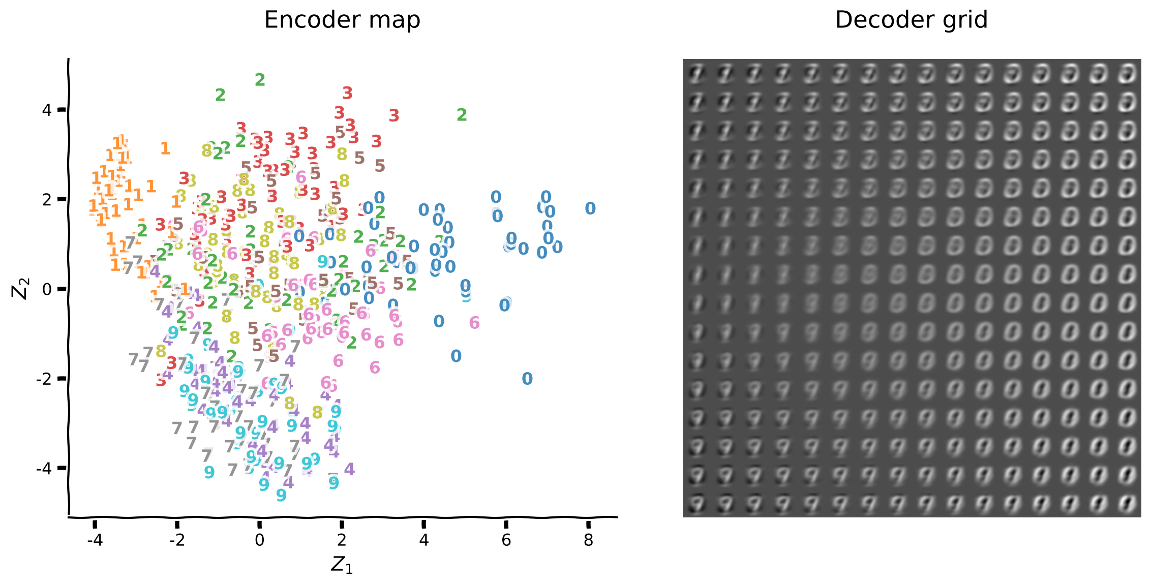
プロット関数plot_latent_generativeは、高次元の入力を2次元潜在空間にエンコードし、元の次元にデコードする様子を可視化します。この関数は2つのプロットを生成します：

エンコーダーマップは入力画像から潜在空間座標 $(z_1, z_2)$ へのマッピングを示し、数字ラベルを重ねて表示します
デコーダーグリッドは潜在空間座標 $(z_1, z_2)$ のグリッドからの再構成画像を示します

潜在空間の可視化 $

潜在空間表現は新しい座標系 $(z_1, z_2)$ であり、高次元データの重要な構造を捉えていることが期待されます。各入力の座標は他の入力の座標との相対関係が重要であり、数字のクラス間の分離性に注目することが多いです。

エンコーダーマップは潜在空間の構造を直接理解する手助けとなります。潜在空間は座標 $(z_1, z_2)$ のみを含み、数字ラベルなどの追加情報を重ねて潜在空間の構造を洞察します。

左のプロットは数字ラベルなしの生の潜在空間表現で、右のプロットは数字ラベルを重ねたものです。

生の潜在空間の可視化 $

セクション 3.1: PCAによるMNISTの潜在空間

コーディング演習 1: PCA潜在空間の可視化（2次元）

チュートリアルW1D5 次元削減ではPCA分解を紹介しました。主成分2つ（PCA1とPCA2）の場合、2次元の潜在空間が生成されます。

PCA潜在空間の可視化 $

チュートリアルW1D5では、PCA分解を直接実装したほか、パッケージscikit-learnのモジュールsklearn.decompositionを使っても実装しました。このモジュールには次元削減技術として有用な複数の行列分解アルゴリズムが含まれています。

使い方は非常に簡単で、以下は切断特異値分解（Truncated SVD）の例です：

svd = decomposition.TruncatedSVD(n_components=2)

svd.fit(input_train)

svd_latent_train = svd.transform(input_train)
svd_latent_test = svd.transform(input_test)

svd_reconstruction_train = svd.inverse_transform(svd_latent_train)
svd_reconstruction_test = svd.inverse_transform(svd_latent_test)

この演習ではdecomposition.PCA（ドキュメントはこちら）を使ってPCA分解を行います。

指示:

decomposition.PCAを2次元で初期化する
.fitメソッドでinput_trainに適合させる
input_testの潜在空間表現を取得する
plot_latent_generativeで潜在空間を可視化する

ヘルパー関数: plot_latent_generative

この関数を確認するため、以下の行のコメントを外してください。

# @title

# @markdown Execute this cell to inspect `plot_latent_generative`!
help(plot_latent_generative)

####################################################
## TODO for students: perform PCA and visualize latent space and reconstruction
raise NotImplementedError("Complete the make_design_matrix function")
#####################################################################
# create the model
pca = decomposition.PCA(...)
# fit the model on training data
pca.fit(...)
# transformation on 2D space
pca_latent_test = pca.transform(...)

plot_latent_generative(pca_latent_test, y_test, pca.inverse_transform,
                       image_shape=image_shape)

解答例はこちら$

出力例:

# @title Submit your feedback
content_review(f"{feedback_prefix}_Visualize_PCA_latent_space_Exercise")

セクション 3.2: PCAの定性的解析

エンコーダーマップはエンコーダーが数字クラスをどれだけうまく区別しているかを示します。数字1と0は第一主成分軸の反対側に位置し、同様に数字9と3は第二主成分軸の反対側に位置しています。

デコーダーグリッドは潜在空間座標から画像をどれだけうまく復元できているかを示します。全体的に数字1、0、9が最も認識しやすいです。

これらの観察をよりよく理解するために主成分を調べましょう。主成分はpca.components_として利用可能で、以下に示します。

主成分

第一主成分は数字0を正の値（白色）で、数字1を負の値（黒色）で符号化しています。カラーマップは最小値を黒、最大値を白で表し、数字0と1の第一主成分軸の座標を見ることで符号がわかります。

第一主成分軸は数字の「太さ」を符号化しています：左側が細い数字、右側が太い数字です。

同様に第二主成分は数字9を正の値（白色）、数字3を負の値（黒色）で符号化しています。

第二主成分軸は「太さ」以外の別の側面を符号化しています（なぜでしょうか？）。

再構成グリッドは数字4と7が数字9と区別しにくく、数字2と3も同様であることを示しています。

指示:

以下のセルを実行してください
再構成サンプルを何度かプロットして、数字の混同の様子を視覚的に把握しましょう（ベクトル化画像の可視化にはキーワードimage_shapeを使います）。

pca_components = pca.components_

plot_row(pca_components, image_shape=image_shape)

pca_output_test = pca.inverse_transform(pca_latent_test)

plot_row([input_test, pca_output_test], image_shape=image_shape)

セクション4: ANNオートエンコーダー

単一の隠れ層を持つ浅いANNオートエンコーダーを実装してみましょう。

単一隠れ層のANNオートエンコーダー

ANNオートエンコーダーの設計（32次元）

ここでは、研究プロジェクトの初期探索段階に最適なPyTorchモデルを素早く構築するための手法を紹介します。

チュートリアルW3D4で紹介したオブジェクト指向プログラミング（OOP）は、モデルのアーキテクチャや構成要素をより深く理解した後に最適な選択肢となります。

この簡潔な手法を使うと、W3D4チュートリアル1のDeepNetReLUと同等のネットワークを以下のように定義できます。

model = nn.Sequential(nn.Linear(n_input, n_hidden),
                      nn.ReLU(),
                      nn.Linear(n_hidden, n_output))

効率的なニューラルネットワークの設計と訓練には、隠れ層の数、損失関数、最適化関数、ミニバッチサイズなどの選択肢の中から適切なものを選ぶための考慮、経験、試行が必要です。これらのハイパーパラメータの選択は、これらのシステムと学習ダイナミクスに対する分析的理解が深まるにつれて、より工学的なプロセスになっていくでしょう。

以下の参考文献は、ニューラルネットワークの設計やベストプラクティスを学ぶのに最適です：

Michael NielsenによるNeural Networks and Deep Learningは初心者に最適な参考書です
Ian Goodfellow、Yoshua Bengio、Aaron CourvilleによるDeep Learningは詳細かつ広範な内容を提供します
L. SmithによるA disciplined approach to neural network hyper-parameters: Part 1 -- learning rate, batch size, momentum, and weight decayはハイパーパラメータ設定の効率的な方法を解説しています

コーディング演習2: ANNオートエンコーダーの設計

ボトルネック層にはencoding_dim=32のReLU（整流関数）ユニットを使い、出力層にはシグモイドユニットを使います。活性化関数についてはこちら $、整流関数については[こちら](https://$ en.wikipedia.org/wiki/Rectifier_(neural_networks))$をご覧ください。

ReLUユニット

単一隠れ層のANNオートエンコーダー

出力層のシグモイドユニットと互換性を持たせるために、画像の値を0から1の範囲に再スケーリングしました（なぜかは考えてみてください）。このようなマッピングは一般性を損なうものではなく、任意の（有限の）範囲は0から1の範囲に一対一対応で写像できます。

ReLUとシグモイドの両方のユニットはエンコーダーとデコーダーに非線形計算を提供します。シグモイドユニットはさらに、出力値が入力と同じ範囲に収まることを保証します。これらのユニットはReLUに置き換えることもできますが、その場合は出力値が時々負の値や1を超える値になることがあります。デコーダーのシグモイドユニットは、データに関するドメイン知識を数値的制約として表現しています。

指示

nn.Sequentialは層のサイズ(input_shape, encoding_dim, input_shape)でANNを定義・初期化します
nn.Linearは入力と出力のサイズを引数に線形層を定義します
nn.ReLUとnn.SigmoidはそれぞれReLUとシグモイドユニットを表します
plot_rowを使って入力画像と出力画像の初期出力を可視化しましょう

encoding_size = 32

######################################################################
## TODO for students: add linear and sigmoid layers
raise NotImplementedError("Complete the make_design_matrix function")
#####################################################################
model = nn.Sequential(
    nn.Linear(input_size, encoding_size),
    nn.ReLU(),
    # insert your code here to add the layer
    # nn.Linear(...),
    # insert the activation function
    # ....
    )

print(f'Model structure \n\n {model}')

サンプル出力

Sequential(
  (0): Linear(in_features=784, out_features=32, bias=True)
  (1): ReLU()
  (2): Linear(in_features=32, out_features=784, bias=True)
  (3): Sigmoid()
)

解答を見る$

# @title Submit your feedback
content_review(f"{feedback_prefix}_Design_ANN_autoencoder_Exercise")

with torch.no_grad():
  output_test = model(input_test)

plot_row([input_test.float(), output_test], image_shape=image_shape)

オートエンコーダーの訓練（32次元）

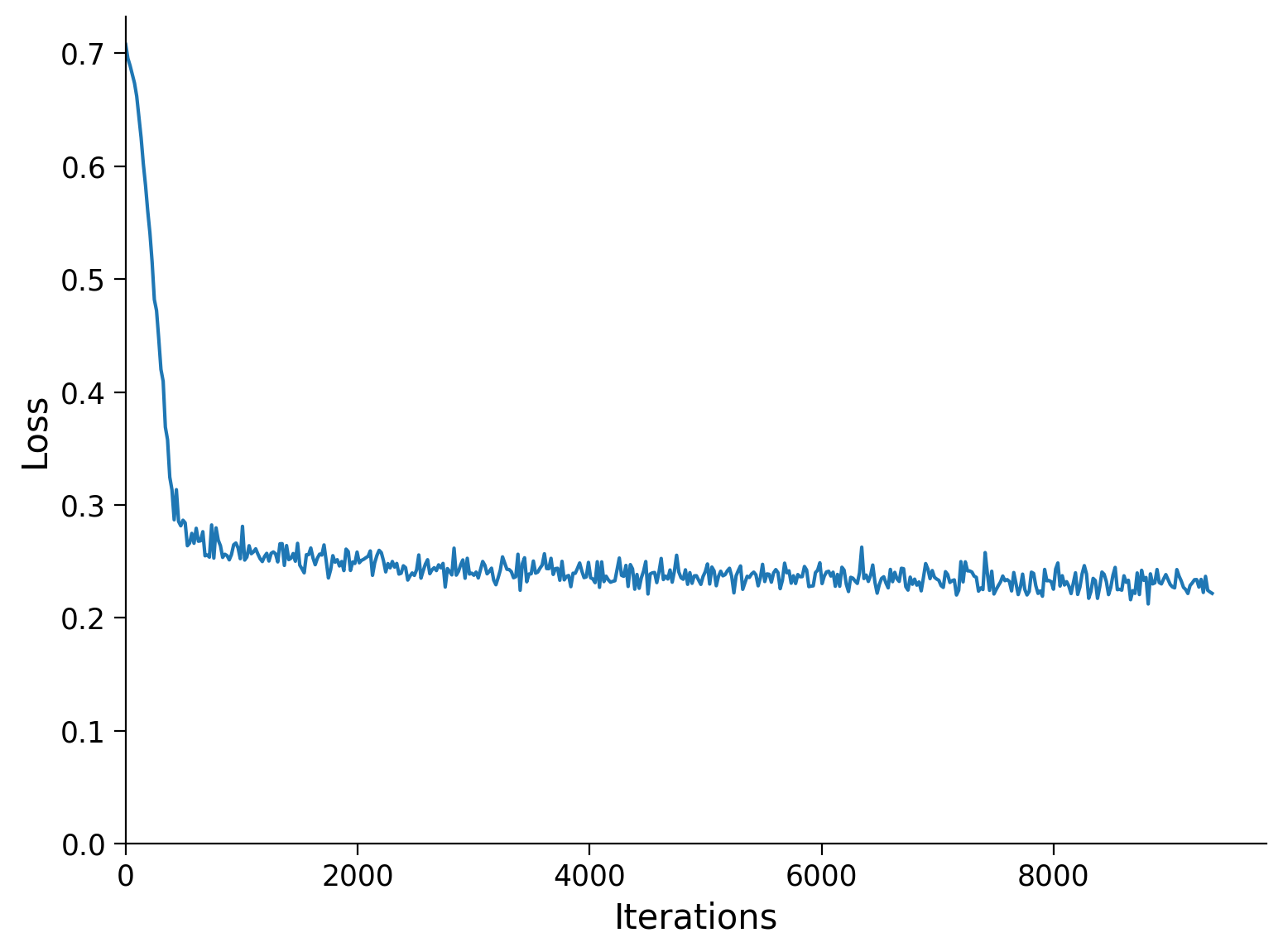
runSGD関数はAdamオプティマイザ（optim.Adam）を用いた確率的勾配降下法でオートエンコーダーを訓練し、平均二乗誤差（MSE、nn.MSELoss）と二値交差エントロピー（BCE、nn.BCELoss）のいずれかを選択できます。

以下の図は損失関数のイメージで、 $\hat{Y}$ は出力値、 $Y$ はターゲット値を表します。

MSE損失

BCE損失

n_epochs=10エポック、batch_size=64でrunSGDを使いMSE損失でネットワークを訓練し、いくつかの再構成サンプルを可視化しましょう。

以下のセルを実行してモデルの構築と訓練を行ってください！

encoding_size = 32

model = nn.Sequential(
    nn.Linear(input_size, encoding_size),
    nn.ReLU(),
    nn.Linear(encoding_size, input_size),
    nn.Sigmoid()
    )

n_epochs = 10
batch_size = 64

runSGD(model, input_train, input_test, criterion='mse',
       n_epochs=n_epochs, batch_size=batch_size)

with torch.no_grad():
  output_test = model(input_test)

plot_row([input_test[test_selected_idx], output_test[test_selected_idx]],
         image_shape=image_shape)

損失関数の選択

損失関数は訓練中にネットワークが最適化する対象を決定し、これは再構成画像の視覚的な特徴に反映されます。

例えば、白い領域の中央に孤立した黒いピクセルは非常にありそうにないノイズのように見えます。ネットワークは白いピクセルが黒くなったりその逆のシナリオを最大限に罰することで、そうした状況を避けることを優先できます。

以下の図は、ターゲットピクセル値 $Y=1$ 、出力が $\hat{Y}\in [0, 1]$ の範囲にある場合のMSEとBCEの比較です。MSE損失はこの範囲で穏やかな二次関数的増加を示します。BCE損失は暗いピクセル（ $\hat{Y}$ が0.4未満）で急激に増加することに注目してください。

BCEとMSE損失の比較

より客観的に比較するために、それらの導関数 $d\,\text{Loss}/d\,\hat{Y}$ を見てみましょう。MSE損失の導関数は傾き $-2$ の線形ですが、BCEは暗いピクセル値で $1/\hat{Y}$ のように急増します（なぜか考えてみてください）。

BCEとMSE損失の導関数比較

両損失関数のy軸スケールを揃えるために、プロット範囲を $[0.05, 1]$ に制限しています（なぜか考えてみてください）。

BCE損失に切り替えて、白いピクセルが黒くなった場合やその逆を最大限に罰する効果を確認しましょう。ネットワークは両方の損失でよく収束するため、視覚的な違いは微妙です。

MSE損失での再構成画像に孤立した白/黒ピクセル領域がないか探してください。

まずMSE損失で2エポック訓練し、次にBCE損失で同様に訓練して違いを強調します。

以下のセルを実行して、それぞれMSEとBCEで訓練してください。

encoding_size = 32
n_epochs = 2
batch_size = 64

model = nn.Sequential(
    nn.Linear(input_size, encoding_size),
    nn.ReLU(),
    nn.Linear(encoding_size, input_size),
    nn.Sigmoid()
    )

runSGD(model, input_train, input_test, criterion='mse',
       n_epochs=n_epochs, batch_size=batch_size, verbose=True)

with torch.no_grad():
  output_test = model(input_test)

plot_row([input_test[test_selected_idx], output_test[test_selected_idx]],
         image_shape=image_shape)

encoding_size = 32
n_epochs = 2
batch_size = 64

model = nn.Sequential(
    nn.Linear(input_size, encoding_size),
    nn.ReLU(),
    nn.Linear(encoding_size, input_size),
    nn.Sigmoid()
    )

runSGD(model, input_train, input_test, criterion='bce',
       n_epochs=n_epochs, batch_size=batch_size, verbose=True)

with torch.no_grad():
  output_test = model(input_test)

plot_row([input_test[test_selected_idx], output_test[test_selected_idx]],
         image_shape=image_shape)

ANNオートエンコーダーの設計（2次元）

ボトルネックユニット数をencoding_size=2に減らすと、PCAと同様に2次元の潜在空間が生成されます。エンコーダーマップの座標 $(z_1, z_2)$ はボトルネック層のユニット活性化を表します。

オートエンコーダーのエンコーダーマップ $

encoderコンポーネントは潜在空間の $(z_1, z_2)$ 座標を提供し、decoderコンポーネントは $(z_1, z_2)$ から画像の再構成を生成します。オートエンコーダーネットワークの層のシーケンスを指定することで、これらのサブネットワークを定義できます。

model = nn.Sequential(...)
encoder = model[:n]
decoder = model[n:]

このアーキテクチャは32ユニットのボトルネック層ではうまく機能しますが、2ユニットでは収束に失敗します。ボーナスセクションの演習でこの失敗の原因と対処法（重みの初期化改善や活性化関数の変更）を理解しましょう。

ここではボトルネック層にPreLUユニットを採用し、負の活性化に学習可能なパラメータを加えています。この変更により、ボトルネック層が2ユニットでもデータをモデル化する余地が増えます。

PreLUユニット

指示

以下のセルを実行してください

encoding_size = 2

model = nn.Sequential(
    nn.Linear(input_size, encoding_size),
    nn.PReLU(),
    nn.Linear(encoding_size, input_size),
    nn.Sigmoid()
    )

encoder = model[:2]
decoder = model[2:]

print(f'Autoencoder \n\n {model}')

print(f'Encoder \n\n {encoder}')

print(f'Decoder \n\n {decoder}')

オートエンコーダーの訓練（2次元）

n_epochs=10エポック、batch_size=64でrunSGDとBCE損失を使ってネットワークを訓練し、潜在空間を可視化しましょう。

以下のセルを実行してオートエンコーダーを訓練してください！

n_epochs = 10
batch_size = 64

# train the autoencoder
runSGD(model, input_train, input_test, criterion='bce',
       n_epochs=n_epochs, batch_size=batch_size)

with torch.no_grad():
  latent_test = encoder(input_test)

plot_latent_generative(latent_test, y_test, decoder,
                       image_shape=image_shape)

2次元における表現力

2次元ボトルネックを持つ浅いオートエンコーダーの潜在空間表現はPCAに似ています。線形次元削減手法が非線形オートエンコーダーと比較可能なのはなぜでしょうか？

線形活性化関数を用いMSE損失でオートエンコーダーを訓練することはPCAを行うことに非常に似ています。区分的線形ユニット、シグモイド出力ユニット、BCE損失を使っても、この挙動は質的に変わらないようです。ネットワークは学習可能なパラメータの容量が不足しており、非線形演算を活かしてデータの非線形性を捉えることができていません。

デコーダーマップを並べてプロットすると、表現の類似性が明らかです。うまくクラスタリングされている数字のクラスと、まだ混ざっているクラスを探してみましょう。

以下のセルを実行してPCAとオートエンコーダー（2次元）の比較を行いましょう！

plot_latent_ab(pca_latent_test, latent_test, y_test,
               title_a='PCA', title_b='Autoencoder (2D)')

まとめ

このチュートリアルでは、低次元表現の作成と可視化の基本技術に慣れ、浅いオートエンコーダーの構築を学びました。

PCAと浅いオートエンコーダーは、非線形性を持つオートエンコーダーにもかかわらず、2次元潜在空間で類似した表現力を持つことがわかりました。

浅いオートエンコーダーは、エンコード・デコードにおける非線形演算を活かし、データの非線形パターンを捉えるための十分な学習可能パラメータを持っていません。

次のチュートリアルでは、MNIST認知課題に取り組むために必要なより豊かな内部表現を学習するために、オートエンコーダーのアーキテクチャを拡張します。

# @title Video 3: Wrap-up
from ipywidgets import widgets
from IPython.display import YouTubeVideo
from IPython.display import IFrame
from IPython.display import display


class PlayVideo(IFrame):
  def __init__(self, id, source, page=1, width=400, height=300, **kwargs):
    self.id = id
    if source == 'Bilibili':
      src = f'https://player.bilibili.com/player.html?bvid={id}&page={page}'
    elif source == 'Osf':
      src = f'https://mfr.ca-1.osf.io/render?url=https://osf.io/download/{id}/?direct%26mode=render'
    super(PlayVideo, self).__init__(src, width, height, **kwargs)


def display_videos(video_ids, W=400, H=300, fs=1):
  tab_contents = []
  for i, video_id in enumerate(video_ids):
    out = widgets.Output()
    with out:
      if video_ids[i][0] == 'Youtube':
        video = YouTubeVideo(id=video_ids[i][1], width=W,
                             height=H, fs=fs, rel=0)
        print(f'Video available at https://youtube.com/watch?v={video.id}')
      else:
        video = PlayVideo(id=video_ids[i][1], source=video_ids[i][0], width=W,
                          height=H, fs=fs, autoplay=False)
        if video_ids[i][0] == 'Bilibili':
          print(f'Video available at https://www.bilibili.com/video/{video.id}')
        elif video_ids[i][0] == 'Osf':
          print(f'Video available at https://osf.io/{video.id}')
      display(video)
    tab_contents.append(out)
  return tab_contents


video_ids = [('Youtube', 'V0gVrkyFd0Y'), ('Bilibili', 'BV1Eh411Z7TB')]
tab_contents = display_videos(video_ids, W=854, H=480)
tabs = widgets.Tab()
tabs.children = tab_contents
for i in range(len(tab_contents)):
  tabs.set_title(i, video_ids[i][0])
display(tabs)

# @title Submit your feedback
content_review(f"{feedback_prefix}_WrapUp_Video")

ボーナス

2次元ReLUユニットでの失敗モード

ボトルネック層に2ユニット、ReLUユニット、デフォルトの重み初期化を用いたアーキテクチャは、ミニバッチの順序やオプティマイザの選択などにより収束に失敗することがあります。この失敗モードを示すために、まず乱数生成器（RNG）を設定して失敗例を再現します：

torch.manual_seed(0)
np.random.seed(0)

続いて、成功例を再現するためにRNGを設定します：

torch.manual_seed(1)

n_epochs=10エポック、batch_size=64でネットワークを訓練し、それぞれの場合のエンコーダーマップと再構成グリッドを確認してください。

次に、エンコーダーとデコーダーの重みの分布を調べます。エンコーダーは入力ピクセルをボトルネックユニットにマッピングし（エンコーダー重みの形状は(2, 784)）、デコーダーはボトルネックユニットを出力ピクセルにマッピングします（デコーダー重みの形状は(784, 2)）。

ネットワークモデルは通常、0に近いランダムな重みで初期化されます。PyTorchの線形層のデフォルトの重み初期化は、入力ユニット数fan_inに基づき、[-limit, limit]の一様分布からサンプリングされ、 $limit=1/\sqrt{fan_in}$ です。

初期化時の重み分布と訓練後の分布を比較します。訓練中に学習されなかった重みは初期分布のままですが、SGDで調整された重みは分布が変化します。

エンコーダーの重みはベル型の分布になることもあります。これはSGDが各初期重みに正負の増分を加えるためで、中心極限定理（CLT）により独立した増分ならガウス分布になるはずですが、非ガウス性はSGD増分の相互依存性の指標となります。

指示:

以下のセルを実行してください
失敗例としてtorch.manual_seed = 0から始める
エンコーダーマッピングが単一軸に収束していることを確認する
収束しなかった次元が変化していない重みに対応していることを確認する
成功例としてtorch.manual_seed = 1に変更する
学習可能パラメータ（重みとバイアス）を取得する方法は $help(get_layer_weights)$ を参照する

encoding_size = 2
n_epochs = 10
batch_size = 64

# set PyTorch RNG seed
torch_seed = 0

# reset RNG for weight initialization
torch.manual_seed(torch_seed)
np.random.seed(0)

model = nn.Sequential(
    nn.Linear(input_size, encoding_size),
    nn.ReLU(),
    nn.Linear(encoding_size, input_size),
    nn.Sigmoid()
    )

encoder = model[:2]
decoder = model[2:]

# retrieve weights and biases from the encoder before training
encoder_w_init, encoder_b_init = get_layer_weights(encoder[0])
decoder_w_init, decoder_b_init = get_layer_weights(decoder[0])

# reset RNG for minibatch sequence
torch.manual_seed(torch_seed)
np.random.seed(0)

# train the autoencoder
runSGD(model, input_train, input_test, criterion='bce',
       n_epochs=n_epochs, batch_size=batch_size)

# retrieve weights and biases from the encoder after training
encoder_w_train, encoder_b_train = get_layer_weights(encoder[0])
decoder_w_train, decoder_b_train = get_layer_weights(decoder[0])

with torch.no_grad():
  latent_test = encoder(input_test)
  output_test = model(input_test)

plot_latent_generative(latent_test, y_test, decoder, image_shape=image_shape)

plot_row([input_test[test_selected_idx], output_test[test_selected_idx]],
         image_shape=image_shape)

plot_weights_ab(encoder_w_init, encoder_w_train, decoder_w_init,
                decoder_w_train)

ボーナスコーディング演習3: 重み初期化の選択

ReLUユニットの失敗モードを回避する改善された重み初期化として、Kaiming uniformがよく使われます。これは重みテンソルの入力ユニット数 $f\_in$ に基づき、一様分布 $\mathcal{U}(-limit, limit)$ からサンプリングし、 $limit=\sqrt{6/fan\_in}$ とします（詳細はこちらの論文$を参照）。オートエンコーダーの全重みをKaiming uniformでリセットする例：

model.apply(init_weights_kaiming_uniform)

もう一つの方法は、平均0、標準偏差 $1/\sqrt{fan\_in}$ の正規分布 $\mathcal{N}(\mu, \sigma^2)$ からサンプリングするものです。オートエンコーダーの最後の2層を除く全層をKaiming normalでリセットする例：

model[:-2].apply(init_weights_kaiming_normal)

重み初期化について詳しく知りたい場合、以下の参考文献が良い出発点です：

指示:

init_weights_kaiming_uniformでエンコーダーの重みをリセットする
init_weights_kaiming_normalでリセットした場合と比較する
詳細は $help(init_weights_kaiming_uniform)$ と $help(init_weights_kaiming_normal)$ を参照する

encoding_size = 2
n_epochs = 10
batch_size = 64

# set PyTorch RNG seed
torch_seed = 0

model = nn.Sequential(
    nn.Linear(input_size, encoding_size),
    nn.ReLU(),
    nn.Linear(encoding_size, input_size),
    nn.Sigmoid()
    )

encoder = model[:2]
decoder = model[2:]

# reset RNGs for weight initialization
torch.manual_seed(torch_seed)
np.random.seed(0)

######################################################################
## TODO for students: reset encoder weights and biases
raise NotImplementedError("Complete the code below")
#####################################################################
# reset encoder weights and biases
encoder.apply(...)

# retrieve weights and biases from the encoder before training
encoder_w_init, encoder_b_init = get_layer_weights(encoder[0])
decoder_w_init, decoder_b_init = get_layer_weights(decoder[0])

# reset RNGs for minibatch sequence
torch.manual_seed(torch_seed)
np.random.seed(0)

# train the autoencoder
runSGD(model, input_train, input_test, criterion='bce',
       n_epochs=n_epochs, batch_size=batch_size)

# retrieve weights and biases from the encoder after training
encoder_w_train, encoder_b_train = get_layer_weights(encoder[0])
decoder_w_train, decoder_b_train = get_layer_weights(decoder[0])

解答を見る$

出力例:

# @title Submit your feedback
content_review(f"{feedback_prefix}_Choosing_weight_initialization_Bonus_Exercise")

with torch.no_grad():
  latent_test = encoder(input_test)
  output_test = model(input_test)

plot_latent_generative(latent_test, y_test, decoder,
                       image_shape=image_shape)

plot_row([input_test[test_selected_idx], output_test[test_selected_idx]],
         image_shape=image_shape)

plot_weights_ab(encoder_w_init, encoder_w_train, decoder_w_init,
                decoder_w_train)

活性化関数の選択

特定の重み初期化の代わりに、この文脈でより良い性能を示す活性化ユニットを選択する方法もあります。ここではボトルネック層にPreLUユニットを使い、負の活性化に学習可能なパラメータを加えます。

この変更により、ReLUユニットよりもオートエンコーダーがデータをモデル化するための余地が少し増えます。

PreLUユニット

指示:

以下のセルを実行してください

encoding_size = 2
n_epochs = 10
batch_size = 64

# set PyTorch RNG seed
torch_seed = 0

# reset RNGs for weight initialization
torch.manual_seed(torch_seed)
np.random.seed(0)

model = nn.Sequential(
    nn.Linear(input_size, encoding_size),
    nn.PReLU(),
    nn.Linear(encoding_size, input_size),
    nn.Sigmoid()
    )

encoder = model[:2]
decoder = model[2:]

# retrieve weights and biases from the encoder before training
encoder_w_init, encoder_b_init = get_layer_weights(encoder[0])
decoder_w_init, decoder_b_init = get_layer_weights(decoder[0])

# reset RNGs for minibatch sequence
torch.manual_seed(torch_seed)
np.random.seed(0)

# train the autoencoder
runSGD(model, input_train, input_test, criterion='bce',
       n_epochs=n_epochs, batch_size=batch_size)

# retrieve weights and biases from the encoder after training
encoder_w_train, encoder_b_train = get_layer_weights(encoder[0])
decoder_w_train, decoder_b_train = get_layer_weights(decoder[0])

with torch.no_grad():
  latent_test = encoder(input_test)

plot_latent_generative(latent_test, y_test, decoder, image_shape=image_shape)

plot_weights_ab(encoder_w_init, encoder_w_train, decoder_w_init,
                decoder_w_train)

NMFの定性的解析

sk.decomposition.NMF（ドキュメントはこちら）を使って*非負値行列因子分解（NMF）*を行います。

正の行列 $W$ と $H$ の積がデータ行列 $X$ を近似します。すなわち、 $X \approx W H$ です。

$W$ の列はPCAの主成分と同じ役割を果たします。

数字クラスの0と1は潜在空間で最も離れており、より良くクラスタリングされています。

第1成分を見ると、画像が徐々に数字クラス0に似ていく様子がわかります。第2成分は数字クラス1と9の混合で、同様の進行を示しています。

データは0付近の失敗モードを避けるために0.5だけシフトされています。これはスケーリングの選択に関連していると思われます。シフトなしでも試してみてください。

パラメータinit='random'は初期の非負ランダム行列のスケールを調整し、より良い結果をもたらすことが多いので、こちらも試してみてください。

以下のセルを実行してNMFを実行しましょう。

nmf = decomposition.NMF(n_components=2, init='random')

nmf.fit(input_train + 0.5)

nmf_latent_test = nmf.transform(input_test + 0.5)

plot_latent_generative(nmf_latent_test, y_test, nmf.inverse_transform,
                       image_shape=image_shape)

nmf_components = nmf.components_

plot_row(nmf_components, image_shape=image_shape)

nmf_output_test = nmf.inverse_transform(nmf_latent_test)

plot_row([input_test, nmf_output_test], image_shape=image_shape)